Numerical Investigation of Flow through a Valve during Charge Intake in a DISI -Engine Using Large Eddy Simulation

Abstract

Apart from electric vehicles, most internal combustion (IC) engines are powered while burning petroleum-based fossil or alternative fuels after mixing with inducted air. Thereby the operations of mixing and combustion evolve in a turbulent flow environment created during the intake phase and then intensified by the piston motion and influenced by the shape of combustion chamber. In particular, the swirl and turbulence levels existing immediately before and during combustion affect the evolution of these processes and determine engine performance, noise and pollutant emissions. Both the turbulence characteristics and the bulk flow pattern in the cylinder are strongly affected by the inlet port and valve design. In the present paper, large eddy simulation (LES) is appraised and applied to studying the turbulent fluid flow around the intake valve of a single cylinder IC-engine as represented by the so called magnetic resonance velocimetry (MRV) flow bench configuration with a relatively large Reynolds number of 45,000. To avoid an intense mesh refinement near the wall, various subgrid scale models for LES; namely the Smagorinsky, wall adapting local eddy (WALE) model, SIGMA, and dynamic one equation models, are employed in combination with an appropriate wall function. For comparison purposes, the standard RANS (Reynolds-averaged Navier–Stokes) k-$\epsilon$ model is also used. In terms of a global mean error index for the velocity results obtained from all the models, at first it turns out that all the subgrid models show similar predictive capability except the Smagorinsky model, while the standard k-$\epsilon$ model experiences a higher normalized mean absolute error (nMAE) of velocity once compared with MRV data. Secondly, based on the cost-accuracy criteria, the WALE model is used with a fine mesh of ≈39 millions control volumes, the averaged velocity results showed excellent agreement between LES and MRV measurements, revealing the high prediction capability of the suggested LES tool for valve flows. Thirdly, the turbulent flow across the valve curtain clearly featured a back flow resulting in a high speed intake jet in the middle. Comprehensive LES data are generated to carry out statistical analysis in terms of (1) evolution of the turbulent morphology across the valve passage relying on the flow anisotropy map, (2) integral turbulent scales along the intake-charge stream, (3) turbulent flow properties such as turbulent kinetic energy, turbulent velocity and its intensity within the most critical zone in intake-port and along the port length, it further transpires that the most turbulence are generated across the valve passage and these are responsible for the in-cylinder turbulence.

1. Introduction

In the IC-engine design, port/valve and cylinder head contour play crucial roles as they are largely responsible for the overall flow structure inside an engine cylinder. During the intake, a very large shear layer is induced along the high speed intake jet. The shape, orientation and location of intake valve together with the design of the cylinder head determine the in-cylinder global structure, known as tumble or swirl motion [1,2,3,4]. These global structures further cascade into smaller ones and it influences—in the case of gasoline direct injection spark ignition (DISI) engine—the air-fuel mixing and subsequent flow pattern inside the combustion chamber. Affected by the cyclic piston motion, the inherent variability of the flow field plays a critical role in determining the engine control parameters to achieve optimum performance and fuel economy especially in the direct-injection spark-ignition (DISI) engine [1,5]. Such a behavior is more pronounced in stratified-charge operation, since the performance as a whole is highly influenced by the flow field variability along with the local mixing and distribution of air-fuel-residual within the piston-bowl. This is known to affect the propagation of the spark-kernel and the flame, thus may be responsible for the engine mis-fire in the worst case scenario [6,7,8,9].

It is thus obvious that all physical process in the IC-engine are cross-correlated to each other and it is often difficult to cover all in a single test set-up. The latter allows us to rather gain a detailed understanding of only the individual process phenomenon. Focused on the intake valve flow, it is worth mentioning that the intake stroke is characterized by very high speed jets through a constricted valve passage. These jets often generate shear-flow along the near-stagnant cylinder volume resulting in early flow turbulence which is further sustained by transient piston/valve motion and shape/contour of piston-bowl/cylinder-head [10,11].

The performance of intake valve/port is mostly investigated in steady-state flow configurations [2,12,13] with fixed lift position for the valves. However, the applicability of such results to transient engine behavior is always subjected to questions. However, recent works by Freudenhammer et al. [14,15], which compared such measurement data with transient results from realistic DISI-engine operations [16], highlight the ability of such measurements to characterize the flow through valve curtain along with the global flow structures. The adopted measurement technique also allows us to capture a 3-dimensional in-cylinder mean flow field making it useful for detailed validation of numerical simulations.

In the context of numerical analysis, Reynolds Averaged Navier Stokes (RANS) simulation is well established in supporting engineering design, development and optimization tasks for over last decades. It provides ensemble averaged flow properties reasonably good in quick time as it can run properly for relatively coarse mesh [6,7,17]. However, with the RANS approach, it is difficult to resolve the cyclic variability of in-cylinder flow dynamics also known as cycle-to-cycle variations (CCV) [18,19,20,21,22,23,24]. This cyclic variability is the prime source of the unregulated combustion, especially in the context of knocking, misfire, pollutant and $N{O}_x$ emission [20,21,22,23,24,25]. Applying direct numerical simulations (DNS), all the scales can be fully resolved, and cycle-to-cycle variations of in-cylinder flow dynamics addressed very well. DNS of IC-engine configurations are very rare owing to associated high computational cost, which increases exponentially with the engine speed and compression ratio [19]. However, DNS was indeed carried out, albeit for an engine-like geometry featuring an axis-symmetric piston-cylinder assembly, only for a non-fired case with a single valve [19]. DNS for IC-engines under realistic conditions have not yet been reported. In contrast to RANS and DNS, large eddy simulation (LES) offers a trade-off between the computational cost and scale resolving capabilities. LES requires intermediate cost of computation, as it allows to capture fully the large scale flow structures, while the small scales are modeled using sub-grid scale (SGS) stress closure methodology [26,27], which can be applied to modern combustion systems [28,29]. Further, LES has been successful in resolving the cycle-to-cycle variations of in-cylinder flow-fields and subsequently assessing its influence on the mixing, combustion and pollutant emission as reported by many researchers [20,21,22,23,24]. Nevertheless, it should be noted that, due to complex real engine configuration carrying out LES for many engine cycles with moving piston/valves even for a non-fired case requires considerable numerical effort especially to control mesh resolution and quality with moving or adaptive mesh methodology. A more detailed review is provided in References [25,30].

In order to carry out in-depth studies of individual processes, it is very useful to isolate and reduce the complexity of the engine configuration. In this regard, the present study focuses on the steady-state flow configuration with two main objectives: (1) to evaluate the influence of intake valve/port especially in the generation of early flow turbulence and the development of global structures (tumble or swirl motions) which have a strong impact on the in-cylinder flow and on the subsequent processes, and (2) to assess the predictive capability of the adopted numerical methodology [13,31,32] in view of future work towards a reliable analysis of in-cylinder flow including moving intake and exhaust valves under fully realistic operating conditions. The present computational studies mostly rely on the available 3D measurement data gained from the so-called MRV flow-bench configuration [14], which represents a single-cylinder direct-injection spark-ignition engine [16].

The present paper is organized as follows. In Section 2, the adopted LES methodology is introduced. In Section 3 the MRV configuration is briefly described, and the numerical set up outlined. In Section 4, the obtained results are presented and discussed. First, the LES methodology is evaluated comprehensively by comparing simulation results with MRV experimental data in terms of first statistical moments. Then, a methodology is provided to gain further insight into the transient phenomena while carrying out turbulence statistical analysis in the critical zone along the intake jet. Section 5 summarizes the essential findings of this work.

2. LES Methodology

A classical LES methodology in its incompressible formulation along with various subgrid scale (SGS) models are used and integrated into the open source software OpenFOAM [33]. In this respect, the filtered governing equations of mass and momentum are solved as they are given by:

$$\frac{\partial {\overline{U}}_i}{\partial x_i}=0$$

(1)

$$\frac{\partial {\overline{U}}_i}{\partial t}+\frac{\partial }{\partial x_j}\left({\overline{U}}_i{\overline{U}}_j\right)=\frac{\partial \overline{p}}{\partial x_i}+\frac{\partial }{\partial x_i}\left(\nu \left(\frac{\partial {\overline{U}}_i}{\partial x_j}+\frac{\partial {\overline{U}}_j}{\partial x_i}\right)\right)-\frac{\partial {\tau }_{ij}^{sgs}}{\partial x_i},$$

(2)

where $\overline{U}$ and $\overline{p}$ are the filtered or resolved velocity and pressure fields, respectively. ${\tau }_{ij}^{sgs}$ represents the SGS stress tensor. It is modeled by a linear eddy-viscosity approach based on Boussinesq hypothesis as

$${\tau }_{ij}^{sgs}=\frac{2}{3}{k}^{sgs}{\delta }_{ij}-{\nu }^{sgs}\left(\frac{\partial {\overline{U}}_i}{\partial x_j}+\frac{\partial {\overline{U}}_j}{\partial x_i}\right).$$

(3)

In the present work, the isotropic part of the sub-grid stress tensor is included in a modified filtered pressure term defined as

$$\overline{P}=\overline{p}+\frac{2}{3}{k}^{sgs}.$$

(4)

The SGS viscosity, ${\nu }^{sgs}$, can be closed by using diverse SGS or turbulence models [34]. In the present work, it is postulated as

$${\nu }^{sgs}={\left(C_m{\Delta }_g\right)}^2{\mathsf{\Theta }}_m$$

(5)

where $C_m$ is a model coefficient, ${\displaystyle {\Delta }_g={\left({\Delta }_x{\Delta }_y{\Delta }_z\right)}^{1/3}}$, and ${\displaystyle {\mathsf{\Theta }}_m}$ an operator specific to the SGS models utilized, namely the Smagorinsky, WALE, SIGMA, one-equation model. They are listed in

Table 1. Operator ${\mathsf{\Theta }}_m$ and model coefficient $C_m$ for various LES models applied. ${\overline{D}}_{ij}$ is the filtered strain rate tensor, $k^{sgs}$ the subsgrid-scale kinetic energy, ${\overline{S}}_{ij}^d$ the traceless symmetric part of the squared velocity gradient and ${\sigma }_1,{\sigma }_2,{\sigma }_1$ are the three singular values of the velocity gradient.

LES Models	Operator ${\mathsf{\Theta }}_{\mathit{m}}$	Model Coefficient ${\mathit{C}}_{\mathit{m}}$
Smagorinsky	${\displaystyle \sqrt{2{\overline{D}}_{ij}{\overline{D}}_{ij}}}$	${\displaystyle C_s}$ = 0.18
WALE	${\displaystyle \frac{{\left({\overline{S}}_{ij}^d{\overline{S}}_{ij}^d\right)}^{2/3}}{{\left({\overline{D}}_{ij}{\overline{D}}_{ij}\right)}^{5/2}+{\left({\overline{S}}_{ij}^d{\overline{S}}_{ij}^d\right)}^{5/4}}}$	${\displaystyle C_W}$ = 0.5
SIGMA	$\frac{{\displaystyle {\sigma }_3\left({\sigma }_1-{\sigma }_2\right)\left({\sigma }_2-{\sigma }_3\right)}}{{\sigma }_1^2}$	${\displaystyle C_{\sigma }}$ = 1.5
one-equation	$\frac{{\displaystyle \sqrt{k_{sgs}}}}{C_m{\Delta }_g}$	${\displaystyle C_k}$ = 0.18, ${\displaystyle C_e}$ = 1

.

In particular, the WALE model has been systematically verified and tested for wall bounded flows. It is proven to correctly capture the asymptotic behavior of velocity near the wall [34] while requiring optimal computational costs/accuracy in comparison to the standard Smagorinsky model with Van Driest wall damping function, SIGMA and dynamic-one-equation models. All these models are used to compare their prediction capability of the influence of the intake valve/port, especially in the generation of early flow turbulence and the development of global structures (tumble or swirl motions). For this purpose, a global mean error index experienced by each SGS model will be examined.

Since with a relatively high Reynolds number, which is the case in the present work, the wall adapted LES will be computationally intensive as the size of the wall mesh is very small (14 $\mathsf{\mu }$m) for corresponding “$y^{+}\le 1.0$”, a Spalding wall function is applied to the viscosity term at the wall boundary [35] to overcome this issue. Based on the universal equilibrium stress model, this wall function is applicable for the present $y^{+}$ value at the wall and defined as:

$$y^{+}=u^{+}+\frac{1}{E}\left(e^{k{u}^{+}}-1-k{u}^{+}-{\left(k{u}^{+}\right)}^2-\frac{1}{2}{\left(k{u}^{+}\right)}^3\right)$$

(6)

where $y^{+}=y{u}_{\tau }/\nu$ and $u^{+}=u/u_{\tau }$, respectively, while constants $E=9.1$ and $k=0.41$. With the known value of the $y_p$ and $u_p$ at the wall, Equation (6) can be solved iteratively to obtain the shear velocity $u_{\tau }$ at the wall. Thereby, the subgrid viscosity at the first cell at the wall can be calculated as:

$${\nu }_{sgs}=\frac{y_p{u}_{\tau }^2}{u_p}-\nu$$

(7)

where $\nu$ is the molecular viscosity and $y_p$ the distance of the first grid cell from the wall with a cell point velocity of $u_p$. As mentioned above, all the modeled filtered equations have been integrated into the OpenFOAM code [33] for which a detailed description of the numerical features of the model implementation can be found in Ries et al. [34].

3. Engine Configuration and Numerical Setup

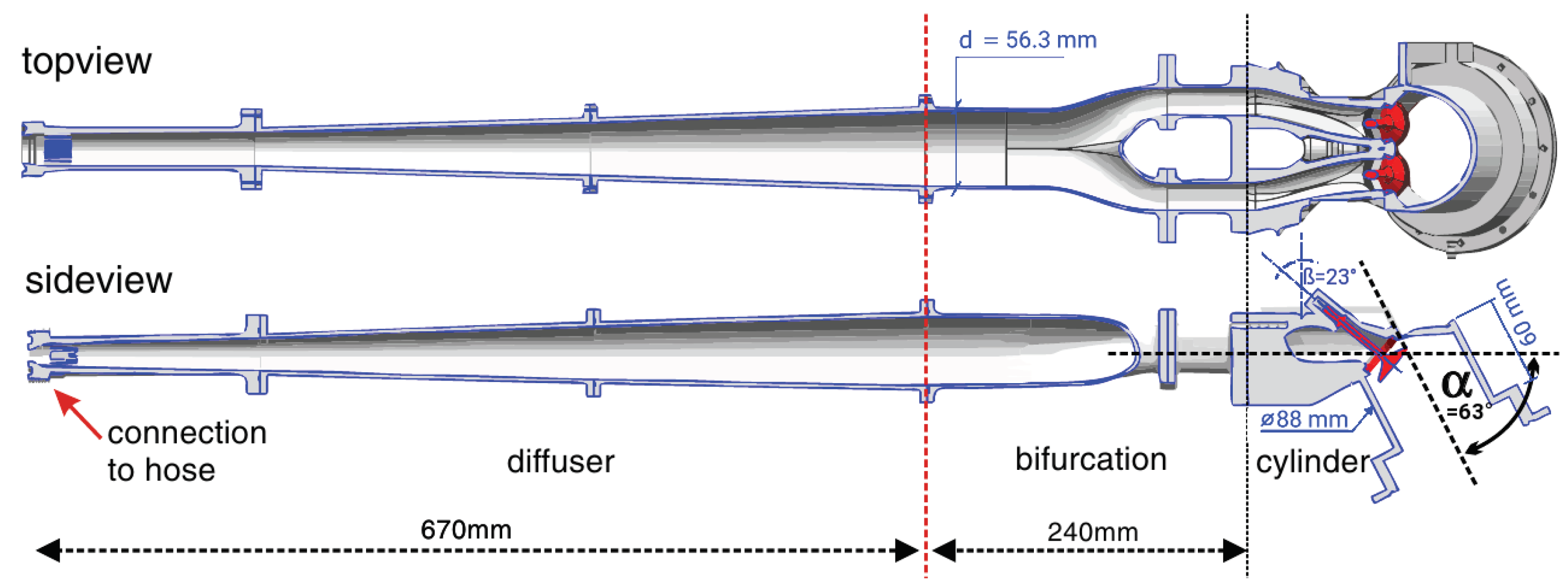
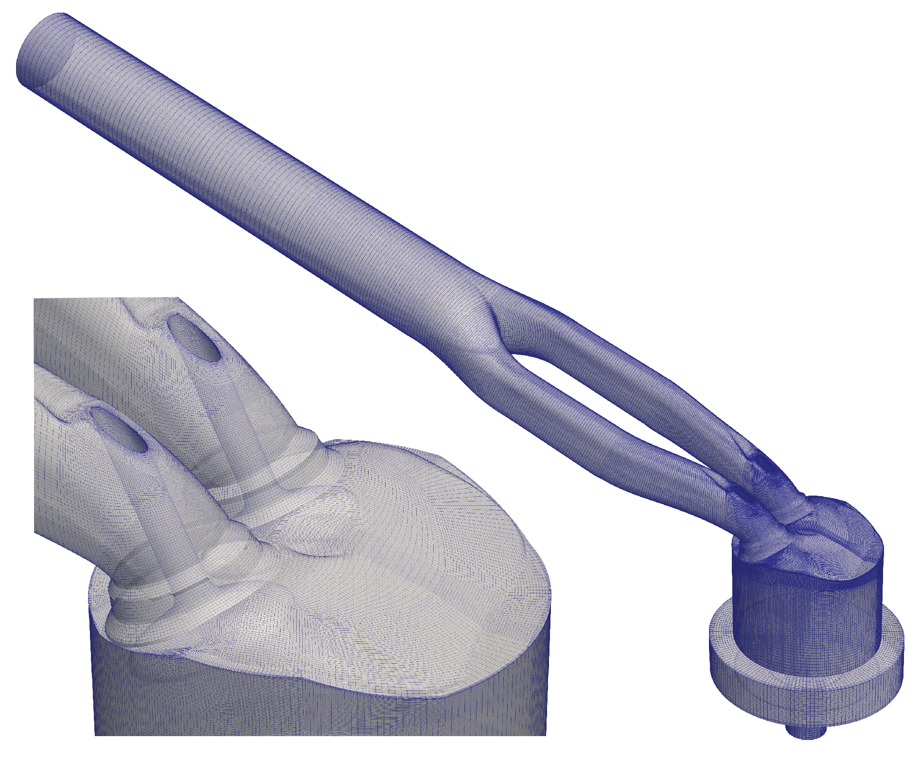
3.1. Engine Configuration

The engine configuration under investigation represents a single-cylinder direct-injection spark-ignition (DISI) optical engine [16]. It features a twin-cam, overhead-valve pent-proof cylinder head with dual-port intake system to provide a tumble flow motion within the combustion chamber. Both bore and stroke of this engine are 86 mm with geometric compression ratio of 8.5. This engine is used to carry out MRV measurement by Freudenhammer et al. [14] into 1:1 scale produced from Polyamide by laser-sintering (EOS, Formiga P100). The sectional (top and side) views of the MRV model with diffuser and bifurcation is shown in Figure 1. The working fluid enters into diffuser with a total length of 670 mm with end-to-end diametric expansion from 25.4 mm to 56.3 mm. The remaining part of the geometry represents an actual wall-guided engine configuration [16] corresponding to an engine status of 270${}^{\circ }$bTDC with an intake valve lift of 9.21 mm. De-ionized water is used as a working fluid with the possibility of increasing the water temperature by heating coils. This way, the operating Reynolds number can be achieved by lowering water viscosity by heating.

In the present case, the water temperature is kept at 50 ${}^{\circ }$C with volumetric flow rate of 66 L/min which corresponds to a bulk Reynolds number of approx. 45,000 which is close to the range of real engine operating conditions. More details about the MRV measurement techniques and relevant post-processing method are provided in [15]. It should be noted that, in the present work, the diffuser part is not included, instead the port is extruded four diameter (4d) of intake port beyond red dotted line in Figure 1. This is represented numerically by the computational domain as shown in Figure 2.

3.2. Numerical Setup: Inlet and Initial Conditions

To carry out reliable CFD simulations, it is very important to provide appropriate initial and inlet conditions based on the flow configurations (transient and steady state). In the case of the RANS approach, it is often possible to describe turbulence properties in terms of the more readily known parameters such as turbulence intensity, turbulent viscosity ratio, and turbulence length scale. With these parameters in hand it is possible to calculate the appropriate inlet boundary values for RANS turbulence models. However, in case of LES, which is inherently transient, the initial and boundary conditions play a vital role. The initial conditions largely influence the averaging time and total run time for statistically independent results. Improper turbulence at inlet can affect the whole results especially the overall variance of the flow field along with the cycle-to-cycle variations obtained from LES.

In the present work, the issue with initial condition is dealt in two steps. At first the LES is carried out for coarse mesh for sufficient long simulation. Secondly, the flow field is interpolated into the finer mesh in order to reduce the computational time by minimizing the total run time for statistically independent results. Various methods for the in-flow boundary for LES have been suggested (e.g., References [36,37]). Klein et al. [36] proposed a so called digital based generation of in-flow field by generating artificial velocity data which reproduces first and second order one point statistics as well as a locally given auto-correlation function which was further developed by Kempf et al. [37] to apply for arbitrary geometrical configurations. Considering the fact that the MRV flow-bench represents a steady-state volumetric flow of water for relatively longer duration, in the present approach, the in-flow condition is generated in two major steps. First, a fully developed turbulent pipe flow is simulated. Secondly this flow field is mapped into extruded intake port. The fully turbulent field is then achieved by setting periodic boundary condition along the extruded port length and simulating for sufficiently long physical time to achieve statistical independent flow field. In case of incompressible solver, it is imperative to prescribe initial turbulent field. This is accomplished by generating isotropic turbulence in equidistant mesh, then interpolating the fluctuating field into the pipe before superposing the velocity based on power-law profile corresponding to bulk flow [38]. This velocity field has to be solved only in the extended port with periodic boundary condition for a sufficiently long duration to achieve statistically steady state. The resultant flow field is then interpolated into MRV flow-bench configuration applying the so called recycling method of boundary condition along the same section of pipe to retain the turbulence field in the pipe and inlet region as suggested by Lund et al. [39]. In this way, one avoids the complicated process of storing the field data of extended port for each time-step and then imposing into the inlet of MRV flow-bench for successive time-steps.

3.3. Numerical Setup: Prior Evaluation of Simulation Measures

Before carrying out the LES study, it is very important to assess how long (physical time) the simulation has to be performed in order to achieve statistically independent results for both mean flow velocity and variance. In the case of simple pipe or channel flow, it is possible to roughly guess the simulation time. In the present case, it is advantageous to make good use of the basic features of the RANS model, which offers a preliminary evaluation of turbulent time and length scales. It should be noted that, depending upon the complexity of the configuration, these scales can vary in many orders of magnitude. Therefore, the total simulation time should be chosen judiciously based on the criticality of region and location to be compared with the available experimental finding. In fact, this evaluation also provides proper guidelines to the experimentalists how long the sample data should be collected for the same reason of statistical independency. In a plane across one of the intake valves where experimental data will be compared against LES later on, Figure 3 shows the evaluated turbulent time and length scales obtained by using the standard k-$\epsilon$ model [40] based simulation. It is clearly visible from the results that the time and length scales are very small immediately downstream to the valves, while they are sufficiently large further left downstream and into the cylinder chamber. This is the location where the large tumble structure is formed. This indicates that less physical time is required to achieve flow-field with acceptable stochastic error close to the valve as compared to the rest of the domain. Therefore, the assessed simulation time of 10 s is sufficient for the LES analysis for the present flow bench as suggested in a recent work by Ries et al. [34]. Therefore, in the present work fully hex-hedral mesh is used to discretize the complete domain. Thus LES is first performed for mesh (≈4.9 millions) using WALE model with wall function for physical time of 10 s. Instead of initializing simulations from scratch for the fine-mesh (≈39 millions CVs), the final flow field of coarse mesh at 10 s is therefore linearly mapped into fine mesh and allowed to develop the flow-field for further 4 s, including the last 3 s to achieve the averaged flow field. Similar procedure is followed to initialize the flow-field for other SGS models for LES (SIGMA, Smagorinsky, dynamic-one-equation), however simulations are here carried only with coarse mesh (≈4.9 millions).

4. Results and Discussion

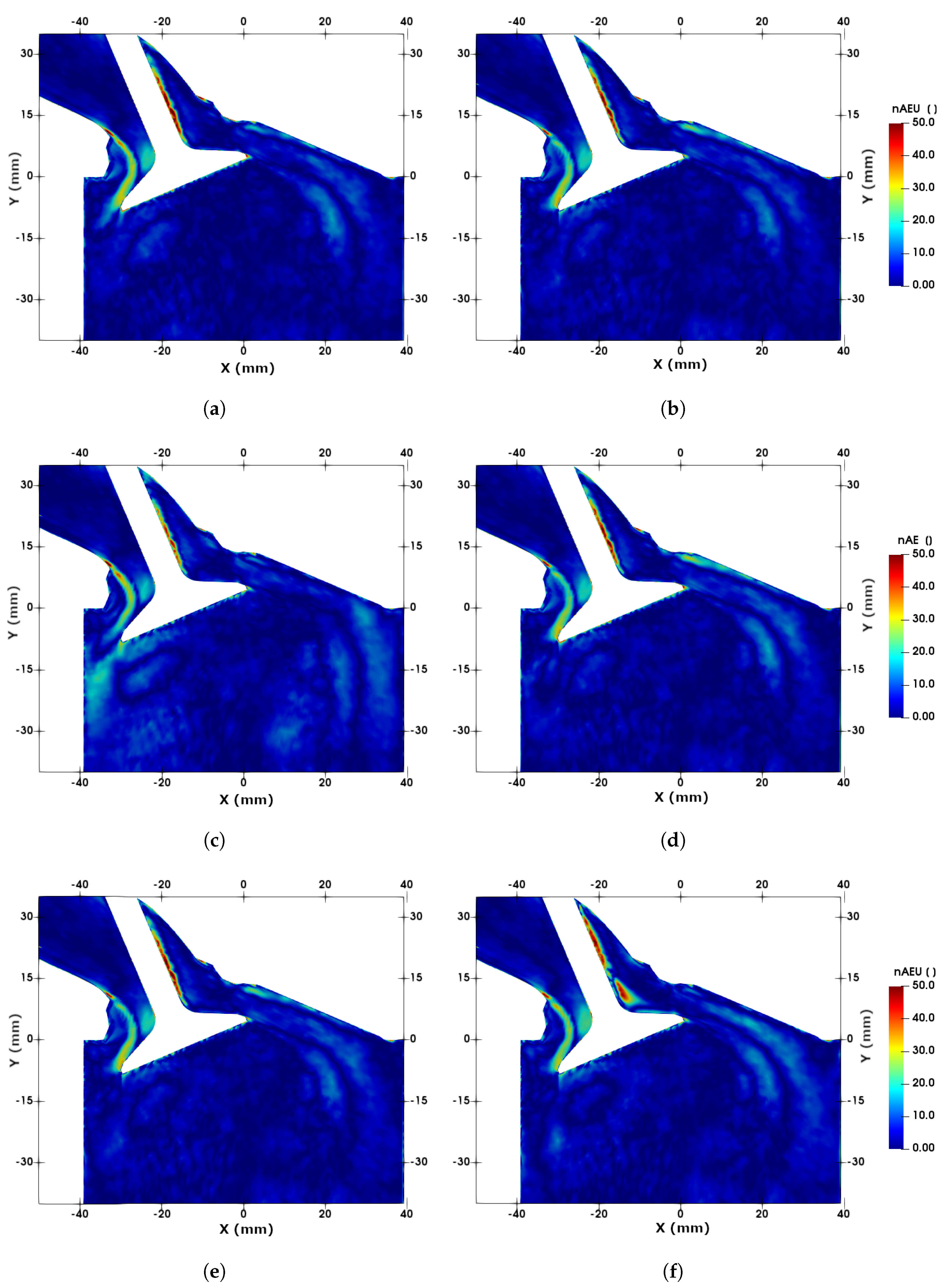
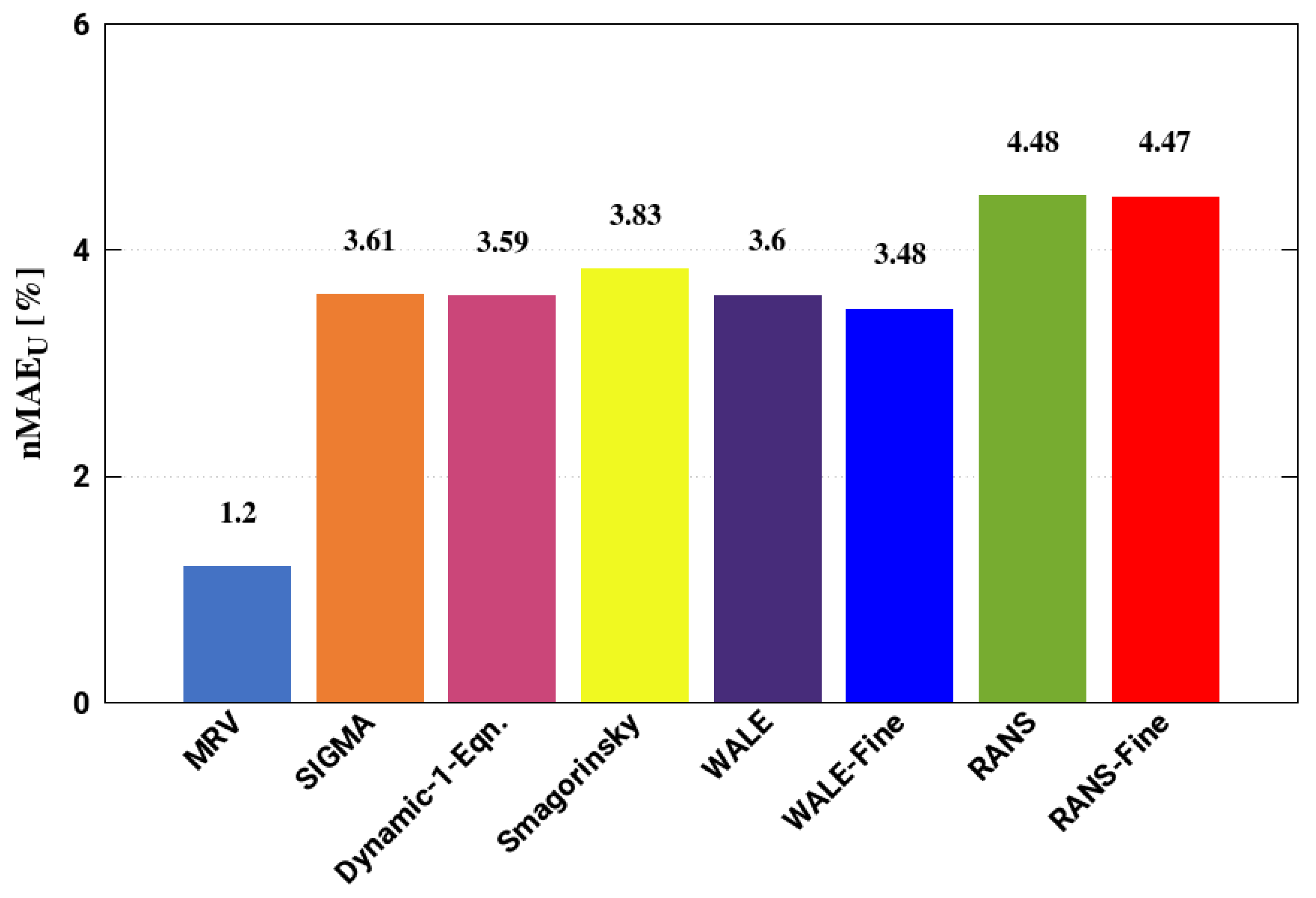
4.1. Evaluation of SGS/Turbulence Models Based on Error Analysis

At first, based on the error index also know as normalized absolute error (nAE), the adopted turbulence models are evaluated for charge intake and in-cylinder flow dynamics in DISI engine. This error index for variable $\psi$ is defined as [34,41];

$${\mathrm{nAE}}_{{\psi }_i}=100\left[\frac{|{\psi }_i^{sim}-{\psi }_i^{ref}|}{d\left({\psi }^{ref}\right)}\right]$$

(8)

where i is the spatial location, the superscripts ‘$ref$’ and ‘$sim$’ represent the reference data and simulated data, respectively. The MRV measurement data for velocity is taken as reference data in the present case, with $d(.)$ representing the difference between the maximal and minimal value of the reference data ${\psi }^{ref}$. The obtained nAE are compared for each turbulence model cases along one of the valve plane as shown in Figure 4. At first, nAE profile are compared for fine and coarse mesh by using the WALE model (see Figure 4a,b). The comparison shows almost identical distribution of error index throughout the plane in both cases with relatively higher value along shear layer in the left side of the valve and the right side of the valve stem. The latter can be attributed to the non-physical MRV velocity profile along the valve stem wall. Since identical distributions of nAE are obtained for both coarse and fine grids, it is obvious for computational cost reasons to use only the coarse mesh in order to compare the nAE as experienced by other turbulence models (namely; standard RANS k-$\epsilon$, SGS dynamic-one- equation, SIGMA and Smagorinsky models) as displayed in Figure 4c–f.

It turns out that these models reveal a similar trend as for the WALE model with the exception of the RANS model in Figure 4c. The discrepancy of the error distribution for the standard k-$\epsilon$ visibly higher downstream of the left side of valve can be attributed to the inability of RANS model to resolve the highly transient charge intake flow.

To further quantitatively compare these models, a global mean error metric “lnMAE-normalized mean absolute error)” is introduced by summing up the nAE in Equation (8) for the whole domain or spatial locations n [34,41];

$${\mathrm{nMAE}}_{\psi }=100\left[\frac{\frac{1}{n}{\sum }_{i=1}^n|{\psi }_i^{ref}-{\psi }_i^{sim}|}{d\left({\psi }^{ref}\right)}\right]$$

(9)

Figure 5 depicts a comparison of nMAE provided once the applied turbulence/SGS models are involved. All the SGS models lead to a similar prediction accuracy as the nMAE achieved in of the same order of magnitude. In particular, the WALE, SIGMA and the dynamic one-equation models are relatively more accurate than Smagorinsky model. This suggests that the error contribution due to SGS modeling is comparatively small to the other sources of error (e.g., reference data, boundary conditions, averaring time, numerical methods, near wall modeling etc.). However, considering the computational cost, the WALE model emerges as most favorable one [34]. Therefore, it will be used for further investigation analysis throughout the paper. As expected for RANS model, the nMAE is higher while the error is still within the engineering limit of 5%. This suggests that RANS model can still be used for initial stage of engineering analysis.

4.2. Validation: Comparisons of LES Results with MRV Data

In order to appraise the LES results, both qualitative and quantitative comparisons are carried out against MRV data using only the WALE model, now under a fine mesh environment.

Figure 6 displays a comparison of the velocity contour obtained from MRV measurement and LES results in a tumble plane cutting across one of the intake valve. The results demonstrate qualitative good agreement where the LES capture well the tumble motion structure inside the engine-cylinder with two vortex clearly visible both sides of the valve. The maximum velocity is observed mostly in the valve passage caused by a reduced cross-sectional flow area due to the presence of valve. The regular flow structure inside the intake-port is disturbed by the valve-stem resulting in a vortex similar to Karman-vortex-shedding, which is ultimately responsible of turbulence initiation and its further generation. Affected by the valve shape and its orientation together with the cylinder head contour, the flow is guided through to the engine cylinder volume resulting in a tumble motion. In the left side of the valve, a back flow can also be observed both in MRV and LES. This flow further compresses the intake-flow stream and the velocity gets further increased towards the right hand side. Such back flow is also responsible for reduction of the overall trapped air-mass inside the engine cylinder once the intake-valve is closed.

Figure 7 shows a comparison of the velocity contour in the cross-tumble plane. The maximum velocity can be seen above the intake valve. The flow is further redirected through the valve periphery into the cylinder volume similar to an annular flow. The intake stream on the other side of valve strikes the cylinder wall and straightens downwards. At the region between the valves, jets from both sides impinge on each other and further evolve in a similar way. This ultimately leads to the formation of vortex-flow in cross-tumble plane as it can be seen in Figure 7 for both MRV and LES results. Figure 8 depicts a comparison of velocity contour in a plane below the valves ($Y=-10$). The annular flow over the valve periphery is quite visible in this view. Due to canted intake-valves the flow is directed more towards the right hand side. The higher velocity due to constricted flow cross-sectional area can be seen at valve edges near the cylinder wall. The reduced velocity behind the valve (left side) is mainly due to the wake formation as visible in Figure 8. The overall flow structure looks symmetric across the line $Z=0$ for both MRV and LES results representing good qualitative agreements. The intake jet is further compared with MRV data by plotting the radial velocity along the valve curtain in Figure 9. The evidence of back flow (with -ve velocity) is clearly visible both in the MRV measurement and LES results. Such back flow influences the in-cylinder flow dynamic by a two-fold effect: first it reduces the total entrapped mass inside the engine cylinder when valve is closed, secondly it also pushes the flow towards the centre of valve curtain as the higher velocity can be seen at the center of valve curtain (see Figure 9). The latter phenomena is mostly responsible for generating tumble motion and its strength.

Furthermore, the quantitative comparison of the velocity from MRV measurement and LES is depicted in Figure 10 in the middle section ($(Z=0$ mm)) of the engine cylinder at various Y-locations. At the location close to the cylinder head $(Y=-9$ mm) the velocity magnitude is higher especially towards the intake valve, while this magnitude diminishes further downwards eventually generating a velocity peak towards the right side due to intake charge stream. The velocity profile is further compared across one of the intake port in Figure 11. Close to the valve $(Y=-9$ mm) a distinct velocity peak is clearly visible in both sides of the valve which is predominant towards the left side owing to a reduced passage. Further downstream these peaks get flattened. Similar profile can be observed across another valve in Figure 12, however with a slight difference owing to the non-symmetric cylinder head. The assessed qualitative and quantitative LES results evidence the capability of the WALE model in predicting the DISI in-cylinder flow dynamics.

4.3. Turbulence and Statistical Analysis in the Engine Cylinder Chamber and the Intake Port

During the intake stroke, the air enters the combustion chamber through the intake port with high velocity. Thus, high kinetic energy of the fluid flow during intake stroke results subsequently in high turbulence of the in-cylinder fluid flow. Since the in-cylinder turbulent flow is known as a leading parameter which determines the performance and the efficiency of IC-engines, the identification of the aerodynamic phenomena which take place at the level of the valves is an important step for the comprehension of physical processes which evolve in IC-engines.

To isolate such phenomena, detailed flow information is required. However, the MRV measurement technique allows mostly for capturing mean flow only; the transient nature of in-cylinder flow dynamics cannot be resolved experimentally, and associated quantities be made available. Therefore, comprehensive LES data are used to provide a detailed insight about the state of turbulence properties inside the cylinder chamber. In addition to the velocity fields in Figure 10, Figure 11 and Figure 12, the turbulent kinetic energy is plotted in Figure 13 and Figure 14 for planes in the cylinder mid-section and cutting across one of intake valve, respectively. It appears clearly that a higher turbulent kinetic energy is visible immediately downstream to the valves. Especially in Figure 13a, along the middle section of cylinder chamber, the higher turbulent kinetic energy can be attributed to two intake jets (from both valves) which impinge on each other as seen also in Figure 7. Further downstream, more homogeneous and gradually decreasing profile for the turbulent kinetic energy is observed in Figure 13b,c. However, along the plane cutting across a valve, a peak in turbulent kinetic energy arises in the left side (see Figure 14a) due to a high flow re-circulation as obvious in Figure 6. Afterwards, the turbulent intensity gradually decreases further downstream in the cylinder chamber (see Figure 14b,c).

Considering both the locations in the intake port and in the cylinder, the anisotropy of the flow is extracted and plotted in the so called invariant map in Figure 15 according to Lumley and Newman [42]. At first, Figure 15a depicts the anisotropy map on a cross-sectional plane in the intake duct showing a fully developed pipe flow scenario in which the three-components isotropic turbulence exists for the pipe core region, while two components state prevails near the wall due to the damping of wall normal components. This result corresponds to the classical anisotropy map of turbulent pipe flow. The state of turbulence and its morphology are further examined along the intake-charge-stream in both sides of the valve as illustrated in Figure 15b. Thereby, it is visible that the generation of turbulence through the intake valve is nearly isotropic in nature.

Next, a statistical analysis is carried out in terms of integral time scales, turbulent kinetic energy, and turbulence intensity. For that purpose the magnitude velocity samples are extracted at five locations (see Figure 16a) for each time steps while maintaining the constant LES time-step with maximum CFL $<0.75$ and mean CFL $<0.012$. These time-series data are used to calculate the integral time scale which can be linked to the degree of turbulence. The integral time in these locations are increasing down stream (see Figure 16b). This behavior can be attributed to the decreasing characteristic velocity due to the turbulent flow dispersion downstream. Numerically, this also implies the need for simulations for a longer physical time in order to achieve well averaged mean and variance of the flow-field with same stochastic error at further upstream.

4.4. Turbulence Evolution along the Intake Port

As pointed out above, it is a well established fact that the flow through the ports/valves is one of the key factors influencing the global flow structure and subsequent turbulence properties inside the engine cylinder chamber. In order to gain more insight into the turbulence properties through the intake port and then to determine the most critical zone along the port length, cross-sectional LES results are extracted at equidistant location along the whole port length in stream-wise direction. Some of these cross-sections are highlighted in Figure 17a for representation purpose. Figure 17b–d depict the evolution of turbulent kinetic energy, turbulence velocity and intensity, respectively along the port length. It is quite evident that the most of the turbulence are generated when the flow is passing through the valve passage as the turbulent kinetic energy and fluctuating velocity are higher close the port valves. The turbulence intensity is nearly constant $(\approx$7%) for most of the pipe length where the cross-sectional area is representing the standard turbulence level for pipe flow. The first noticeable increase in turbulence intensity is observed at the location where the port is bifurcated into two streams. This can be attributed to the decreased mean flow velocity due to higher cross-sectional area while turbulence level remains constant (see the turbulent kinetic energy and velocity plot). The intensity is then observed to increase gradually owing to higher turbulent kinetic energy along the smaller cross-sectional port length. The intensity is relatively higher at the valve passage owing to very high turbulent kinetic energy in this region.

In order to analyze the distribution of turbulence properties across the cross-section, the variances of turbulent kinetic energy and its intensity are plotted as shown in Figure 18. The variance of the turbulent kinetic energy is very low for the initial uniform cross-sectional length of the intake port showing relatively a well developed and homogeneous flow turbulence, while at later part of the length especially across the intake valve flow it is highly non-homogeneous. This trend is also similar in case of the turbulent intensity, however with high degree of non-homogeneity even for the region of the initial pipe length.

In order to further analyze the turbulent phenomena when the intake jets leave the valve passage and enters into the cylinder volume, the turbulence properties calculated from LES are plotted in Figure 19 across the valve curtain. The turbulent kinetic energy (see Figure 19b) can be seen higher around the periphery of main intake jet induced by large shear layer due to sharp velocity gradient. Corresponding turbulent fluctuating velocity is depicted in Figure 19c showing similar trend. The turbulence intensity is plotted in Figure 19d. It shows mostly homogeneous and lower values only in the region of high intake jet where the mean velocity is actually high, while it is high and non-homogeneous in the region of back flow and lower mean velocity (see Figure 19a).

5. Summary

In this paper, LES was applied to investigate the turbulent fluid flow around the intake valve of a single cylinder IC-engine represented by so called MRV (magnetic resonance velocimetry) flow bench configuration for which 3-dimensional MRV experimental data are available. Thereby various turbulence/SGS models have been employed to close the filtered momentum equation. Instead of resolving the wall fully, the well-known Spalding wall function was applied to avoid intense mesh refinement near the wall in combination of diverse SGS models, namely the Smagorinsky, wall adapting local eddy (WALE) model, SIGMA, dynamic one equation models. The standard RANS k-$\epsilon$ model was involved for comparison purposes. From this study, the following inferences could be drawn:

• the WALE model featured relatively a less normalized absolute error relying on the velocity field and emerged as the suitable choice among all the models applied. The standard RANS k-$\epsilon$ model has proven to be less accurate.
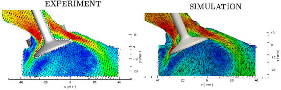
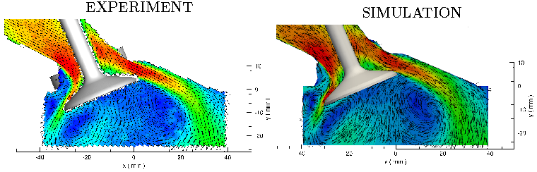
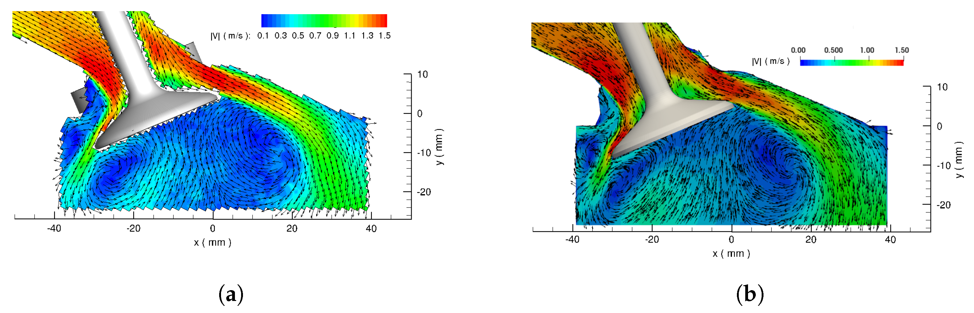
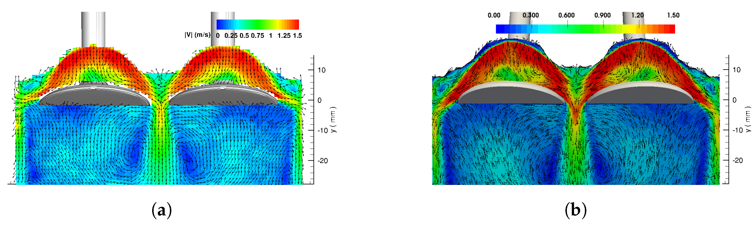
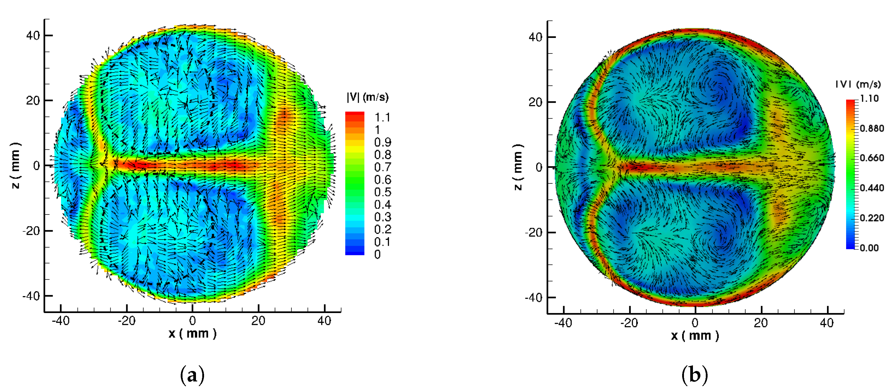
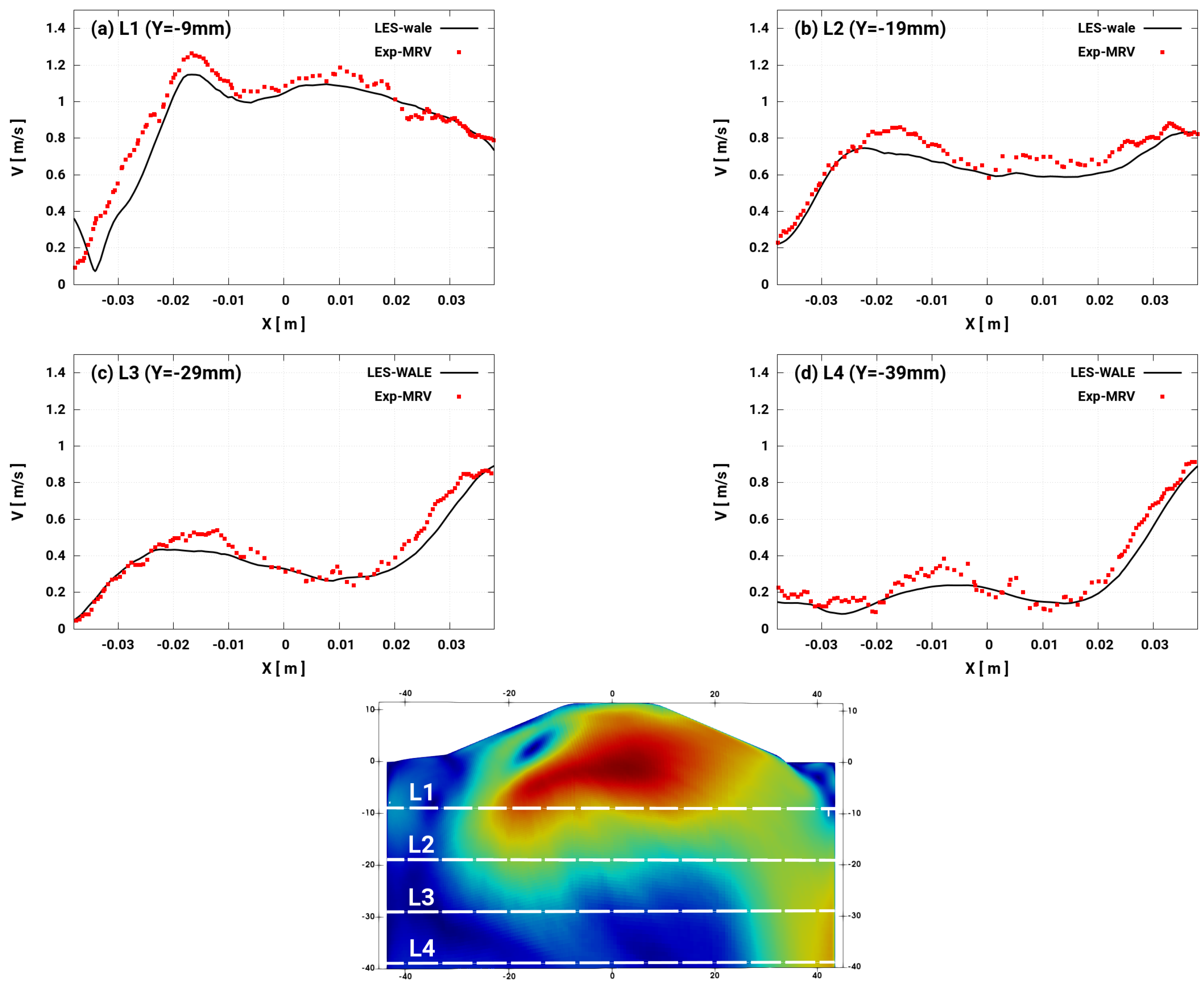
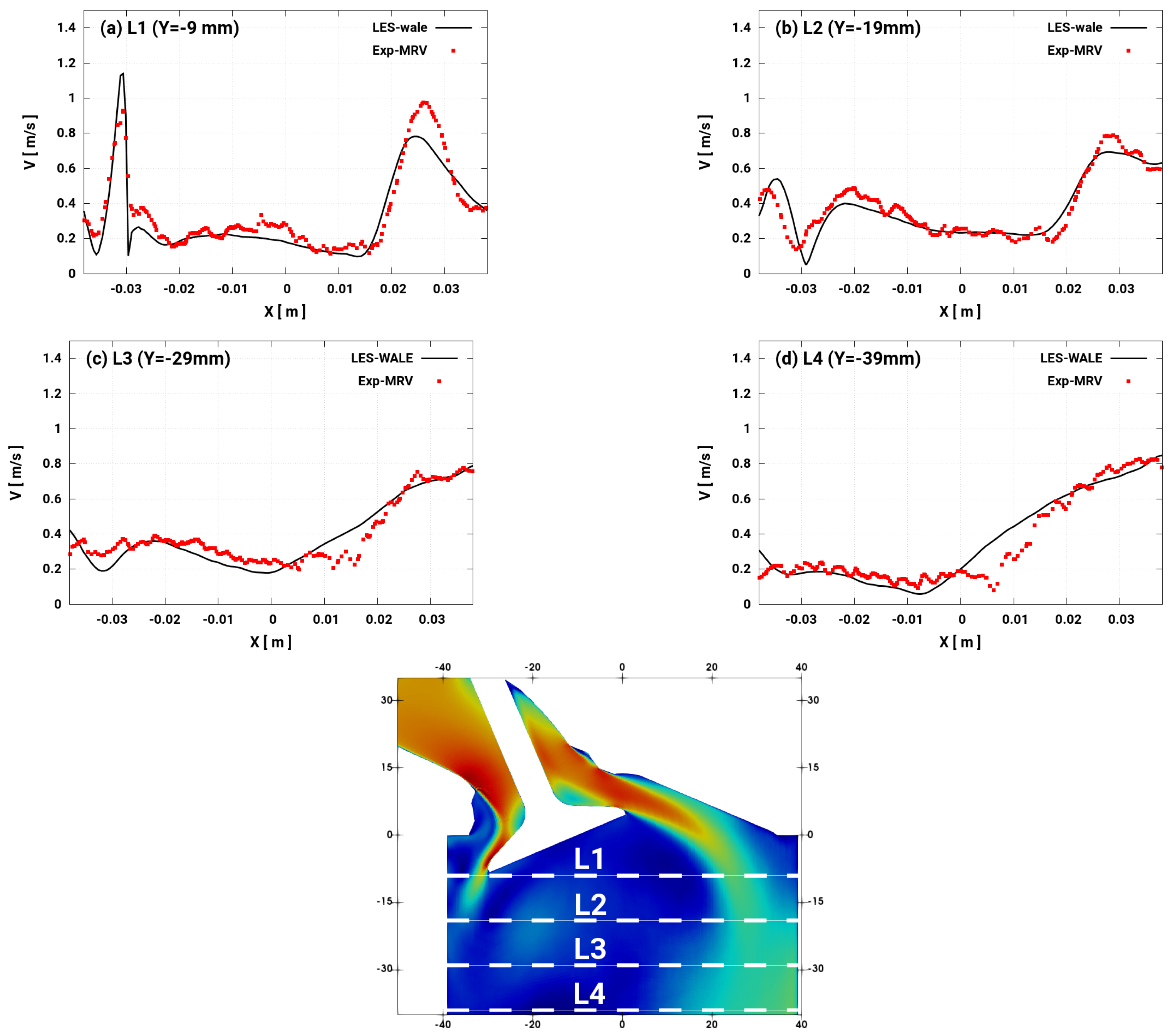
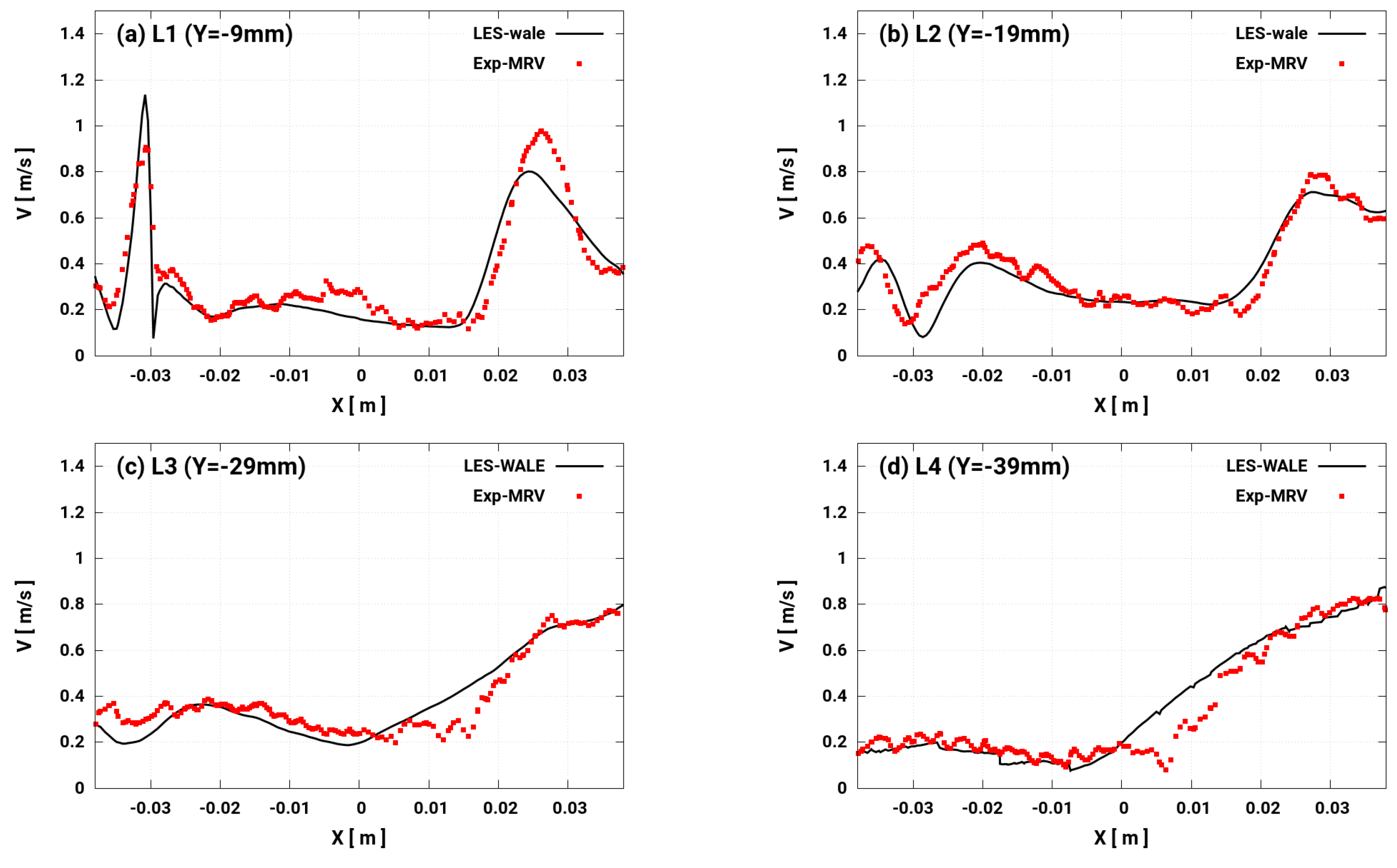
• using the WALE model based on the cost-accuracy criteria, the turbulent flow across the valve curtain clearly featured a back flow resulting in high speed intake jet at the middle. The averaged velocity results showed excellent agreement between LES and MRV measurement revealing the high prediction capability of the suggested LES tool for valve flows.
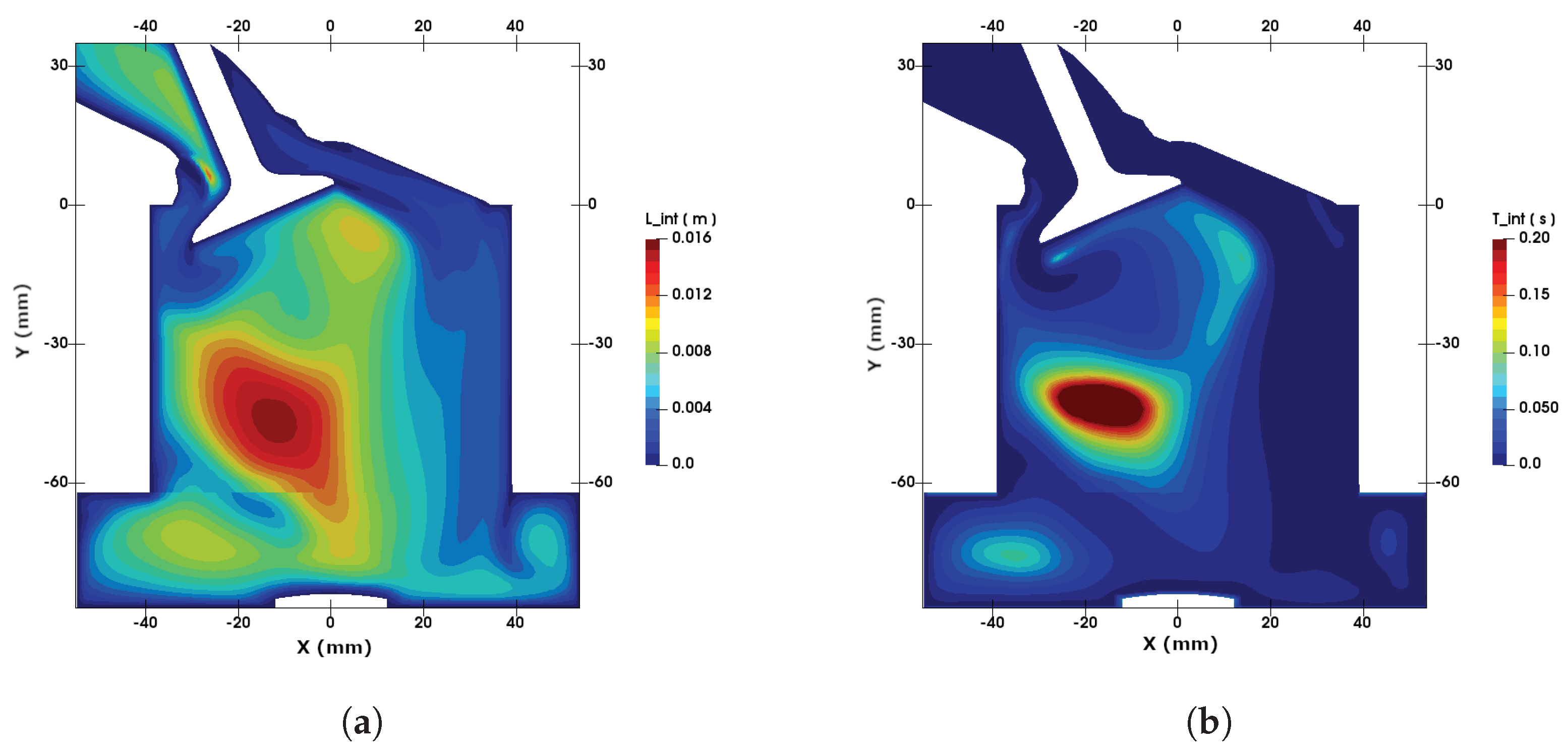
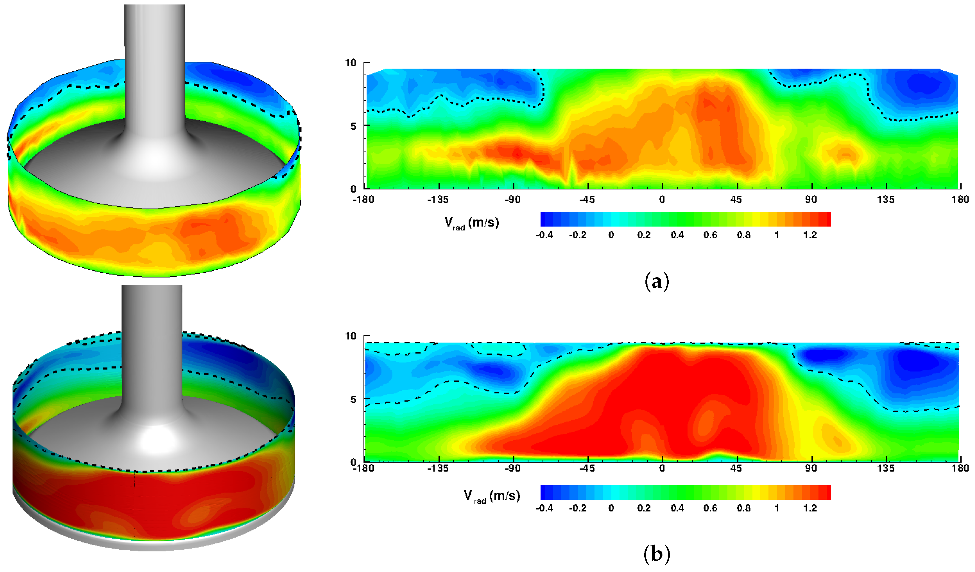
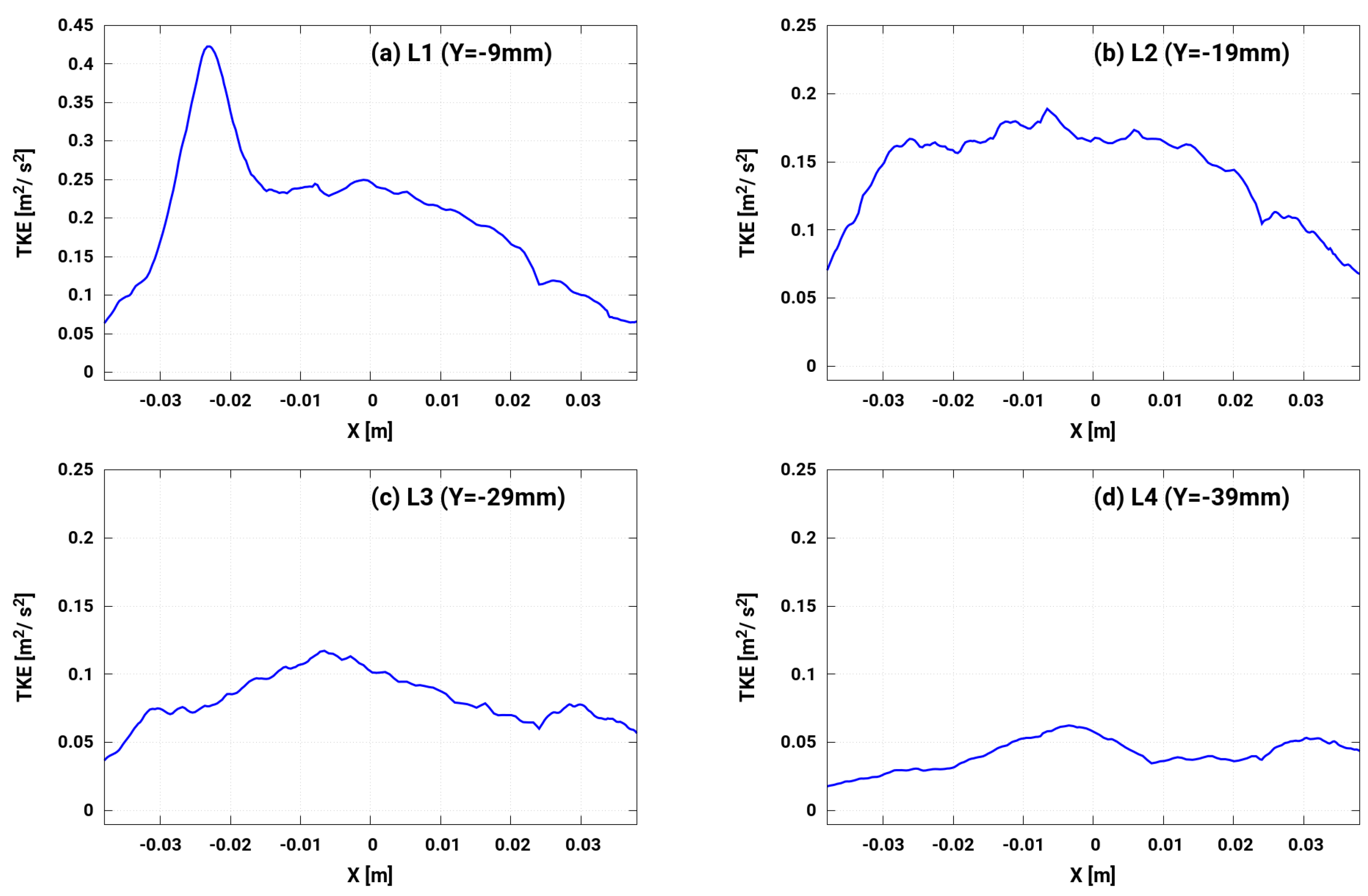
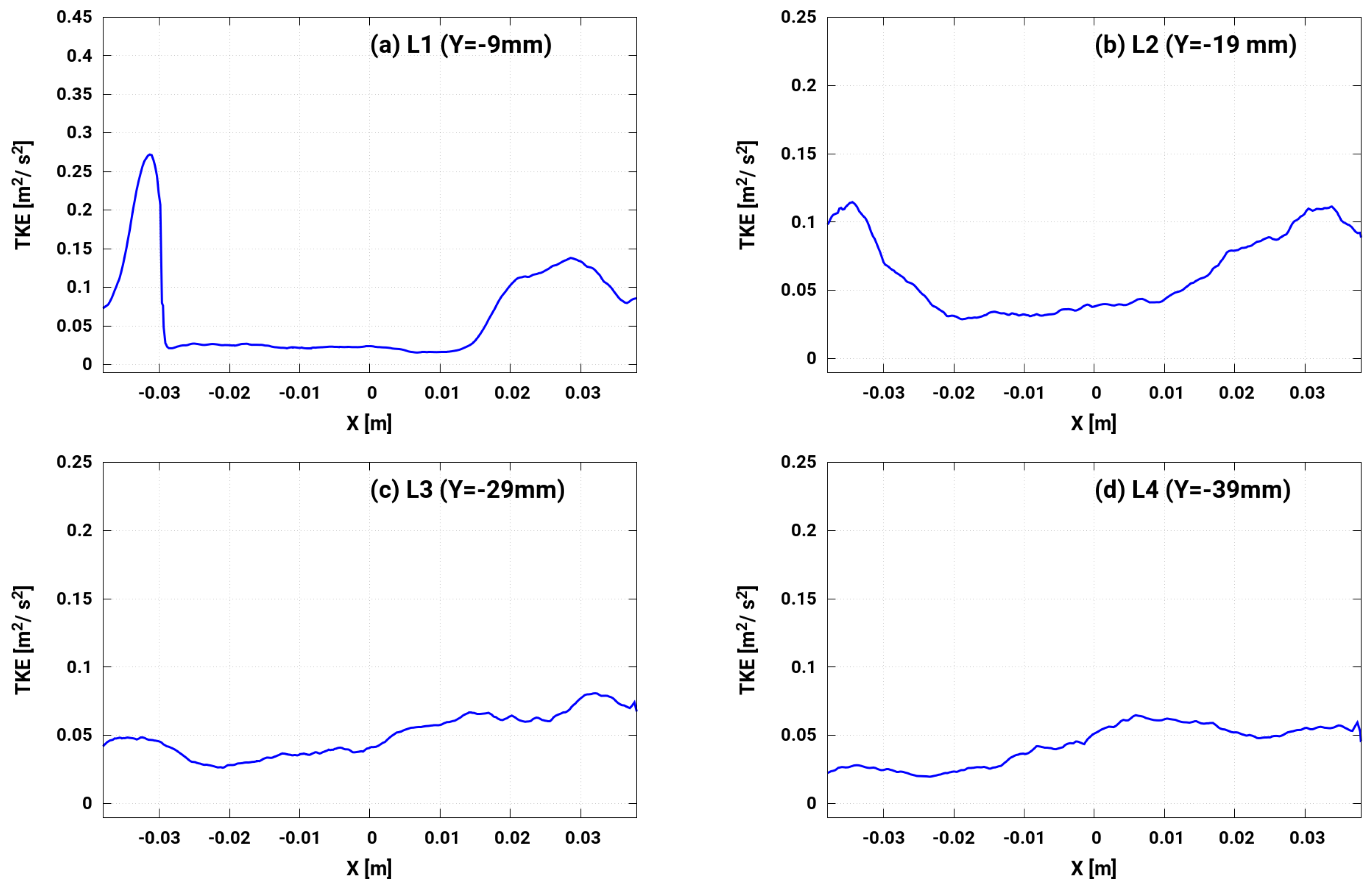
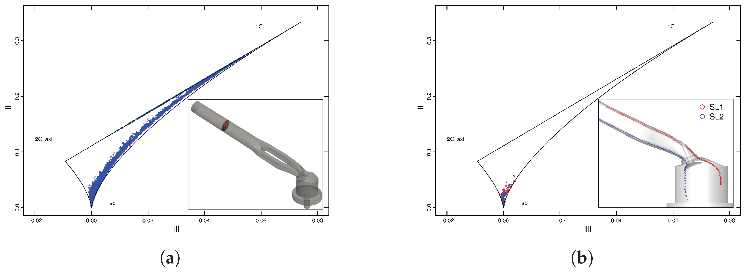
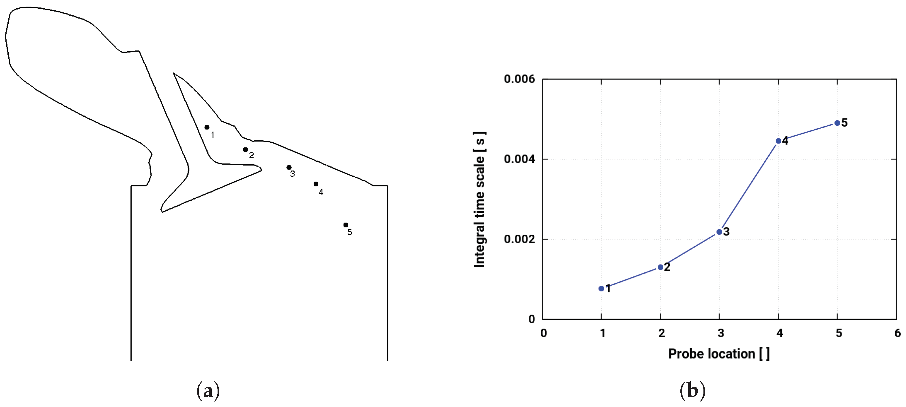
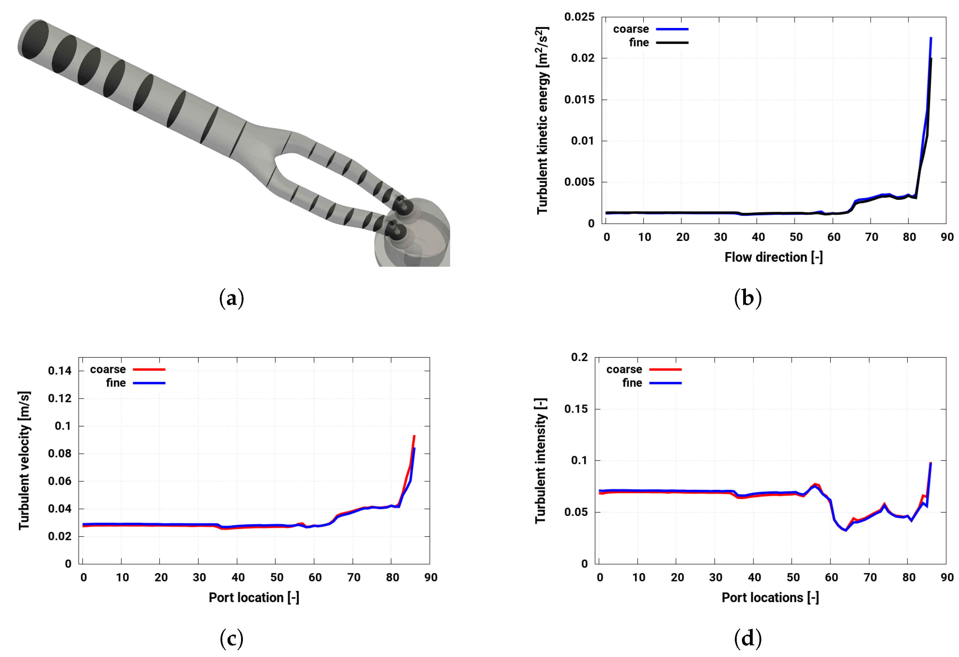
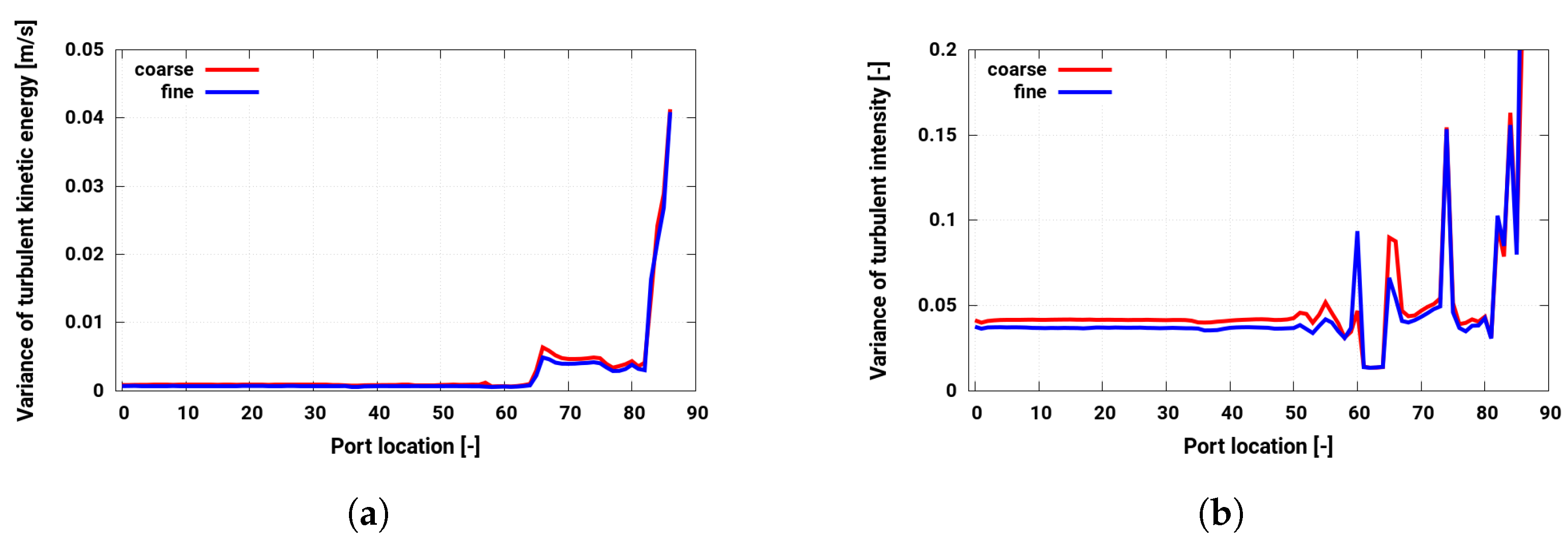
• physically, for the in-cylinder turbulent flow and for the intake port part, the turbulence and statistical analysis provided by LES led to some additional valuable findings. First, the flow anisotropy along the intake valve has been detected by means of an anisotropy map. Next, the integral turbulent scales along the intake-charge stream suggested a gradual increment of turbulent length scale downstream. Third, the evolution of turbulence properties along the port length showed that the most of the turbulence are generated across the valve passage and are mainly responsible for in-cylinder turbulence.

The presented methods will be further used to analyze the flow-bench configuration, representing the spray-guided engine in order to compare the results with those from the wall-guided configuration. Of note is that the evaluated methodology is ultimately to be used in a real engine configuration including valve and piston dynamics together with combustion process.

References

1. Heywood, J.B. Internal Combustion Engines Fundamentals; McGraw-Hill Publications: Hoboken, NJ, USA, 1989. [Google Scholar]
2. Bicen, A.; Vafidis, C.; Whitelaw, J. Steady and unsteady airflow through the intake valve of a reciprocating engine. J. Fluids Eng. 1985, 107, 413–420. [Google Scholar] [CrossRef]
3. Desantes, J.M.; Benajes, J.; Urchueguia, J. Evaluation of the non-steady flow produced by intake ports of direct injection Diesel engines. Exp. Fluids 1995, 19, 51–60. [Google Scholar]
4. Fukutani, I.; Watanabe, E. Air Flow through Poppet Inlet Valves—Analysis of Static and Dynamic Flow Coefficients; SAE Technical Paper; SAE International: Troy, MI, USA, 1982; p. 820154. [Google Scholar]
5. Towers, D.P.; Towers, C.E. Cyclic variability measurements of in-cylinder engine flows using high-speed particle image velocimetry. Meas. Sci. Technol. 2004, 15, 1917–1925. [Google Scholar] [CrossRef]
6. Drake, M.; Fansler, T.D.; Lippert, A.M. Stratified-charge combustion: Modeling and imaging of a spray-guided direct-injection spark-ignition engine. Int. J. Engine Res. 2005, 30, 2683–2691. [Google Scholar] [CrossRef]
7. Drake, M.; Haworth, D. Advanced gasoline engine development using optical diagnostics and numerical modeling. Proc. Combust. Inst. 2007, 32, 99–124. [Google Scholar] [CrossRef]
8. Fansler, T.D.; Reuss, D.L.; Sick, V.; Dahms, R.N. Invited Review: Combustion instability in spray-guided stratified-charge engines: A review. Int. J. Engine Res. 2015, 16, 260–305. [Google Scholar] [CrossRef]
9. Stiehl, R.; Bode, J.; Schorr, J.; Krüger, C.; Dreizler, A.; Böhm, B. Influence of intake geometry variations on in-cylinder flow and flow–spray interactions in a stratified direct-injection spark-ignition engine captured by time-resolved particle image velocimetry. Int. J. Engine Res. 2016, 17, 983–997. [Google Scholar] [CrossRef]
10. Church, W.; Farrell, P. Effects of Intake Port Geometry on Large Scale In-Cylinder Flows; SAE Technical Paper; lSAE International: Troy, MI, USA, 1998; p. 980484. [Google Scholar]
11. Justham, T.; Jarvis, S.; Clarke, A.; Garner, C.; Hargrave, G.K.; Halliwell, N. Simultaneous study of intake and in-cylinder IC engine flow fields to provide an insight into intake induced cyclic variations. J. Phys. Conf. Ser. 2006, 45, 146–153. [Google Scholar]
12. Freudenhammer, D.; Peterson, B.; Ding, C.; Böhm, B.; Jung, B.; Grundmann, S. The influence of cylinder head geometry variations on the volumetric intake flow captured by magnetic resonance velocimetry. SAE Int. 2015, 8, 1826–1836. [Google Scholar] [CrossRef]
13. Hartmann, F.; Buhl, S.; Gleiss, F.; Barth, P.; Schild, M.; Kaiser, S.A.; Haase, C. Spatially resolved experimental and numerical investigation of the flow through the intake port of an internal combustion engine. Oil Gas Sci. Technol. Rev. IFP Energies Nouvelles 2016, 71, 1–15. [Google Scholar] [CrossRef]
14. Freudenhammer, D.; Baum, E.; Peterson, B.; Böhm, B.; Jung, B.; Grundmann, S. Volumetric intake flow measurement of an IC engine using magnetic resonance velocimetry. Exp. Fluids 2014, 55, 1724. [Google Scholar] [CrossRef]
15. Freudenhammer, D.; Baum, E.; Peterson, B.; Böhm, B.; Grundmann, S. Towards time-resolved magnetic resonance velocimetry for IC-engine intake flows. In Proceedings of the 17th International Symposium of Applications of Laser Techniques to Fluid Mechanics, Lisbon, Portugal, 7–10 July 2014. [Google Scholar]
16. Baum, E.; Peterson, B.; Böhm, B.; Dreizler, A. On the validation of LES applied to internal combustion engine flows: Part 1: Comprehensive experimental database. Flow Turbul. Combust. 2014, 92, 269–299. [Google Scholar] [CrossRef]
17. Yin, C.; Zhang, Z.; Sun, Y.; Sun, T.; Zhang, R. Steady and unsteady airflow through the intake valve of a reciprocating engine. Eng. Appl. Comput. Fluid Mech. 2016, 10, 312–330. [Google Scholar]
18. Nishad, K. Modeling and Unsteady Simulation of Turbulent Multi-Phase Turbulent Flow Including Fuel Injection in IC-Engines. Ph.D. Thesis, Darmstadt University of Technology, Darmstadt, Germany, 2013. [Google Scholar]
19. Schmitt, M.; Frouzakis, C.E.; Tomboulides, A.G.; Wright, Y.M.; Boulouchos, K. Direct numerical simulation of multiple cycles in a valve/piston assembly. Phys. Fluids 2014, 26, 1–26. [Google Scholar]
20. Vermorel, O.; Richard, S.; Colin, O.; Angelberger, C.; Benkenida, A.; Veynante, D. Towards the understanding of cyclic variability in a spark ignited engine using multi-cycle LES. Combust. Flame 2007, 156, 1525–1541. [Google Scholar] [CrossRef]
21. Goryntsev, D.; Sadiki, A.; Klein, M.; Janicka, J. Large eddy simulation based analysis of the effects of cycle-to-cycle variations on air-fuel mixing in realistic DISI engines. Proc. Combust. Inst. 2009, 32, 2759–2766. [Google Scholar] [CrossRef]
22. Enaux, B.; Granet, V.; Vermorel, O.; Lacour, C.; Thobois, L.; Dugué, V.; Poinsot, T. Large eddy simulation of a motored single-cylinder piston engine: numerical strategies and validation. Flow Turbul. Combust. 2010, 86, 153–177. [Google Scholar]
23. Granet, V.; Vermorel, O.; Lacour, C.; Enaux, B.; Dugué, V.; Poinsot, T. Large-Eddy Simulation and experimental study of cycle-to-cycle variations of stable and unstable operating points in a spark ignition engine. Combust. Flame 2012, 159, 562–1575. [Google Scholar] [CrossRef]
24. Goryntsev, D.; Nishad, K.; Sadiki, A.M.; Janicka, J. Application of LES for analysis of unsteady effects on combustion processes and misfires in DISI engine. Oil Gas Sci. Technol. Revue d’IFP Energies Nouvelles 2014, 69, 129–140. [Google Scholar] [CrossRef]
25. Sadiki, A.; Di Mare, F.; Nishad, K.; Keller, P.; Stefan, B.; Hartmannand, F.; Hasse, C. Internal Combustion Engine. In Ercoftac best Practice Guidlines: Computational Fluid Dynamics of Turbulent Combustion; Chapter 5; Vervisch, L., Roekaerts, D., Eds.; Ercoftac: European Research Community on Flow, Turbulence and Combustion: London, UK, 2015. [Google Scholar]
26. Smagorinsky, J. General circulation experiments with primitive equations. Mon. Weather Rev. 1963, 91, 99–164. [Google Scholar] [CrossRef]
27. Nicoud, F.; Ducros, F. Subgrid-scale stress modelling based on the square of the velocity gradient tensor. Flow Turbul. Combust. 1999, 62, 183–200. [Google Scholar] [CrossRef]
28. Janicka, J.; Sadiki, A. Large eddy simulation of turbulent combustion systems. Proc. Combust. Inst. 2005, 30, 537–547. [Google Scholar] [CrossRef]
29. Pitsch, H. Large-eddy simulation of turbulent combustion. Annu. Rev. Fluid Mech. 1999, 38, 453–482. [Google Scholar] [CrossRef]
30. Rutland, C. Large eddy simulations for internal combustion engines - a review. Int. J. Engine Res. 2011, 12, 421–451. [Google Scholar] [CrossRef]
31. Keskinen, J.; Vuorinen, V.; Larmi, M. Large Eddy Simulation of the Intake Flow in a Realistic Single Cylinder Configuration; SAE Technical Paper; SAE International: Troy, MI, USA, 2012. [Google Scholar]
32. Thobois, L.; Rymer, G.; Souleres, T.; Poinsot, T.; Van den Heuvel, B. Large-Eddy Simulation for the Prediction of Aerodynamics in IC Engines. Int. J. Veh. Des. 2005, 39, 368–382. [Google Scholar] [CrossRef]
33. The OpenFOAM Foundation. OpenFOAM Programmer’s Guide, 2.4.0 ed.; The OpenFOAM Foundation: London, UK, 2015. [Google Scholar]
34. Ries, F.; Nishad, K.; Dressler, L.; Janicka, J.; Sadiki, A. Evaluating large eddy simulation results based on error analysis. Theor. Comput. Fluid Dyn. 2018, 1–20. [Google Scholar] [CrossRef]
35. Spalding, D.B. A single formula for the “law of the wall”. J. Appl. Mech. 1961, 28, 455–458. [Google Scholar] [CrossRef]
36. Klein, M.; Sadiki, A.; Janicka, J. A digital filter based generation of inflow data for spatially developing direct numerical or large eddy simulations. J. Comput. Phys. 2003, 186, 652–665. [Google Scholar] [CrossRef]
37. Kempf, A.; Klein, M.; Janicka, J. Efficient generation of initial- and inflow-conditions for transient turbulent flows in arbitrary geometries. Flow Turbul. Combust. 2005, 74, 67–84. [Google Scholar] [CrossRef]
38. Zagarola, M.; Perry, A.; Smits, A. Log laws or power laws: The scaling in the overlap region. Phys. Fluids 1997, 9, 2094–2100. [Google Scholar] [CrossRef] [Green Version]
39. Lund, T.; Wu, X.; Squires, K. Generation of turbulent inflow data for spatially-developing boundary layer simulations. J. Comput. Phys. 1998, 140, 233–258. [Google Scholar] [CrossRef]
40. Launder, B.; Spalding, D.B. The numerical computation of turbulent flows. Comput. Methods Appl. Mech. Eng. 1974, 3, 269–289. [Google Scholar] [CrossRef]
41. Oberkampf, W.; Roy, C.J. Verification and Validation in Scientific Computing; Cambridge University Press: Camnridge, UK, 2010. [Google Scholar]
42. Lumley, J.; Newman, G. The return to isotropy of homogeneous turbulence. J. Fluid Mech. 1977, 82, 161–178. [Google Scholar] [CrossRef] [Green Version]
Figure 1. Magnetic resonance velocimetry (MRV) flow bench configuration [15].
Energies 12 02620 g001
Figure 2. Computational domain with fully hex-hedral grid examplarily showing the coarse mesh with ≈4.9 millions CVs (control volumes). Note that the fine mesh amount ≈39 millions CVs.
Energies 12 02620 g002
Figure 3. Integral length and time scales evaluated along one of the valve plane using k- ε model based simulation. (a) Integral length scale; (b) Integral time scale.
Energies 12 02620 g003
Figure 4. Evolution of normalized absolute error (nAE) for in-cylinder flow against MRV(Magnetic resonance velocimetry) data for various turbulence models. (a) WALE (fine mesh); (b) WALE (coarse mesh); (c) RANS (coarse mesh); (d) Dynamic one equation (coarse mesh); (e) SIGMA model (coarse mesh); (f) Smagorinsky Model (coarse mesh).
Energies 12 02620 g004
Figure 5. Comparison of normalized mean absolute error (nMAE) of velocity against MRV(Magnetic resonance velocimetry) data for various turbulence models.
Energies 12 02620 g005
Figure 6. Comparison of velocity contour across mid-valve position in tumble plane ( Z = 19 mm): velocity evolution in intake-valve-passage and engine-cylinder. (a) MRV [15]; (b) LES-WALE.
Energies 12 02620 g006
Figure 7. Comparison of velocity contour across both intake valves ( X = 10 mm) in cross-tumble plane: complex flow structure between both valves and valve-cylinder wall. (a) MRV [15]; (b) LES-WALE.
Energies 12 02620 g007
Figure 8. Comparison of velocity contour in swirl plane below the intake ports (Y = −10 mm). (a) MRV [15]; (b) LES-WALE.
Energies 12 02620 g008
Figure 9. Comparison of velocity profile at valve curtain. (a) MRV [15]; (b) LES-WALE.
Energies 12 02620 g009
Figure 10. Comparison of velocity profile for LES and MRV across plane at Z = 0 mm along various lines as represented in the bottom figure.
Energies 12 02620 g010
Figure 11. Comparison of velocity profile for LES and MRV at various locations on plane at Z = 19 mm along various lines as represented in the bottom figure.
Energies 12 02620 g011
Figure 12. Comparison of velocity profile for LES and MRV at various locations (see Figure 11) on plane at Z = 19 mm).
Energies 12 02620 g012
Figure 13. Turbulent kinetic energy profile at various locations (see Figure 10, bottom) on the middle plane at Z = 0 mm.
Energies 12 02620 g013
Figure 14. Turbulent kinetic energy profile at various locations (see Figure 11, bottom) on a plane at Z = 19 mm.
Energies 12 02620 g014
Figure 15. Anisotropy map of intake valve flow: (a) across the duct plane, (b) along the stream lines.
Energies 12 02620 g015
Figure 16. Evolution of integral time scale along charge intake stream: (a) probe locations, (b) integral time scale.
Energies 12 02620 g016
Figure 17. Evolution of turbulence properties along the intake duct: (a) schematic of part of the cross-sectional locations along intake duct to carry out turbulence analysis, (b) turbulent kinetic energy, (c) turbulent velocity, (d) turbulence intensity.
Energies 12 02620 g017
Figure 18. Evolution of variance of turbulence properties along the intake duct: (a) variance of turbulent kinetic energy, (b) turbulence intensity.
Energies 12 02620 g018
Figure 19. Turbulence properties from LES (WALE -fine mesh) along the valve curtain: (a) absolute mean velocity, (b) turbulent kinetic energy, (c) turbulent velocity, (d) turbulence intensity.
Energies 12 02620 g019