CFD Simulation of Defogging Effectivity in Automotive Headlamp

Abstract

In the past decade, the condensation of internal air humidity in automotive headlamps has become more prevalent than ever due to the increased usage of a new light source—LEDs. LEDs emit far less heat than previously-used halogen lamps, which makes them far more susceptible to fogging. This fogging occurs when the internal parts of the headlamp fall to a temperature below the dew point. The front glass is most vulnerable to condensation due to its direct exposure to ambient conditions. Headlamp fogging leads to a decrease in performance and the possibility of malfunctions, which has an impact not only on the functional aspect of the product’s use but also on traffic safety. There are currently several technical solutions available which can determine the effectivity of ventilation systems applied for headlamp defogging. Another approach to this problem may be to use a numerical simulation. This paper proposes a CFD (computational fluid dynamics) simulation with a slightly simplified 3D model of an actual headlamp, which allows simulation of all the phenomena closely connected with fluid flow and phase change. The results were validated by real experiments on a special fogging–defogging test rig. This paper compares three different simulations and their compliance with real experiments.

1. Introduction

Car headlamps serve two practical purposes: to see and to be seen. It is important that the headlamps’ proper functionality is guaranteed in all conditions, otherwise the risk of an accident is increased. Car manufacturers have to create headlamps that are able to work flawlessly in all weather conditions, from hot summer days when the sun is shining to very cold temperatures when the temperature difference between the car and the air is high.

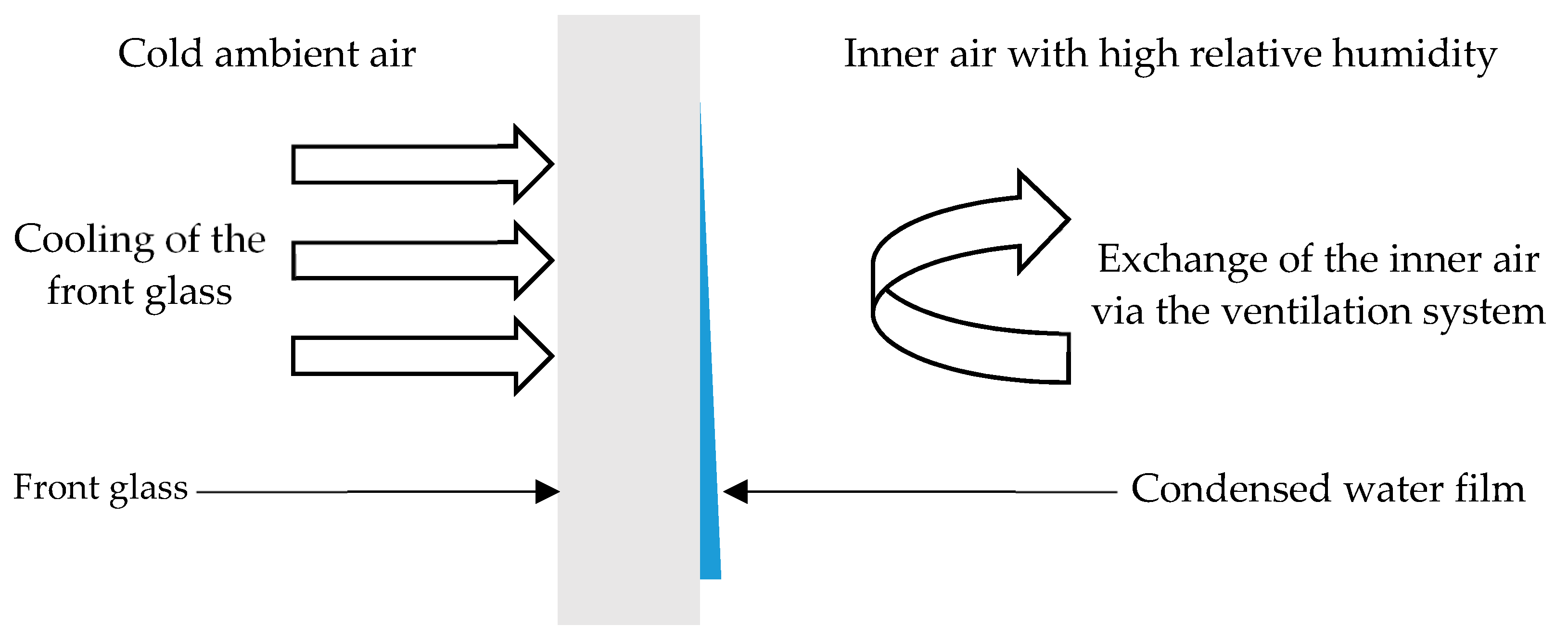
The second extreme can lead to the problem of dew inside the headlamp, which limits the headlamp’s illumination. This dew is created mainly on the front glass, because of the high temperature difference, and it occurs when the glass’ temperature decreases to below the dew point of the inside air.

This fogging happens due to the moisture, which can find its way inside the headlamp via these three mechanisms [1]:

• Sorption of plastic components—every plastic material is able to absorb a certain amount of ambient moisture, which may later be released when the thermal conditions change;
• Permeation of water vapor through housing and lens material—materials traditionally used for the headlamps are not completely impermeable to the water vapor;
• Moisture transferred via the venting system—the venting system serves to change the air inside the headlamps, which helps to reduce the amount of fogging by transporting in warmer air. This system may also bring in air with higher humidity, which can later lead to the undesirable fogging.

This problem occurs much more today than it used to because of the increasing trend in LED headlamp technology. It will still be prevalent even with future technologies such as laser headlamps [2].

LEDs allow car manufacturers to create new, previously impossible headlamp designs and to have a larger range of styles, which has proven popular among customers. However, one of their downsides in comparison with previously used halogen lamps is that they radiate only a fraction of the heat. While halogen lamps would heat the front glass via infrared radiation, the waste heat created in LEDs is mainly conducted away into heat sinks which are placed in the back of the lamp or even outside. This property makes the front glass of the new lamps more prone to fogging. Approximately 35% of customers’ complaints about LED headlamps are connected to headlamp fogging [1].

All headlamps have a ventilation system. This system is composed of openings in the back of the headlamp, which allow air exchange. Their positions are chosen based on the drive tests or numerical simulations at places with the highest pressure differences to ensure the best airflow. Currently, various technical solutions exist to help basic ventilation:

• Ventilation system with membranes—diffusive transfer of moisture from the headlamp. Pros: long-term solution, no dust ingress. Cons: reduces the airflow through the ventilation system.
• Anti-fog coating—prevents the formation of water droplets. Pros: works all the time. Cons: limited lifetime, does not remove moisture.
• Non-regenerable desiccant bags—absorb the moisture. Pros: simple solution, works all the time. Cons: limited lifetime.
• Fans—blow the waste heat from LEDs to other parts of the headlamp. Pros: long-term solution. Cons: works only when the vehicle is active, does not remove moisture.

This paper looks at a CFD (computational fluid dynamics) simulation of defogging of the front glass through air exchange via the headlamp’s ventilation system.

2. Problem Description

If headlamps do not possess a fan to further cool down the LEDs, the two predominant phenomena occurring are natural convection and phase change of water. The principles of natural convection inside cavities such as headlamps have already been studied in detail [3,4,5]. Unfortunately, the phase change of moisture brings additional challenges to the simulation. These problems have not been studied deeply enough in the case of headlamps, but there is various research where windshield fogging has been studied [6,7]. There have also been studies solving the combination of natural convection and radiation inside car headlamps [8]. The study done in [9] dealt with the same complexities of the problem, but only simulated a simple box that stood in for the headlamp.

This study solves a simulated problem of real 3D headlamp geometry, not including thermal radiation. A turned-off-headlamp simulation was conducted in order to observe the influence of the vent system without any additional heating (worst-case scenario). The simulation was carried out using the commercially available software ANSYS FLUENT. The phase change of the dew was solved by using the Eulerian wall film (EWF) approach—the same approach used in [9].

3. Experiment on Fogging–Defogging Test Rig

A special method for the fogging and defogging of car headlamps was developed in the Heat Transfer and Fluid Flow Laboratory at Brno University of Technology, Faculty of Mechanical Engineering.

The standard testing procedure often uses climatic chambers [10] to create ambient conditions in which the headlamp fogs. These methods often take many hours to create the fogging effect because the first part of moisture absorption is achieved by creating hot ambient air with a relatively high humidity to allow the plastic materials to take in as much of the moisture as they can, which is a slow process. The ambient air is then cooled down to desorb water and create condensation inside the headlamp. The exact amount of condensed water and its layout is unknown, which makes this process difficult to simulate. Furthermore, these tests often do not put any pressure on the ventilation holes, and the influence on the vehicle’s movement is therefore unknown.

The method we developed is based on evaporating moisture inside the headlamp’s body, which immediately creates internal air with high humidity, while only the front glass is cooled down, for the dew to condense primarily there. This approach is much faster and cheaper than conventional methods, because the fogging of the headlamp only takes less than thirty minutes and there is no need for a special thermal chamber to create conditions in which the dew would be slowly formed in the measured headlamp. For this reason, this approach can theoretically be used even in a real drive test.

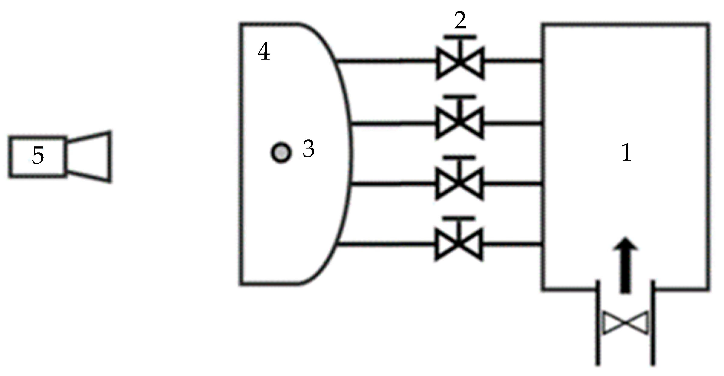
The core component of this method is a specially developed humidifier which is inserted inside the headlamp. By boiling a specified amount of water stored inside, the lamp’s internal air becomes more humid. The schematic of the test rig is shown in Figure 1.

The experiment consisted of two main parts. The first, preparative, stage of the experiment is the fogging of the headlamps. A specified amount of water was evaporated into the headlamp’s body while the front glass was being cooled. The evaporation process was monitored by checking the internal air humidity. The initial stage ended when all the water vapor condensed on the front glass.

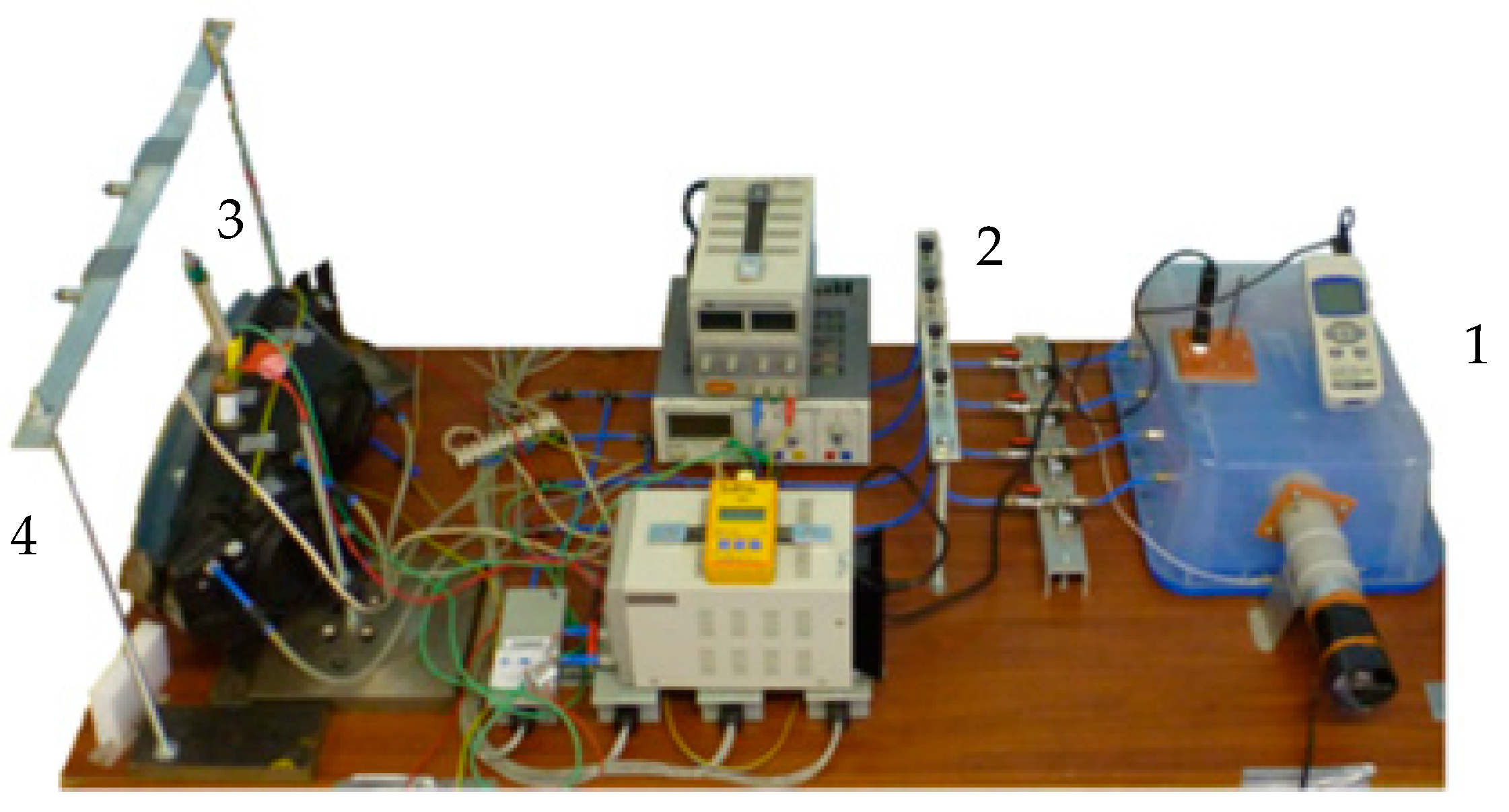
The second phase of the experiment was the defogging. In this stage, specific pressures were created on the ventilation holes to simulate the pressure gradient of a moving vehicle. Air exchange is achieved thanks to the generated pressure gradients, leading to the defogging. The process of defogging was monitored by a camera which took pictures in a specific time-step. The temperature and humidity of the ambient air were monitored to set the simulation’s boundary conditions. The actual testing rig is shown in Figure 2.

Glass temperature was measured by K-type thermocouples with an accuracy of ±1.5 °C, ambient temperature was measured by a Pt100 RTD temperature sensor with an accuracy of ±0.3 °C, and air humidity and internal temperature were measured by a thermometer/hygrometer data logger RHXL3SD with an accuracy of ±0.8 °C for the measurement of temperature and ±3% for the measurement of humidity. The measured data were collected by National Instruments hardware, and the experiments were carried out by the commercially available software LabVIEW.

4. Numerical Simulation Setup

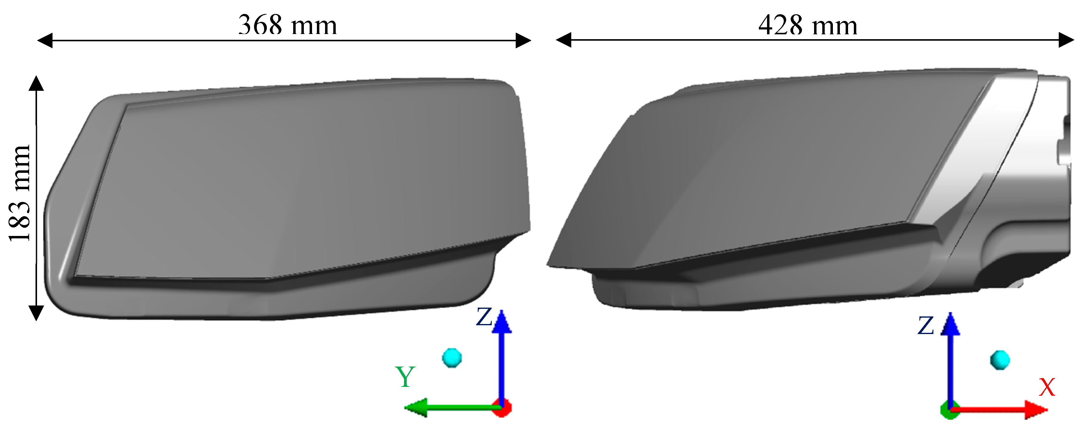
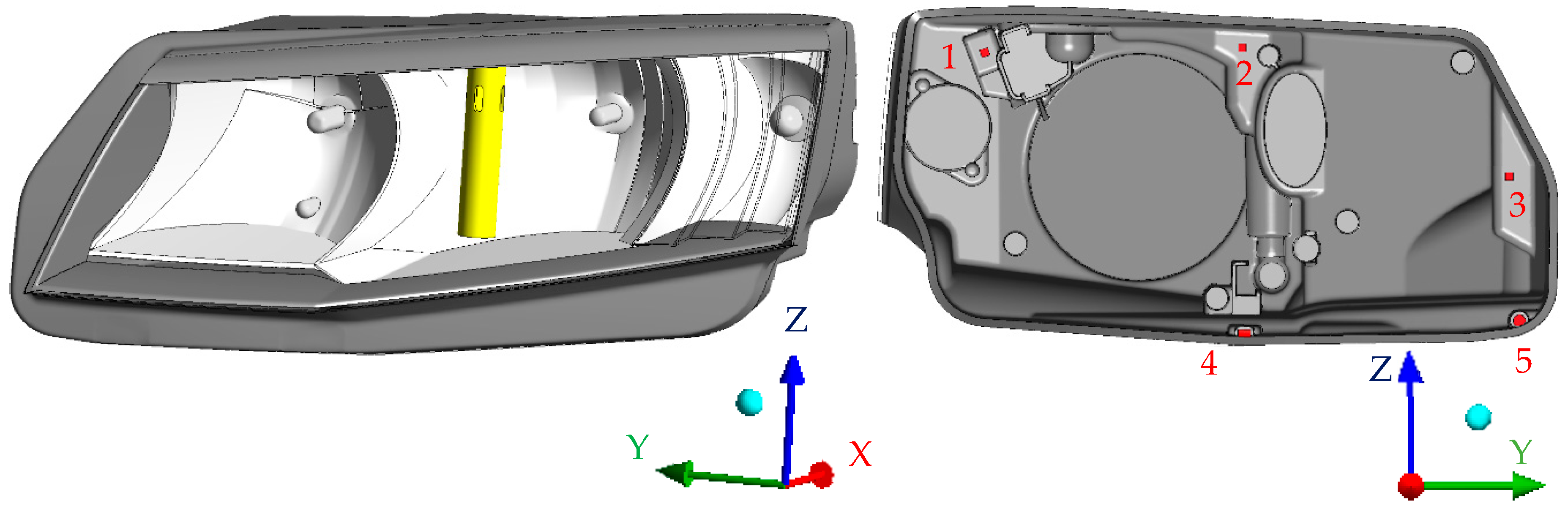
Modern car headlamps have a very complex topology consisting of LED chips, heat sinks, optical features, control mechanisms for directing the light, and an inner construction that holds it all together. For this reason, a simplified headlamp model would not give reliable results and therefore an original 3D model of the headlamp with minimal simplifications was used. The main dimensions of the headlamp used are shown in Figure 3. The glass’ thickness was 2.9 mm. Figure 4 shows the inside of the headlamp with the humidifier (left) and the positions of the ventilation holes (right). The humidifier was a cylindrical body with diameter 20 mm and height 115 mm.

The numerical simulation was composed of the inner headlamp space (fluid domain), front glass (solid domain), and humidifier (solid domain). The material of the front glass was polycarbonate, with a specific heat of 1132.2 J∙kg⁻¹∙K⁻¹ and thermal conductivity defined by Equation (1):

$$k=0.002947·T+0.3197,$$

(1)

where $k$ is the thermal conductivity of the polycarbonate and $T$ is its temperature.

The entire case was excluded from the simulations because it would have only minimal importance to the results and would significantly enlarge the computational mesh. The front glass needed to be present to ensure realistic defogging time, which is dependent on the heat transfer with the surrounding air, determined by the glass’ width, specific heat, and thermal conductivity.

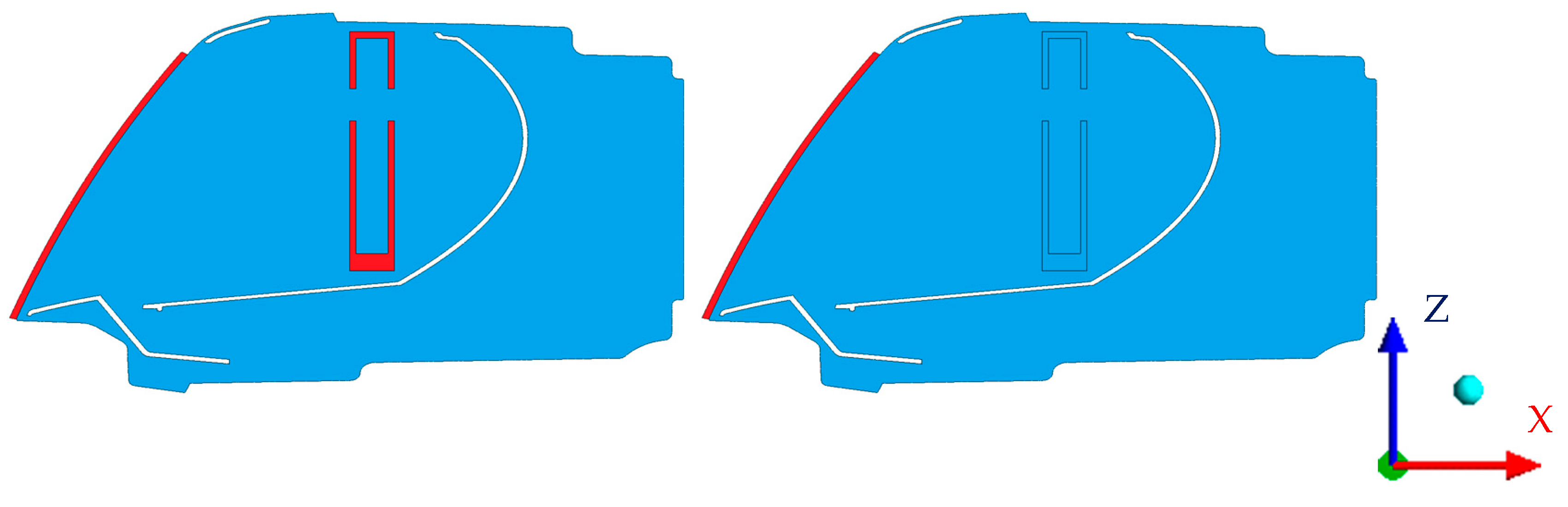
Figure 5 shows a cross section of the simulated domain. Red represents solid domains and blue represents fluid domains. White areas inside the headlamp are individual internal parts excluded from the computational mesh.

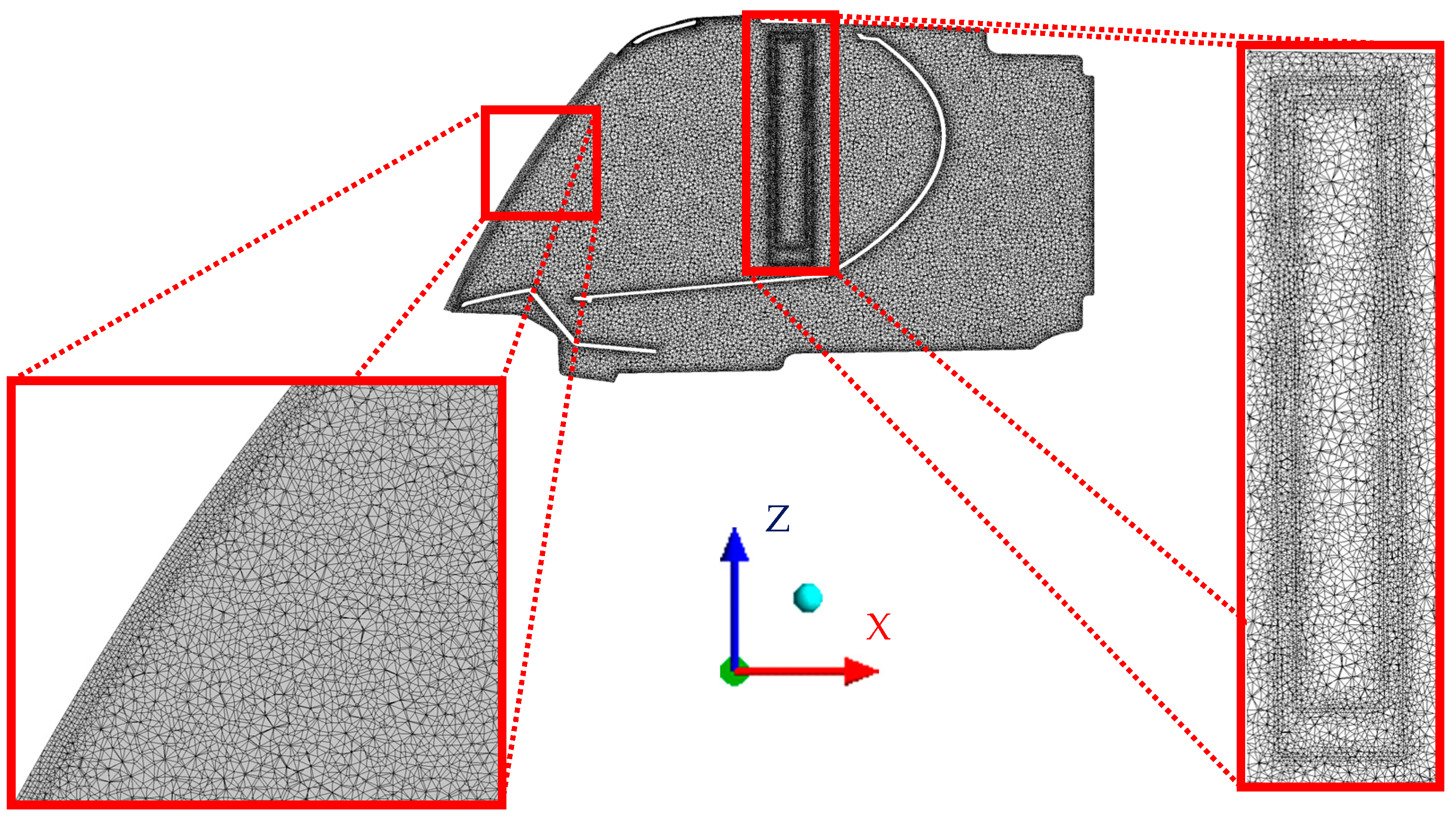
The original headlamp geometry was imported to ANSYS Fluent meshing to create the surface and volume mesh. Then, the humidifier was added to the geometry to simulate the fogging stage. The final mesh was composed of 17.5 million elements in total, of which 16.9 million were tetrahedral, 604,570 were wedges, and 456 were pyramids.

The cross section of the mesh is shown in Figure 6, where the areas around the humidifier and the front glass are shown in better detail.

The simulation was composed of two stages: fogging (preparative) and defogging (evaluated). Both were run in transient mode in order to capture the development of the fogging and defogging. The time step was 20 s, and the maximum number of iterations per time step was set to 50.

The maximal value of velocity near the glass was 0.08 m∙s⁻¹, the lowest air temperature was 4 °C, which has a kinematic viscosity of 1.36 × 10⁶ m²∙s⁻¹ [11], and the height of the headlamp glass was 0.16 m. They Reynolds number could be calculated from Equation (2):

$$Re=\frac{L·v}{\nu },$$

(2)

where $L$ is the characteristic length (glass height), $v$ is the air velocity, and $\nu$ is the kinematic viscosity. According to [12], the critical Reynolds number in the case of flow over a plate is 10⁵ and in this case the Reynolds number was equal to 9.4 × 10³, and therefore a turbulence model was not accounted for because the considered flow was in the laminar regime.

The fogging process was also simulated because a constant water film thickness would not give realistic results. A heterogeneous water film was needed to be created on the front glass with a similar thickness to the real situation. In this stage, the ventilation openings’ boundary conditions were set as walls. The mass flow rate of water vapor was a constant, calculated from the amount and total time needed for the evaporation in the case of experiments as shown in Equation (3), where $Q$ is the mass flow, $m$ is the total mass of evaporated water, and $t$ is the time needed for evaporation:

$$Q=\frac{m}{t}.$$

(3)

The mass diffusivity through the humidifier’s body was user-defined, dependent on the cells’ temperature and local pressure. For the last 5 min of this stage, the mass flow from the humidifier was turned off. This time served for the condensation of the remaining water vapor.

The second stage simulated the defogging itself, and the results obtained in this part were used for the overall comparison. The humidifier’s solid domain was changed to a liquid domain, and its boundaries were changed from walls to an interior. All but one of the ventilation openings’ boundaries were changed from walls to inlets with a set pressure of 60 Pa, while the remaining one was set as a pressure outlet. The glass and housing temperatures and all reference values were set according to the measured values from the experiment. The solver was set according to

Table 1. Models used. EWF: Eulerian wall film.

Model	Settings
Energy	On
Viscous	Laminar
Species	Species transport
EWF	On

.

For pressure–velocity coupling, the SIMPLE scheme was used and set according to

Table 2. Solution methods used.

Variable	Scheme
Gradient	Least squares cell-based
Pressure	Standard
Momentum	Second-order upwind
H2O	Second-order upwind
Energy	Second-order upwind
Transient formulation	Second-order implicit

.

Governing Equations

The condensation was solved by using the Eulerian wall film (EWF) approach. EWF is used for predicting the creation and flow of thin films of liquids on a surface. This approach assumes that the film thickness is much smaller than the radius of curvature of the surface, as shown in Figure 7. EWF allows only one condensable component, which was water in this simulation. For computing simulations with thin liquid layers, the volume of fluid method (VOF) can be used, but this approach has a high computational power demand. In our case, EWF was used for faster computation. The model we used neglects the change of heat transfer resistance by the liquid wall film.

Mathematical equations used in this approach:

The conservation of mass for a film in a 3D domain is given by Equation (4):

$$\frac{\partial h}{\partial t}+{𝛻}_s·\left[h{\overline{V}}_l\right]=\frac{\dot{m_s}}{{\rho }_l},$$

(4)

where ${\rho }_l$ is the liquid density, $h$ is the film height, ${𝛻}_s$ is the surface gradient operator, ${\overline{V}}_l$ is the mean film velocity, and $\dot{m_s}$ is the mass source per unit area due to droplet collection, film separation, film stripping, and phase change.

Conservation of film momentum is given by Equation (5):

$$\frac{\partial h\stackrel{\rightharpoonup }{{\overline{V}}_l}}{\partial t}+{𝛻}_s·\left(h\stackrel{\rightharpoonup }{{\overline{V}}_l}\stackrel{\rightharpoonup }{{\overline{V}}_l}\right)=-\frac{h{𝛻}_s{P}_L}{{\rho }_l}+\stackrel{\rightharpoonup }{g_{\tau }}h+\frac{3}{2{\rho }_l}{\overline{\tau }}_{fs}-\frac{3·{\nu }_l}{h}\stackrel{\rightharpoonup }{{\overline{V}}_l}+\frac{\dot{q}}{{\rho }_l},$$

(5)

where:

$$P_L=P_{gas}+P_h$$

(6)

and

$$P_h=-\rho h\left(\stackrel{\rightharpoonup }{n}·\stackrel{\rightharpoonup }{g}\right).$$

(7)

Conservation of energy is given as:

$$\frac{\partial \left(h{T}_f\right)}{\partial t}+{𝛻}_s·\left(\stackrel{\rightharpoonup }{{\overline{V}}_f}h{T}_f\right)=\frac{1}{\rho C_p}·\left\{2k_f\left[\frac{T_s+T_w}{h}-\frac{2T_f}{h}\right]+{\dot{q}}_{imp}+{\dot{m}}_{vap}L\left(T_s\right)\right\},$$

(8)

where $T_s$ is the temperature at the film–gas interface, $T_f$ is the average film temperature, $T_W$ is the wall temperature, ${\dot{q}}_{imp}$ is the source term, ${\dot{m}}_{vap}$ is the mass vaporization of the condensation rate, and $L\left(T_s\right)$ is the latent heat.

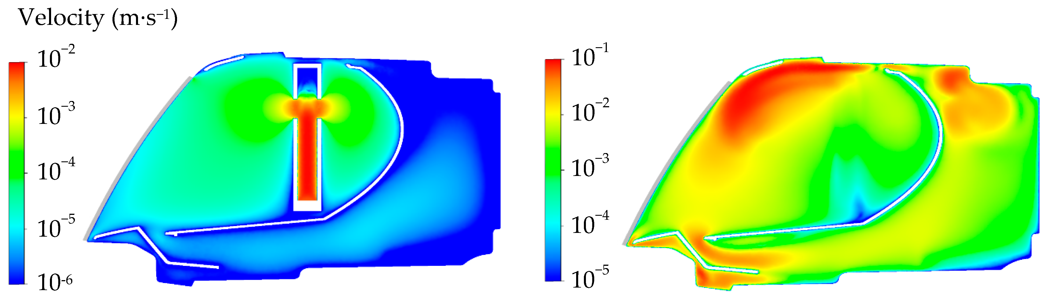
Figure 8 shows the velocity distributions in case of fogging and defogging in cross section through the humidifier with 2 mL of evaporated water. The left side shows the slow evaporation of water from the humidifier. The maximum velocity of the steam was 0.03 m∙s⁻¹, while the average velocity was 7 × 10⁻⁴ m∙s⁻¹. The right side shows air circulation inside the lamp during the defogging phase. In this cross section, the ventilation opening with the set pressure was at the top of the lamp. The maximum velocity was 0.18 m∙s⁻¹ and the average value was 0.02 m∙s⁻¹.

5. Results Comparison

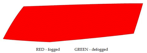
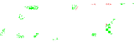
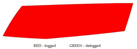
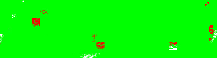
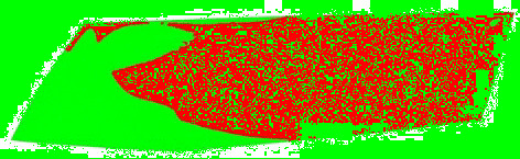
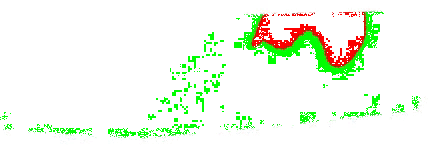
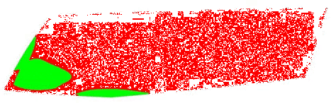
The dew thickness was monitored, and the results were shown only in two contours for better comparison with real-life experiments where the image processing showed only still-fogged and defogged areas. The image processing compared every image to two other images (fully fogged and fully defogged) and then decided if the area was fogged or already defogged.

The minimum dew thickness still considered as fogged was 0.1 nm, which is the minimal visible light scattering thickness [13].

Comparison of laboratory experiments and simulations was done by creating a time lapse of fogging and defogging from processed experiment photos and simulation results. Two significant moments were chosen: first for the time when 50% of the glass area became defogged, and then when 80% of the glass was defogged. Three different simulations and experiments were conducted that differentiated the amount of evaporated water inside the lamp.

Table 3. Initial conditions for the fogging phase simulation.

IC (Initial Conditions)	Setting	C1	C1.5	C2
Glass temperature (°C)	Set according to the experiment	20.3	23.2	24.4
Internal temperature (°C)	Set according to the experiment	22.1	21.9	22.5
Internal humidity (%)	Set according to the experiment	55.2	61.5	61.2

shows the initial conditions in simulating the fogging stage. These values were obtained during the real experiments.

The boundary condition was the mass flow inlet on the humidifier with a mass flow rate calculated according to the corresponding experiment. The constant mass fraction of water was equal to 0.99, and the temperature was 100 °C. The mass flow rates are shown in

Table 4. Mass flow rate and corresponding evaporation time in simulations.

Case	Evaporation Time (mm:ss)	Mass Flow Rate (×10−6 kg∙s)
C1	15:00	1.11
C1.5	22:30	1.11
C2	20:00	1.67

.

These values were set according to the experiments. During the experiments, the power input to the humidifier was controlled to achieve optimal internal humidity in order to ensure that the water vapor would condense only on the glass’ surface. This explains the longer time in C1.5 in comparison to C2.

The initial conditions (temperature and humidity distribution) in the defogging stage were set according to the previous fogging simulations.

Table 5. Boundary conditions for the defogging phase simulation.

BC (Boundary Conditions)	Setting	C1	C1.5	C2
Ambient air temperature (°C)	Set according to the experiment	23.1	21.0	27.0
Ambient air humidity (%)	Set according to the experiment	38.9	29.4	41.1
Ventilation opening 1 (Pa)	Pressure inlet, 60 Pa	60	60	60
Ventilation opening 2 (Pa)	Pressure inlet, 60 Pa	60	60	60
Ventilation opening 3 (Pa)	Pressure inlet, 60 Pa	60	60	60
Ventilation opening 4 (Pa)	Pressure inlet, 60 Pa	60	60	60
Ventilation opening 5	Pressure outlet	-	-	-
Heat transfer coefficient on the glass surface	Calculated according to Equation (9)	4.3	4.2	4.4

presents the boundary conditions for the defogging stage.

$$h=\frac{k_{air}}{L}·0.517·R{a}^{\frac{1}{4}},$$

(9)

where $h$ is the heat transfer coefficient, $k_{air}$ is the thermal conductivity of air (obtained from [11]), $L$ is the characteristic length (glass height), and $Ra$ is Rayleigh number which is equal to:

$$Ra=\frac{g·\beta ·\mathsf{\theta }·L^3}{\alpha ·\nu },$$

(10)

where $g$ is gravitational acceleration, $\beta$ is the volumetric expansion coefficient, $\mathsf{\theta }$ is the temperature difference between glass and ambient air, $\alpha$ is the thermal diffusivity, and $\nu$ is kinematic viscosity.

5.1. Comparison of Results C1—1 mL of Evaporated Water

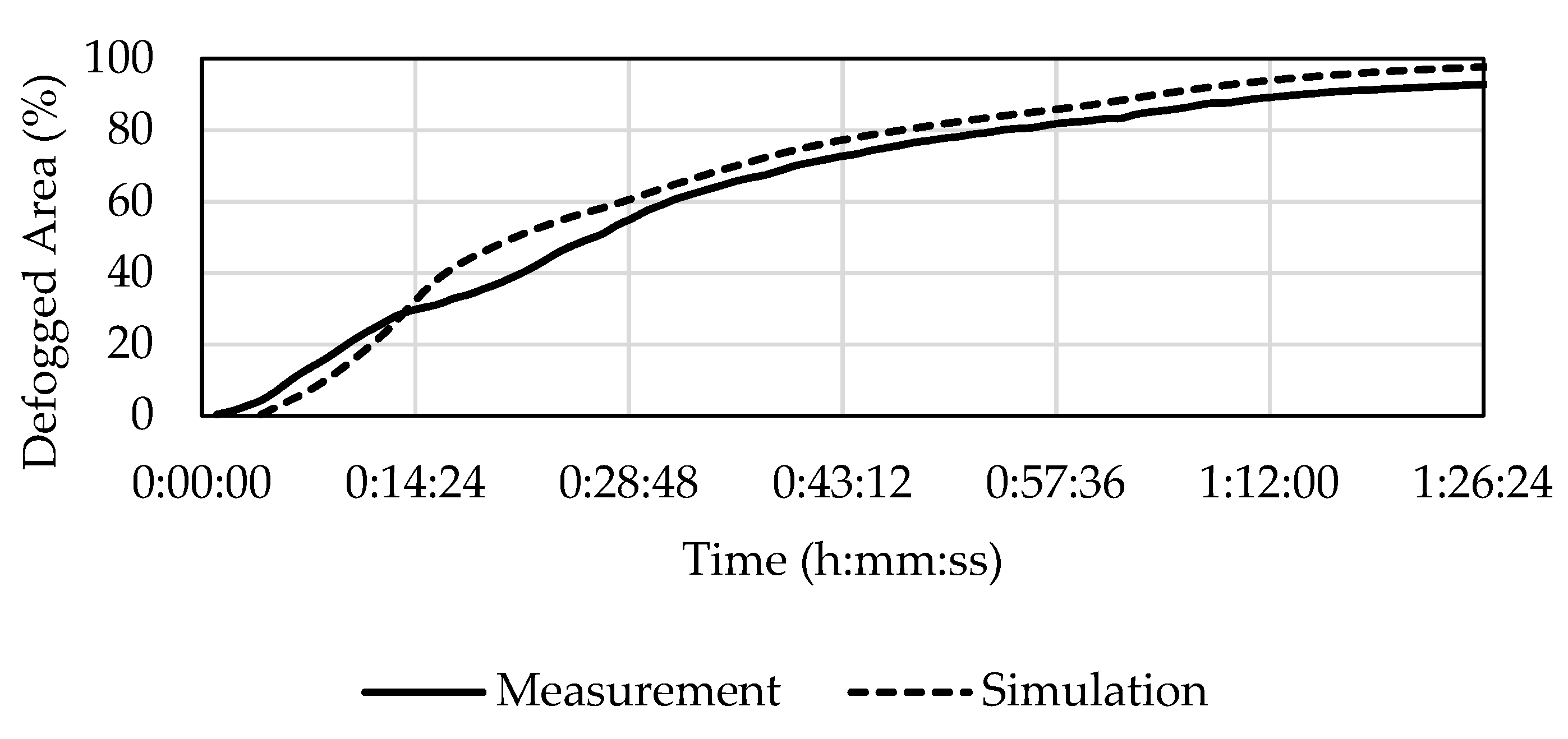
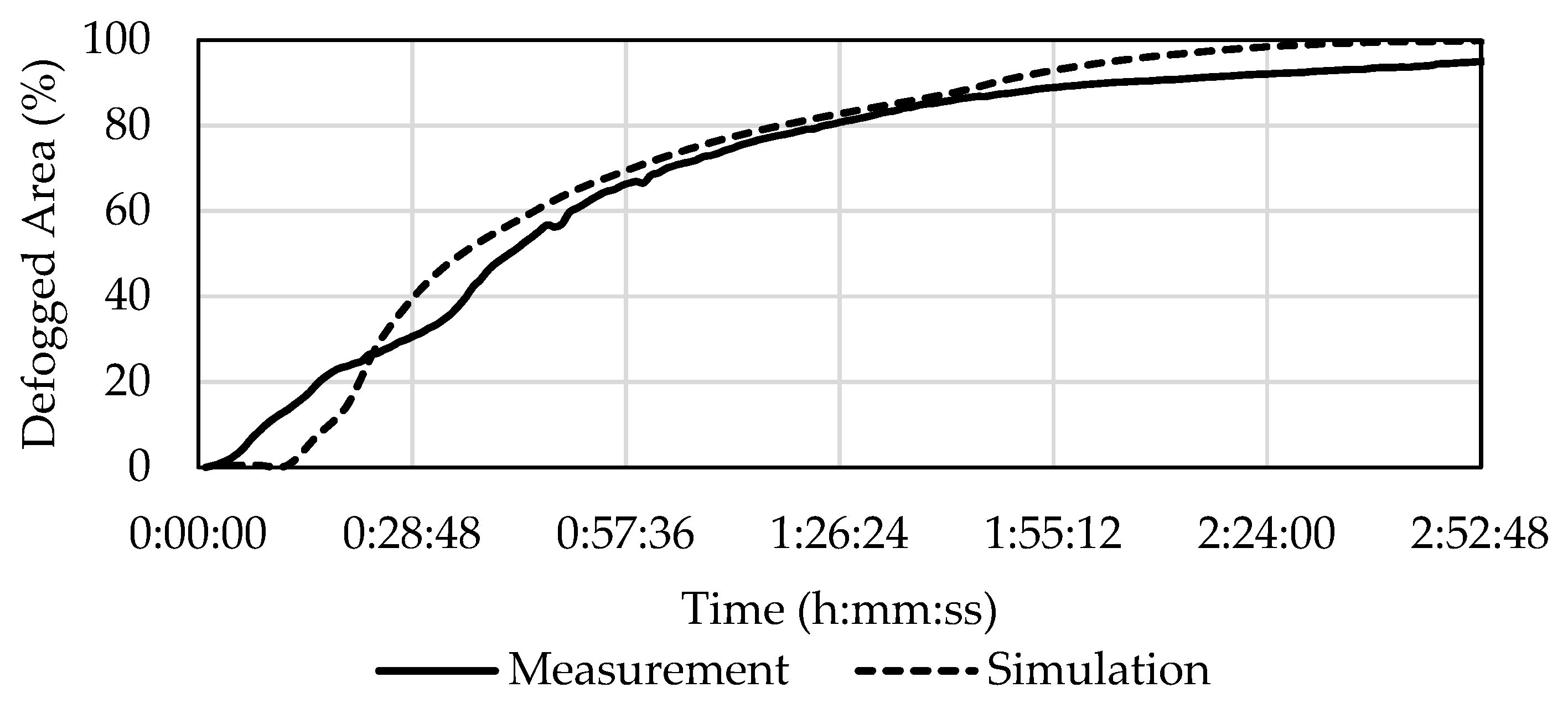
In experiment C1, which had the lowest amount of evaporated water (1 mL), a good match with the numerical simulation was found. According to

Table 6. Time comparison of the defogging duration in C1.

	50% Defogged (h:mm:ss)	80% Defogged (h:mm:ss)
Experiment	0:26:00	0:48:00
Simulation	0:21:14	0:47:10
Offset	0:04:46	0:00:50

, the defogging curves reached 50% of the defogged area in 26 min in the experiment and in 21 min and 14 s in the simulation (i.e., 18% sooner). In the experiment it took 48 min to reach 80% of the defogged area in comparison to 47 min and 10 s for the simulation (i.e., 2% sooner).

The defogging curves in Figure 9 have almost the same behavior after the initial 29 min with a slight offset which represents approximately 3.5%, which is equal to the amount of the unevaluable area from image processing.

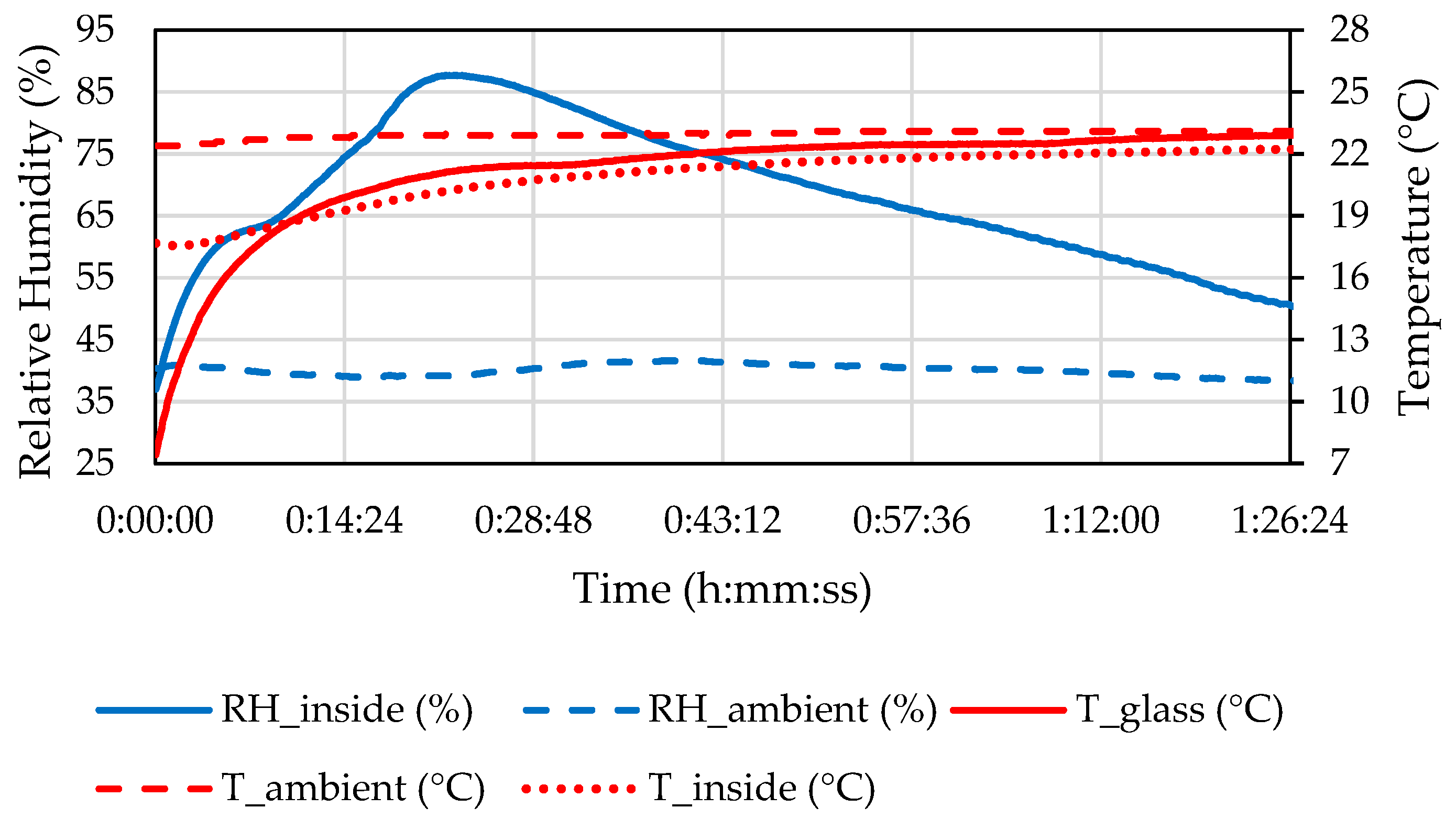
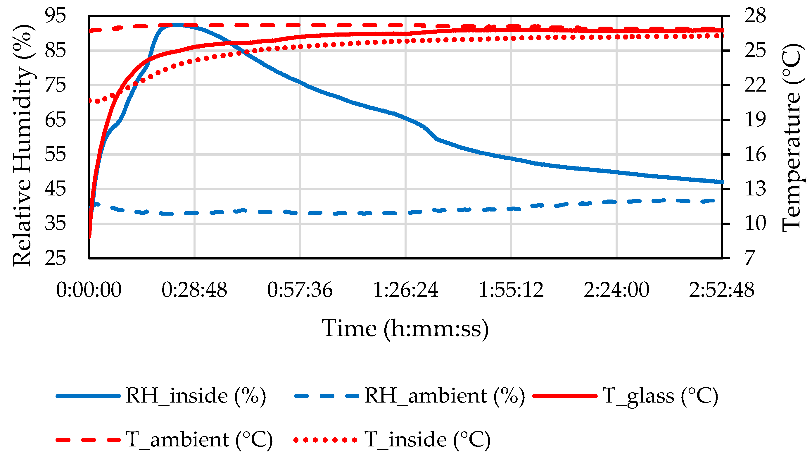
The measured properties of the ambient air and the air inside the headlamp during the defogging in C1 are shown in Figure 10.

Table 7. Visual comparison of C1 results (red—fogged, green—defogged, blue—unevaluable).

Experiment	Simulation
Beginning of defogging
12 min from the beginning of defogging
24 min from the beginning of defogging
36 min from the beginning of defogging
1 h from the beginning of defogging
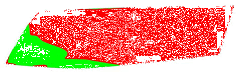
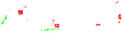
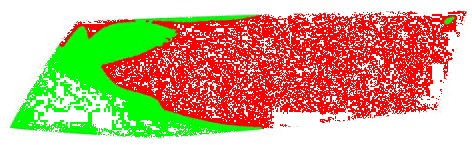
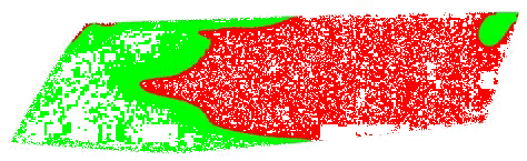
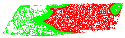
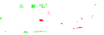
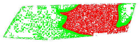
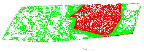
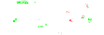
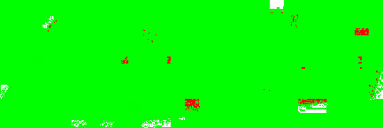
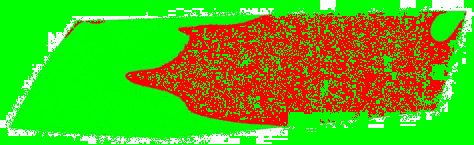
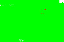
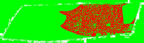
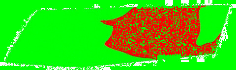
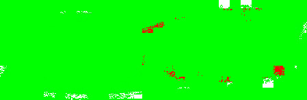
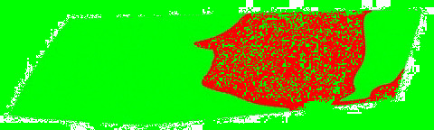
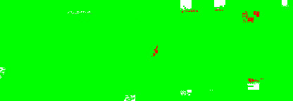
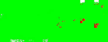
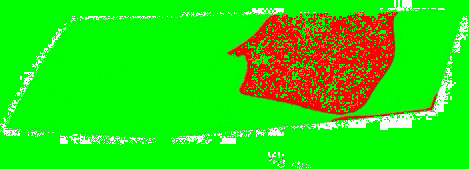
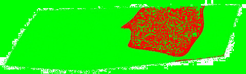
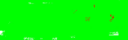
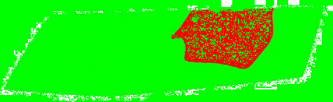
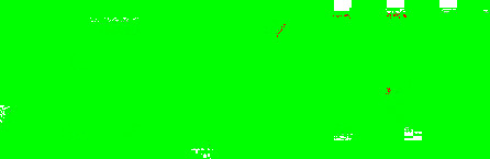
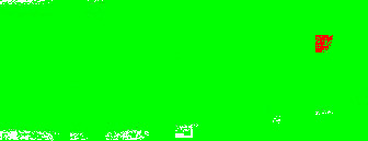
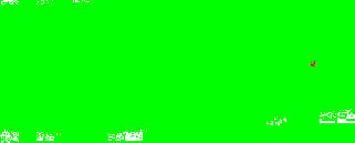
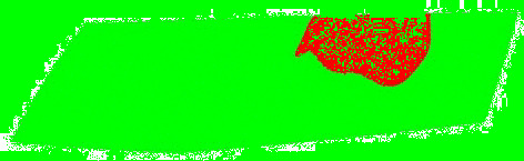
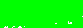
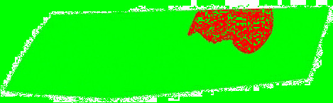
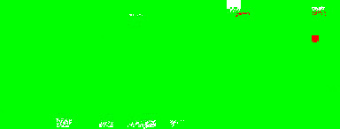
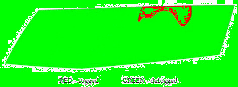
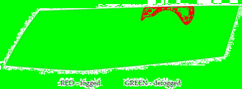
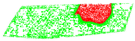
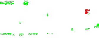
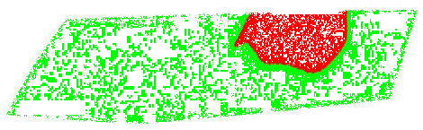
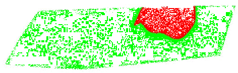
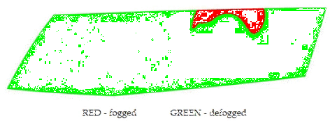
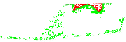
End of defogging

presents processed laboratory experiment images with their numerical simulation counterparts in the case of C1. The red area represents the fogged area, the green area represents the area which has already been defogged, and in the case of processed imagery, the blue areas are the parts of the glass which the program was unable to evaluate. These areas were caused by reflected light or insufficient fogging of the glass’ borders.

From visual comparison of these results, it is possible to conclude that in the case of experiment C1 and its corresponding simulation, the difference in the defogging process was small. The top-right area was defogged last in both cases. As this was caused by the position of the humidifier, the most heavily fogged area was situated near it. Some differences can be found here. In the case of the experiment C1 the condensate stayed in the left part of the glass longer and disappeared slowly from the bottom up. In the case of the simulation, the condensate disappeared from the borders to the area in front of the humidifier.

5.2. Comparison of Results C1.5—1.5 mL of Evaporated Water

The results were very similar in experiment C1.5 (1.5 mL of evaporated water). The simulation only differed significantly from the experiment in the first 19 min, as can be seen in Figure 11. The image processing was unable to evaluate 3.5% of the front glass area, which again explains the difference between the experiment and the simulation. According to

Table 8. Time comparison of defogging duration in C1.5.

	50% Defogged (h:mm:ss)	80% Defogged (h:mm:ss)
Experiment	0:31:00	1:08:00
Simulation	0:30:00	1:06:00
Offset	0:01:00	0:02:00

, 50% defogging took 31 min for the experiment and 30 min in the simulation (i.e., 3% quicker). In the experiment it took 1 h and 8 min to reach 80% defogged area, while in the simulation it took 1 h and 6 min (i.e., 3% quicker).

Measured properties of the ambient air and the air inside the headlamp during the defogging in C1.5 are shown in Figure 12.

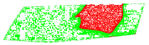
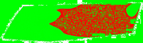
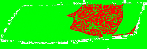
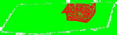
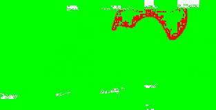
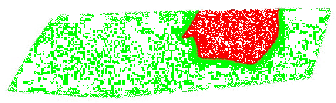
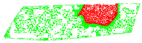
The processed laboratory experiment images with their numerical simulation counterparts for C1.5 are displayed in

Table 9. Visual comparison of C1.5 results (red—fogged, green—defogged, blue—unevaluable).

Experiment	Simulation
Beginning of defogging
28 min from the beginning of defogging
44 min from the beginning of defogging
1 h and 8 min from the beginning of defogging
1 h and 36 min from the beginning of defogging
End of defogging

. This visual comparison also shows a good match between the experiment and the simulation. The main difference is that in the case of the simulation the area fogged for the longest time was in front of the humidifier but according to the experiment almost the entire upper border took a long time to defog.

5.3. Comparison of Results C2—2 mL of Evaporated Water

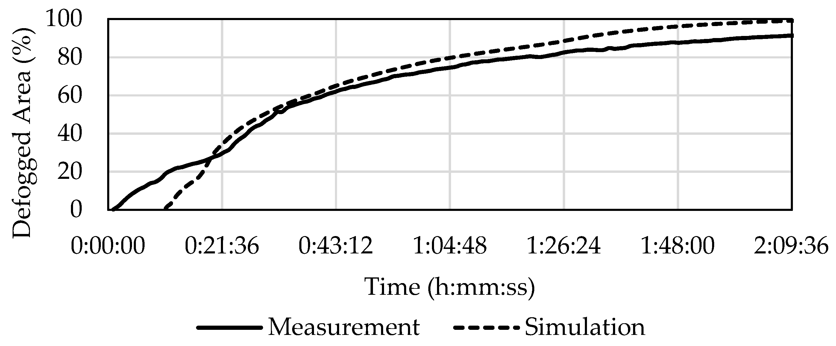
The difference between the experiment C2 and its simulation was similar to the difference seen in C1.5. The results differed significantly for the first 30 min of defogging, but after that there was a slight difference caused by the unprocessable area. In the experiment, 50% defogging occurred after 41 min and in the simulation it occurred after 35 min and 33 s (i.e., 13% quicker). According to

Table 10. Time comparison of defogging duration in case C2.

	50% Defogged (h:mm:ss)	80% Defogged (h:mm:ss)
Experiment	0:41:00	1:24:00
Simulation	0:35:33	1:18:34
Offset	0:05:27	0:05:34

the experiment reached 80% defogged area in 1 h and 24 min, whereas for the simulation 80% defogging was reached in 1 h, 18 min, and 34 s (about 6.5% faster).

The development of defogging over time is displayed in Figure 13.

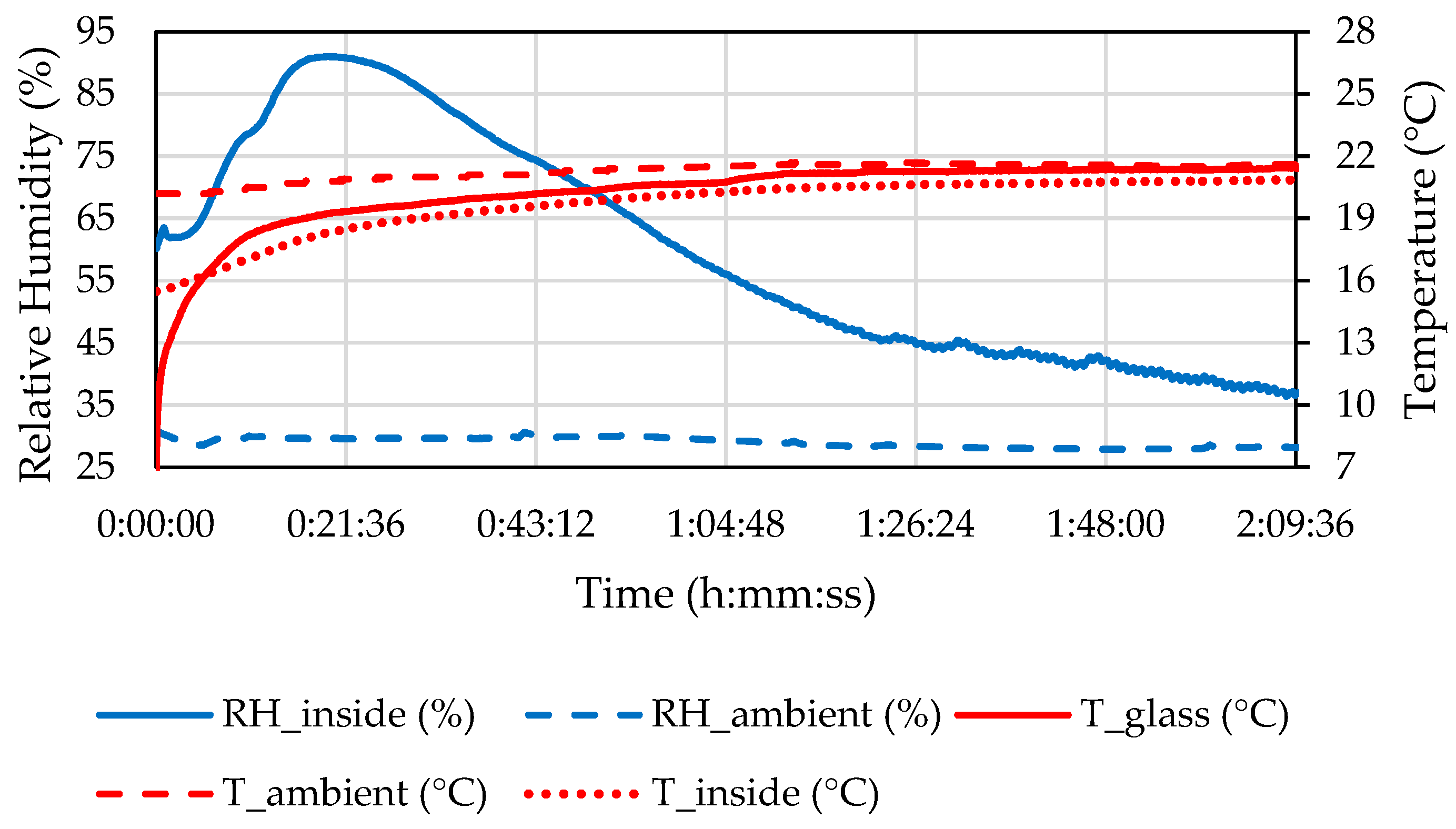
The measured properties of the ambient air and the air inside the headlamp in C2 are shown in Figure 14.

Table 11. Visual comparison of C2 results (red—fogged, green—defogged, blue—unevaluable).

Experiment	Simulation
Beginning of defogging
28 min from the beginning of defogging
44 min from the beginning of defogging
1 h and 8 min from the beginning of defogging
1 h and 36 min from the beginning of defogging
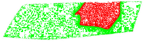
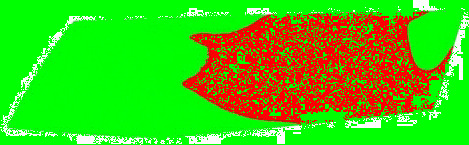
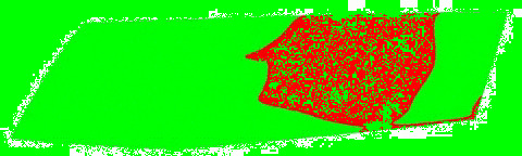
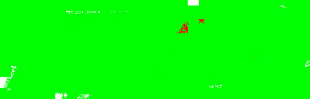
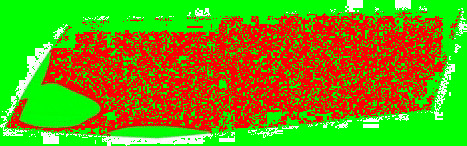
End of defogging

visually presents the differences in the C2 experiment and its corresponding simulation. We can see similar differences in the case of the C2 experiment and its simulation as in the case of C1.5. The condensate disappeared around the borders of the glass and in the area where the humidifier was situated, and in the experiment the upper border took far longer to defog. We can observe that in the case of the simulation the condensate stayed in the bottom-left corner longer than in the experiment.

6. Conclusions

We conducted three numerical simulations of headlamp defogging with different amounts of condensed water on the front glass of a headlamp. These simulations copied the laboratory experiments of a new approach in headlamp fogging–defogging testing, developed in the Heat Transfer and Fluid Flow Laboratory of Brno University of Technology, Faculty of Mechanical Engineering.

The simulations were conducted in the commercially available software ANSYS Fluent. Eulerian wall film was chosen as a numerical model for the prediction of condensation and evaporation. We compared the time needed to defog the front glass area between the experiments and the simulations.

The visual results from simulations showed the same progression of defogging, beginning on the right-hand side of the glass and in the upper-left corner, ending near the humidifier. Only the total time changes depending on the amount of condensed water. We could see a similar situation in the experiments, the main difference being that the upper glass border remained fogged almost until the end.

The simulations showed a very good match to the real experiments, with a larger difference in the initial parts. This can be explained by a fast heating of the front glass and steep rise of the internal humidity (as shown in Figure 10, Figure 12, and Figure 14). EWF seemed to be unable to simulate this quick change accurately. For the rest of the simulations, all three scenarios produced results very close to the experiments with only a slight difference of approximately 3%, caused by small unprocessable areas in the experiment photos. Other differences in results may have been caused by the numerical model used, which is less precise than for example the volume of fluid method but requires lower computational power. Boundary conditions were chosen based on the experiments, but some inaccuracy could create further differences.

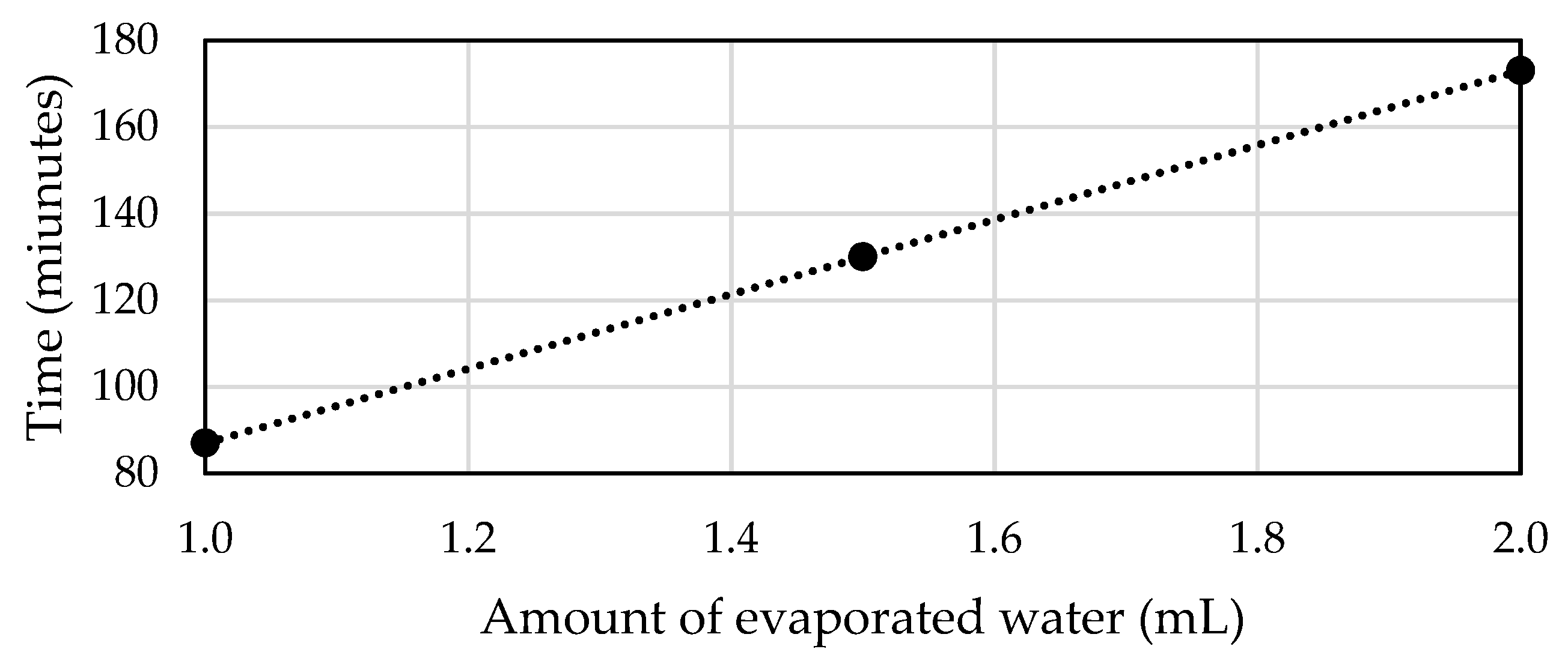
With regard to these slight differences, we can assume that the developed simulations could be further used to estimate defogging development over time and compare the whole process with different pressure settings on the ventilation holes instead of numerous experiments. Only a few of the best configurations, according to the simulations, can be further verified by real testing.

Table 12. Comparison of results achieved from all three experiments.

	C1	C1.5	C2
Amount of evaporated water (mL)	1	1.5	2
Total defogging time (h:mm)	1:27	2:10	2:53
Ambient temperature (°C)	23.1	21.0	27.0
Ambient humidity (%)	38.9	29.5	41.1

presents a complete comparison of the experiments. We can clearly observe that the total amount of defogging time was linearly dependent on the amount of condensed water.

From these results we could obtain a trend line and its equation, as seen in Figure 15, which can serve as an estimation of defogging time for other amounts of evaporated water.

The trend line equation is:

$$t_{def}=86·V_w+1,$$

(11)

where $t_{def}$ is the defogging time and $V_w$ is the amount of evaporated water.

7. Patents

GUZEJ, M.; HORSKÝ, J.; Vysoké učení technické v Brně, Brno, CZ: Zařízení ke zvlhčení vnitřního prostoru světlometu. 305743, patent. (2016)

References

- Kouloh, H.; Geissler, U.; Weber, D.; Mueller, A. Active Moisture Removal Puts Headlamp Condensation Protection on a New Level. In SIA VISION 2018; Technical Paper; Société des ingénieurs de l’automobile: Paris, France, 2018; pp. 103–109. [Google Scholar]
- Tseng, K.-W.; Chen, T.-H.; Chen, S.-J.; Su, Y.-D.; Wang, H.-C.; Feng, S.-W.; Ye, Z.; Tu, K.-H. Laser Headlamp with a Tunable Light Field. Energies 2019, 12, 707. [Google Scholar] [CrossRef]
- Sun, Y.S.; Emery, A.F. Effects of wall conduction, internal heat sources and an internal baffle on natural convection heat transfer in a rectangular enclosure. Int. J. Heat Mass Transf. 1997, 40, 915–929. [Google Scholar] [CrossRef]
- Barozzi, G.; Corticelli, M. Natural convection in cavities containing internal sources. Heat Mass Transf. 2000, 36, 473–480. [Google Scholar] [CrossRef]
- Jue, T.C. Analysis of thermal convection in a fluid-saturated porous cavity with internal heat generation. Heat Mass Transf. 2003, 40, 83–89. [Google Scholar] [CrossRef]
- Groce, G.; D’Agaro, P.; Mattiello, F.; De Angelis, A. A Numerical Procedure for Defogging Process Simulation in Automotive Industry. In Proceedings of the International Conference on Heat and Mass Transfer, Corfu, Greece, 17–19 August 2004; pp. 17–19. [Google Scholar]
- Croce, G.; D’Agaro, P.; De Angelis, A.; Mattiello, F. Numerical simulation of windshield defogging process. Proc. Inst. Mech. Eng. Part D J. Automob. Eng. 2007, 221, 1241–1250. [Google Scholar] [CrossRef]
- Moore, W.I.; Powers, C.R. Temperature Predictions for Automotive Headlamps Using a Coupled Specular Radiation and Natural Convection Model; SAE Technical Paper; SAE International: Warrendale, PA, USA, 1999. [Google Scholar] [CrossRef]
- Singh, R.; Kuzhikkali, R.; Shet, N.; Natarajan, S.; Kizhedath, G.; Arumugam, M. Automotive LED Headlamp Defogging: Experimental and Numerical Investigation; SAE Technical Paper; SAE International: Warrendale, PA, USA, 2016. [Google Scholar] [CrossRef]
- Deponti, A.; Damiani, F.; Brugati, L.; Bucchieri, L.; Zattoni, S. Modelling of condensate formation and disposal inside an automotive headlamp. In Proceedings of the 4th European Automotive Simulation Conference, Munich, Germany, 6–7 July 2009. [Google Scholar]
- Engineering ToolBox. 2001. Available online: https://www.engineeringtoolbox (accessed on 15 May 2019).
- Incropera, F.; Dewitt, D. Fundamentals of Heat and Mass Transfer, 6th ed.; John Wiley: Hoboken, NJ, USA, 2007; ISBN 978-047-1457-282. [Google Scholar]
- Curcio, J.A. Adsorption and Condensation of Water on Mirror and Lens Surfaces; U.S. Naval Research Lab.: Washington, DC, USA, 1976. [Google Scholar]
Figure 1.
Schematic of the test rig (1: pressurized air; 2: regulators; 3: humidifier; 4: headlamp; 5: camera).
Figure 2.
Testing rig used for fogging/defogging (1: pressurized air; 2: regulators; 3: humidifier; 4: headlamp).
Figure 3.
Main dimensions of the headlamp.
Figure 4.
Geometric model used for the numerical simulations. (left) Position of the humidifier; (right) positions of the vent holes (1−4: inlets; 5: outlet).
Figure 5.
Cross section of the domain. (left) simulation of fogging (preparative stage); (right) simulation of defogging (evaluated stage).
Figure 6.
Cross section of the mesh with detailed view of the front glass and humidifier areas.
Figure 7.
Evaporation of thin water film on the front glass.
Figure 8.
Velocity distribution inside the headlamp in case C2—cross section through the humidifier. (left) Simulation of fogging (preparative stage—20 min since the beginning of humidification); (right) simulation of defogging (evaluated stage—30 min since the beginning of defogging).
Figure 9.
Development of defogging in C1 according to the experiment and the simulation.
Figure 10.
Temperature and relative humidity (RH) of the ambient air and inside the headlamp and the temperature of the front glass during the C1 defogging phase.
Figure 11.
Development of defogging in C1.5 according to the experiment and the simulation.
Figure 12.
Temperature and relative humidity of the ambient air, air inside the headlamp, and temperature of the front glass during the C1.5 defogging phase.
Figure 13.
Development of defogging in C2 according to the experiment and the simulation.
Figure 14.
Temperature and relative humidity of the ambient air and inside the headlamp and temperature of the front glass during the C2 defogging phase.
Figure 15.
Trend line from defogging time of all three experiments.