Recognition and Classification of Incipient Cable Failures Based on Variational Mode Decomposition and a Convolutional Neural Network

Abstract

To avoid power supply hazards caused by cable failures, this paper presents an approach of incipient cable failure recognition and classification based on variational mode decomposition (VMD) and a convolutional neural network (CNN). By using VMD, the original current signal is decomposed into seven modes with different center frequencies. Then, 42 features are extracted for the seven modes and used to construct a feature vector as input of the CNN to classify incipient cable failure through deep learning. Compared with using the original signals directly as the CNN input, the proposed approach is more efficient and robust. Experiments on different classifiers, namely, the decision tree (DT), K-nearest neighbor (KNN), BP neural network (BP) and support vector machine (SVM), and show that the CNN outperforms the other classifiers in terms of accuracy.

1. Introduction

The development process of cable failure is usually divided into three stages: the partial discharge period, incipient failure period and permanent failure period [1]. Due to defect formation, corrosion or aging of the insulating layer, a series of partial discharge pulses first appear in the cable, forming electrical or water branches. With further deterioration, these branches would evolve into incipient failures accompanied by arcing. Incipient failures advance progressively after the first occurrence to the point of irreversible permanent failure [2]. The occurrence of incipient cable failure (also known as self-cleaning failure) is uncertain, and the current, which is very small when failure occurs, is typically not sufficient to trigger the safety protection of traditional overcurrent detection devices [3,4]. At the same time, because of the similarity with other disturbances, e.g., overcurrents caused by transformer inrush current, constant impedance and capacitor switching failures, it is relatively difficult to recognize incipient cable failures accurately. Therefore, it is of great significance for the stable operation of power grid to achieve an approach that can effectively recognize and classify incipient cable failures and to complete cable maintenance in time before incipient failures become permanent failures.

Due to the uncertainty of the transmission environment and the effects of noise, the actual cable signals usually contain a large amount of interference information. Especially under high noise conditions, the features of incipient cable failure are so weak that it is difficult to directly recognize them. Therefore, it is necessary to perform signal preprocessing before classification. At present, many researchers have proposed different approaches for the recognition and classification of cable failures. The recognition methods are mainly divided into fault detection methods based on hardware design [5,6,7,8] and feature extraction based on time-frequency analysis [9,10,11,12,13,14]. In [5], a hardware relay implementation in power systems is presented, which by using a proposed syntactic pattern [6], reads each peak of the examined signals to detect existing faults. The effectiveness of the proposed relay is determined by the user setting suitable thresholds. In [7], the waveform is monitored for alarming distortion by using the proposed amplitude tracking algorithm in a field programmable gate array (FPGA). In [8], Romano et al. presented an antenna sensor to measure partial discharge. The results show that the instrument can diagnose the health of the insulation system quickly and accurately. Obviously, fault detection based on hardware design is fast and real-time, but it also depends on hardware algorithms, and the threshold setting and portability of the devices must be considered.

Feature extraction methods based on time-frequency analysis include short-time Fourier transform (STFT) [9], wavelet transform (WT) [10], and empirical mode decomposition (EMD) [11]. In [12], an arc fault recognition systems that combine STFT with hardware devices is described; the system checks whether the harmonic components in the frequency domain exceed a threshold value that is set according to limited testing loads in the lab. The STFT overcomes the shortcoming of frequency domain time information loss of the Fourier transform, and realizes local time-frequency analysis of the signal. However, the size of the window function cannot change with frequency, which is not conducive to analyzing time-varying signals. In [13], Sidhu et al. decomposed the original current signals via WT, and the overcurrent disturbance was initially recognized by using the energy and root mean square value at the fault location; then, incipient cable failure was identified by adjusting the thresholds. Chao et al. [14] detected incipient cable failure based on the overcurrents and the WT modulus maximum of the sum of single-end sheath currents. When the magnitude of the sum of sheath currents exceeds the theoretical value, an overcurrent condition can be diagnosed. Then, one can set the threshold based on the normal signal for the WT modulus maxima of the sum of sheath currents to determine whether the overcurrents are generated by incipient failure. WT inherits and develops the idea of STFT localization, and it overcomes the shortcomings of window fixation. However, its decomposition results depend too much on the choice of wavelet basis. In [15], the instantaneous frequency component of the partial discharge signal of the cable joint was obtained via EMD, and then the 3D (time-frequency-energy) Hilbert spectrum was calculated. Finally, partial discharge types were evaluated by using a neural network. EMD not only breaks through the limitations of FT, but also does not have the problem of preselecting wavelet basis function such as the wavelet transform. It has good time-frequency resolution and adaptability. However, this algorithm lacks a mathematical foundation. In particular, modal aliasing problems are easily generated during the decomposition process.

In this paper, a feature extraction method based on time-frequency analysis of variational mode decomposition (VMD) and mathematical statistics is used. VMD was proposed by Dragomiretskiy et al. in 2014 [16]; it is a complete nonrecursive adaptive and quasi-orthogonal signal decomposition method that decomposes multicomponent nonstationary signal into several components with limited bandwidth. The essence of VMD is that multiple sets of Wiener filters are updated directly in the Fourier domain; thus, VMD has a more solid theoretical basis and robustness than EMD [17,18]. At the same time, 42 features are extracted by the method of mathematical statistics, which solves the feature selection problem and improves the calculation efficiency.

Fault classification methods can be categorized into machine learning algorithms and deep learning algorithms. Machine learning algorithms, including decision tree (DT), support vector machine (SVM), K-nearest neighbor (KNN), and artificial neural network (ANN), have been widely used in power systems [19,20,21,22,23]. Recently, researchers have conducted studies of traditional algorithms for different problems and further improved the classification accuracy [24,25,26]. However, these classifiers still have some defects, such as a weak correlation between data, a tendency to overfit and a limited capacity for the real-time processing of large data. A deep learning model is a network structure that updates the parameters of multiple hidden layers via a gradient descent algorithm, which overcomes the shortcomings of machine learning algorithms and solves the problems of data utilization, gradient diffusion and trapping in local optima [27,28]. The representative structures are the deep belief network (DBN) [29], the recurrent neural network (RNN) [30,31] and the convolutional neural network (CNN) [32]. The DBN algorithm can reflect the similarity of the same type of data itself, but since its generation model does not care about the optimal classification surface, the classification accuracy is usually not as high as that of the discrimination model. The RNN has time memory ability through recursive method, but it requires more training parameters and is prone to gradient dissipation or gradient explosion.

This paper uses the CNN algorithm; as one of the deep learning models, its multilevel structure of local perception and value sharing can accommodate high-dimensional data more accurately and quickly. Due to the characteristics of self-learning, especially the results are stable in the field of image and signal recognition, and there is no additional feature engineering requirement [33].

This paper presents a new approach for incipient cable failure recognition and classification based on VMD feature extraction and CNN classification (Figure 1). Via VMD, features of each decomposed mode for the original signal are extracted, and feature vector is input into the CNN to recognize incipient cable failure. The paper is organized as follows: in Section 2, the VMD principle, mathematical model and CNN algorithm are described. In Section 3, experimental data are generated by constructing a model of incipient cable failure and overcurrent interference in PSCARD/EMTDC. Next, the complete experimental results are shown. Compared with traditional machine learning algorithms (DT, KNN, BP, and SVM), the proposed approach not only can recognize incipient cable failure state well but also has good noise immunity. In Section 4, the produced results are commented and the limitations of the research are expounded. In the last section, the conclusions are summarized.

2. Methods

2.1. VMD

VMD is used to decompose the nonstationary cable signal x(t) into a number of subcomponents (known as modes), with each mode having a finite bandwidth corresponding to the center frequency. Thus, VMD aims to minimize the sum of the bandwidth estimate of each mode. To adaptively extract modes and their central frequencies, an optimization problem is constructed as follows:

First, let x(t) be predecomposed into K modes, denoted as $u_k$ $\left(k=1,\cdots ,K\right)$, i.e., ${\displaystyle \sum _{k=1}^K{u}_k=x\left(t\right)}$. To acquire the unilateral frequency spectrum, the associated analysis signal of u_k is formed by using the Hilbert transform as follows:

$$\left[\delta \left(t\right)+\frac{j}{\pi t}\right]\ast u_k\left(t\right),$$

(1)

where δ(t) is the Dirac delta function, j is an imaginary number, and * is the convolutional operation.

Then, for each mode $u_k$, its frequency spectrum is modulated to the baseband through multiplying the corresponding analysis signal by the exponential $e^{-j{\omega }_{k}t}$, where ${\omega }_k$ is the center frequency of $u_k$.

Next, to adaptively extract $u_k$ and ${\omega }_k$, by using the L²-norm of the demodulated signal’s gradient, the constrained variational optimization problem is constructed as follows:

$$\{\begin{array}{l}\underset{\left\{u_k\right\},\left\{w_k\right\}}{\min }\left\{{\displaystyle \sum _{k=1}^K{\Vert {\partial }_t\left[(\delta (t)+\frac{j}{\pi t})*u_k(t)\right]e^{-j{\omega }_{k}t}\Vert }_2^2}\right\}\\ s.t.{\displaystyle \sum _{k=1}^K{u}_k=x\left(t\right)(k=1,\cdots ,K)}\end{array},$$

(2)

where ${\partial }_t(\cdot )$ is the partial derivative and ${\Vert \cdot \Vert }_2$ is the L²-norm.

Finally, to solve for $u_k$ and ${\omega }_k$ in (1), by using the augmented Lagrange multiplier method [34], the constrained variational problem (2) is transformed into the following unconstrained variational problem:

$$\begin{array}{c}L(\{u_k\},\{{\omega }_k\},\lambda )=\alpha {\displaystyle \sum _{k=1}^K{\Vert {\partial }_t\left[(\delta (t)+\frac{j}{\pi t})\ast u_k(t)\right]e^{-j{\omega }_{k}t}\Vert }_2^2}+{\Vert x(t)-{\displaystyle \sum _{k=1}^K{u}_k}(t)\Vert }_2^2+\\ \langle \lambda (t),x(t)-{\displaystyle \sum _{k=1}^K{u}_k}(t)\rangle \end{array}$$

(3)

where λ is Lagrange multiplier and α is the parameter to balance variational term (the first term) and data-fidelity constraint term (the second term), so as to impart good reconstruction accuracy to the signal.

Then, $u_k$, ${\omega }_k$ and λ in (2) are iteratively and alternately updated by using the alternating direction multiplier method (ADMM) in the Fourier domain [15]. In the nth iteration, $u_k^{n+1}$ and ${\omega }_k^{n+1}$ are calculated in the Fourier domain as follows:

$${\widehat{u}}_k^{n+1}(\omega )=\frac{\widehat{x}(\omega )-{\displaystyle \sum _{i\ne k}^K{\widehat{u}}_i(\omega )}+\frac{\widehat{\lambda }(\omega )}{2}}{1+2\alpha {(\omega -{\omega }_k)}^2},$$

(4)

and:

$${\omega }_k^{n+1}=\frac{{\displaystyle {\int }_0^{\infty }\omega {\left|{\widehat{u}}_k(\omega )\right|}^{2}d\omega }}{{\displaystyle {\int }_0^{\infty }{\left|{\widehat{u}}_k(\omega )\right|}^{2}d\omega }},$$

(5)

respectively. The Lagrange multiplier λ is updated as follows:

$${\widehat{\lambda }}^{n+1}\left(\omega \right)={\widehat{\lambda }}^n\left(\omega \right)+\tau \left[\widehat{x}(\omega )-{\displaystyle \sum _k{\widehat{u}}_k^{n+1}\left(\omega \right)}\right].$$

(6)

where τ is the time step of the dual ascent. Once ${{{\displaystyle \sum _k\Vert {\widehat{u}}_k^{n+1}-{\widehat{u}}_k^n\Vert }}_2^2/\Vert {\widehat{u}}_k^n\Vert }_2^2<\epsilon \left(\epsilon >0\right)$ is satisfied, the iteration process is over, and ${\omega }_k$ is obtained. Furthermore, the mode $u_k$ in the time domain is obtained as the real part of the inverse Fourier transform of ${\widehat{u}}_k$.

2.2. Feature Extraction

VMD decomposes the input signal into multifrequency signals, which is helpful for effectively distinguishing incipient cable failure from that of other disturbances. Obviously, the decomposed multilayer signals have more data. If input them into the CNN for classification directly would increase the difficulty of selecting the network parameters and the training time be too long. Thus, to achieve the aim of efficiently training the CNN, features extracted from decomposed VMD modes are used as inputs of the CNN below. For each VMD mode with N sample points, denoted as $u_k\left[n\right]$ $\left(1\le n\le N\right)$, six features are extracted as follows:

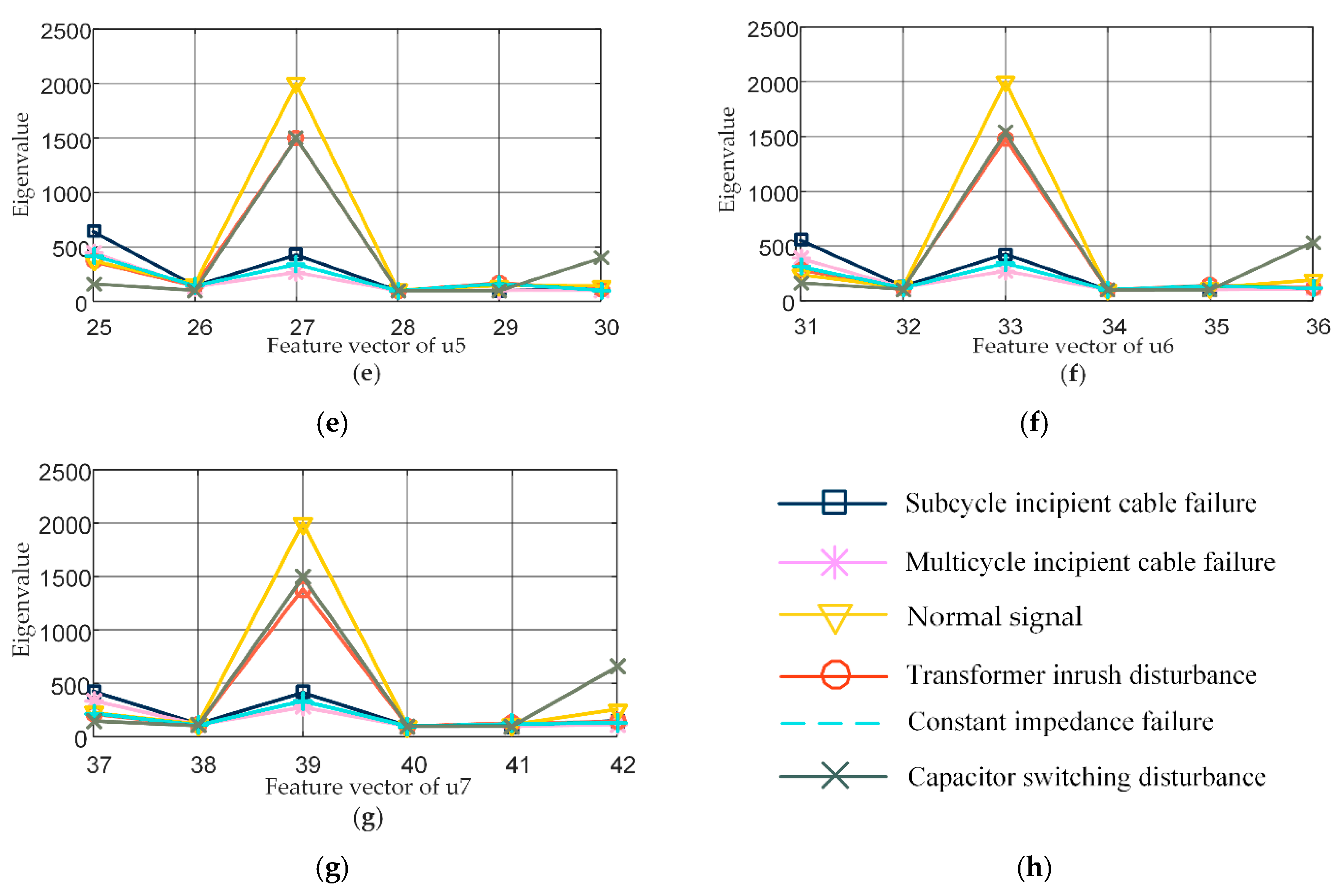
• F1: F1 represents the peak-to-peak value, i.e., the range of signal amplitude variation. An observation of six types of signals indicates that F1 of multicycle cable failure is several times that of other signals. Therefore, this feature plays a key role in distinguishing between multicycle cable failure from the range of amplitudes of different signals. For the k-th mode, F1 is given by:

  $$F{1}_k=max\left(u_k\left[n\right]\right)-min\left(u_k\left[n\right]\right).$$

  (7)
• F2: This feature is the root mean square (RMS), which represents the effective value of the periodic signal. Because the RMS is the squared average calculated over one cycle, the feature helps to separate all multicycle failure signals from other types. Hence, F2 is an important reference in the recognition of multicycle cable failure, normal signals, transformer inrush disturbance and constant impedance failure. For the kth mode, F2 is given by:

  $$F{2}_k=\sqrt{\frac{1}{N}{\displaystyle {\sum }_n{u}_k^2\left[n\right]}}.$$

  (8)
• F3: The feature F3 represents the number of zero crossings, which is used to identify the oscillatory characteristics and noise of the stationary signal for each mode. For the kth mode, F3 is computed as follows:

  $$F{3}_k={\displaystyle \sum _n\left|\mathrm{sgn}\left(u_k\left[n\right]\right)-\mathrm{sgn}\left(u_k\left[n-1\right]\right)\right|}/2.$$

  (9)
  Here, $\mathrm{sgn}(\cdot )$ is a symbolic function. Taking into account the duration of different nonstationary signals at the zero position, F3 reflects the state of the waveform, where the signal crosses zero for each mode, which is helpful to distinguish the overcurrent disturbance, normal signal and noise.
• F4: The mode relative energy ratio represents the contribution of the energy of each mode to the total energy of the original signal. For the kth mode, this ratio is denoted as:

  $$F{4}_k=\frac{{\displaystyle {\sum }_n{u}_k^2\left[n\right]}}{{\displaystyle {\sum }_k{\displaystyle {\sum }_n{u}_k^2\left[n\right]}}}.$$

  (10)
  The main energy of different signals is distributed over different decomposition modes, e.g., the energy of the normal signals is mainly distributed over the first one decomposition mode, and the latter modes contain only DC components. According to this feature, incipient cable failure, normal signals and overcurrent disturbance can be distinguished accurately.
  F5: The instantaneous amplitude envelope of each mode is used to distinguish between short- and long-duration variations (such as subcycle failure, transformer inrush disturbance and constant impedance failure). For the k-th mode, F5 is defined using a sliding window of length s as follows:

  $$F{5}_k=\sqrt{\frac{1}{s}{\displaystyle \sum _{n=m}^{m+s-1}{u}_k^2\left[n\right]}}.$$

  (11)
  Here, $m=1,2\cdots (N-s+1)$ represents the number of sliding windows.
• F6: The center frequency (${\omega }_K$) is selected as the sixth feature. Since the VMD process is implemented in the frequency domain, this condition eliminates the need for additional calculation of the frequency domain information of each mode. F6 is used to distinguish the DC component, fundamental frequency, and oscillation of different modes.

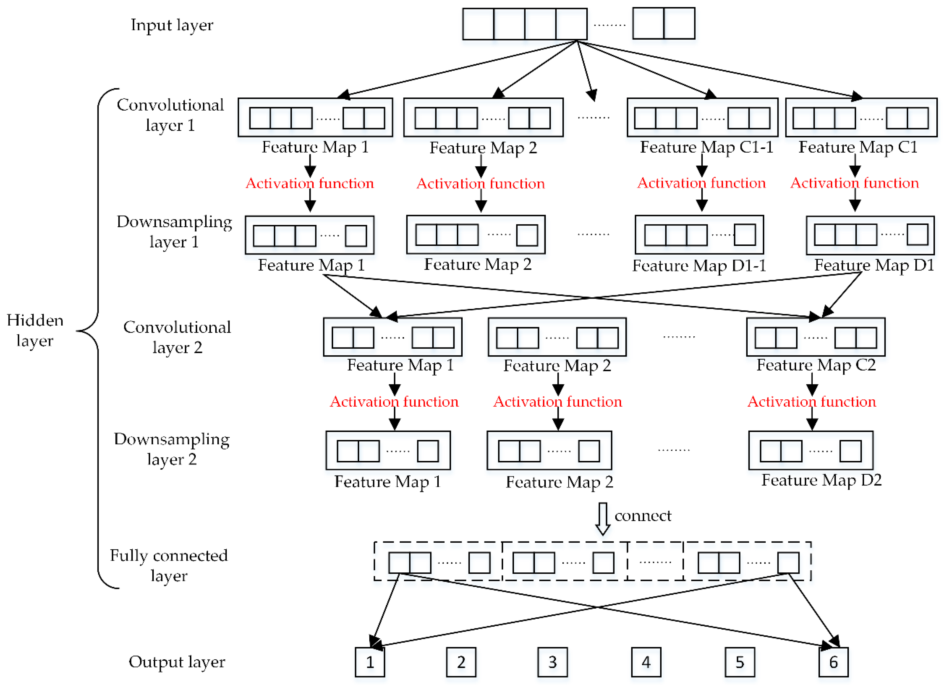
Based on the abovementioned features, the feature vector for the k-th mode can be obtained as follows:

$$F{V}_k=\left[F{1}_k,F{2}_k,F{3}_k,F{4}_k,F{5}_k,F{6}_k\right].$$

(12)

In summary, assuming that the original signal is decomposed into K modes via VMD, a $1\times 6K$ feature vector F can be composed as follows:

$$F=\left[\begin{array}{cccc}F{V}_1& F{V}_2& \cdots & F{V}_K\end{array}\right]=\left[\begin{array}{cccccccc}F{1}_1& \cdots & F{6}_1& F{1}_2& \cdots & F{6}_2& \cdots \cdots & \begin{array}{cc}\begin{array}{cc}F{6}_K& \cdots \end{array}& F{6}_K\end{array}\end{array}\right].$$

(13)

Then, F is input to the CNN as all feature information of the original signal.

2.3. CNN

The CNN is constructed by analogy to animal visual perception. Its structure of multilayer perceptron can effectively reduce preprocessing, and it can also analyze high-dimensional data. Hence, the CNN has exhibited excellent performance in the field of image and video recognition and signal processing.

The CNN consists of an input layer, an output layer and a hidden layer. As the most important part of the whole network, the hidden layers of the CNN include convolutional layers, an activation function, downsampling layers and a fully connected layer, as shown in Figure 2. In this paper, the classification of incipient cable failure from the normal signal and the overcurrent disturbance signal is achieved through a typical CNN structure with two convolutional layers.

The convolutional layer is used to further extract high-level implicit features from the low-level input features using the convolutional operation. Let the feature vector F be the input of the CNN; the system obtains the feature map via the convolution operation and then outputs this map to the downsampling layer through the activation function. The convolution process of the feature vector F and the convolutional kernel p with the size of $1\times G$ is as follows:

$$C\left(1,n\right)=F\ast p+b={\displaystyle \sum _{g=1}^G\left[F\left(1,n+g-1\right)\cdot p\left(1,g\right)\right]}+b.$$

(14)

where b is the bias, $1\le g\le G$ and $n=1,2,\cdots ,\left(6K-g+1\right)$. C is the output of the convolutional layers.

Activation functions are usually used after convolution to help express more complex feature mapping. The entire process of convolution and activation can be given as follows:

$$C_j^l=f\left({\displaystyle \sum \left(F^l\ast p_j^{l+1}\right)+b^l}\right).$$

(15)

Here, f represents the sigmoid activation function, i.e.:

$$f\left(x\right)=\frac{1}{1-e^{-x}},$$

(16)

$C_j^l$ is the result of the j-th feature mapping of the lth layer. $F^l$ is the input vector of the l-th layer, $b^l$ is the bias of the lth layer, and $p_j^{l+1}$ is the weight coefficient of the j-th convolutional kernel of the (l + 1)-th layer.

The convolutional results after activation are used as the input of the next downsampling layer of the neural network. The downsampling layer, also known as the pooling layer, serves to progressively reduce the size of the feature map to reduce the amount of computation in the network, thus avoiding overfitting. Suppose that the size of the feature map C is $1\times M$ and the size of the downsampling area is $1\times d$. The mean downsampling process is as follows:

$$D(1,z)=\frac{1}{d}{\displaystyle \sum _{i=1}^{d}C\left(1,d\left(z-1\right)+i\right)},$$

(17)

where $1\le z\le \frac{M}{d}$. D is the result of the downsampling.

In general, the convolutional layer and the downsampling layer are alternately constructed. In this paper, two convolutional layers and downsampling layers are used.

The fully connected layer, as the last part of the hidden layer, connects the output of the downsampling layer to a one-dimensional row vector. Finally, the normalized exponential function applies the softmax function as the output layer to obtain the class label of classification.

3. Results

Figure 3 shows the flowchart of recognition and classification of incipient cable failure based on VMD and CNN.

3.1. Data Acquisition

In this paper, all data are obtained in PSCARD/EMTDC. (Subcycle and multicycle failure have the same symbol, but the duration time is different.) The 25 kV circuit model of the cable current signal is displayed in Figure 4, and the sampling frequency is set to 10 kHz.

Incipient cable failure generally consists of single-phase ground failure, which can easily lead to phase-to-phase failure. Typical failure types mainly include subcycle incipient failure and multicycle incipient failure. As in references [4,5,6,7], the characteristics of incipient cable failure can be expressed as follows: (a) the failure is of short duration or low current amplitude; (b) the failure occurs at the peak of voltage; (c) a subcycle incipient failure lasts for 1/4 cycle, and when the current passes zero, the failure disappears automatically; multicycle incipient failure general lasts for 1–4 cycles, and when the arc disappears, the failure disappears automatically. In this paper, six simulation signals are used, namely, subcycle incipient cable failure, multicycle incipient cable failure, normal signal, transformer inrush disturbance, constant impedance failure and capacitor switching disturbance, as shown in Figure 5. All simulation samples are generated based on the actual interference waveform. The failure location is random, and signals of the same class exhibit differences.

3.2. Experimental Analysis

In the VMD process, it is necessary to set parameters. For the characteristics of the original signals, the frequency distribution is wide and includes more low-frequency information, so the parameters of VMD use the following settings:

(i)

Moderate bandwidth constraint α: This parameter affects the bandwidth of the decomposed signal. For the signals with a wide frequency range, α is generally set in the range of a few hundred, while for signal content in a small frequency range, α is kept in the range of tens of thousands. According to the frequency range of the six types of signals in this experiment, $\alpha =2000$ is used.

(ii)

Noise-tolerance τ: This parameter affects the equal constraint of the Lagrange multiplier λ on reconstruction. In general, if accurate reconstruction is not required under high noise, τ can be set to 0 such that λ is 0.

(iii)

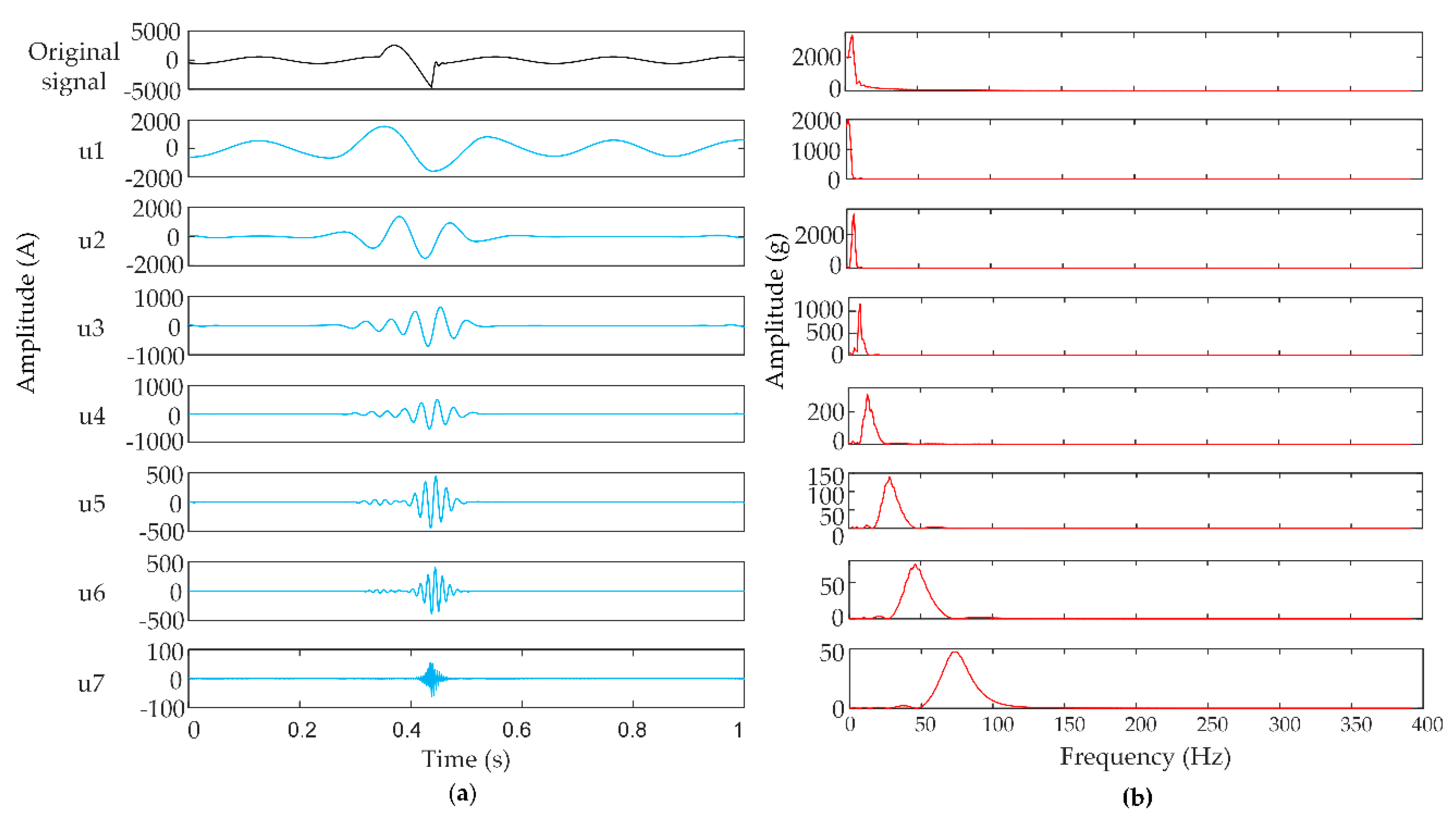
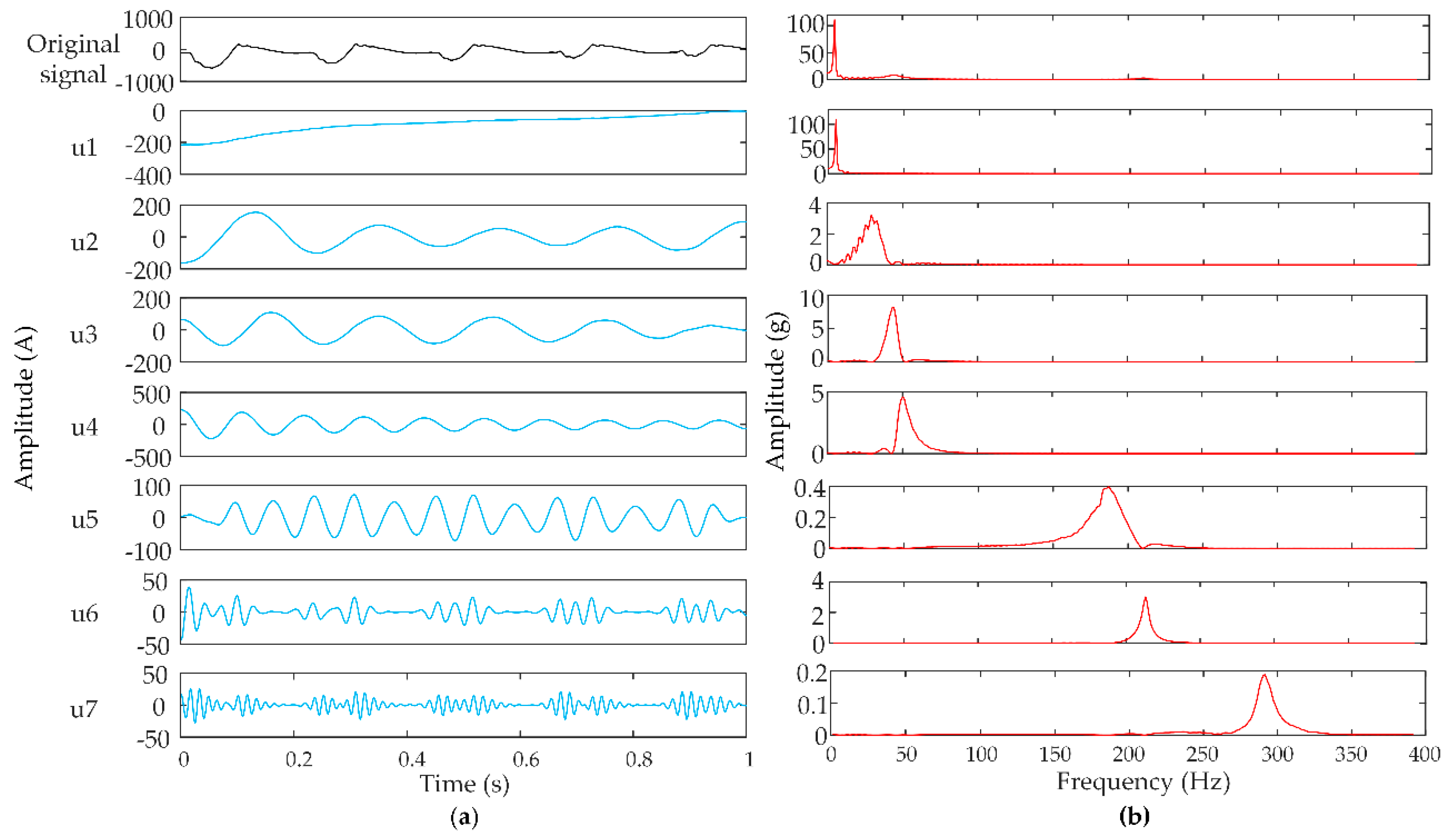
The number of decomposed modes K: VMD needs to preset the number of decompose modes K. If K is too small, the decomposed modes are too few, and all the decomposition modes cannot be captured; while if the value of K is too large, the interfering signal will be overdecomposed such that the center frequencies of modes will be mixed. By repeated observation in the experiment, the maximum center frequency and the minimum center frequency of the six types of signals are nearly constant when K = 7, and there is no large fluctuation with increasing decomposition mode, so K = 7 is used.

Due to space limitations, only Figure 6 and Figure 7 show the results and spectra of VMD for multicycle incipient cable failure and transformer inrush disturbance; the analysis process of other signals is similar. It is obvious that the waveforms of each mode corresponding to different signals differ greatly. Regarding spectra, two types of signals composed of low-frequency and intermediate-frequency content are better decomposed by VMD, so that it is fully prepared for subsequent feature extraction.

Figure 8 displays feature vectors FV_k obtained via VMD-based stratification extraction method for a total of 42 features. As the figure shows, in each mode, the same features of different signals are mostly distinct. For example, the first feature of each vector represents F1, and there are significant differences in the u1–u7 modes of different signals. F6 is the last term of each feature vector; although it is not changed in the u1–u3 modes of different signals, there is a certain difference in u3–u7. Therefore, these feature vectors can be used as the basis for different signal diagnostics and thus input into the CNN for recognition and classification.

The structure of the CNN has an important impact on the network performance and output accuracy. Considering the computational complexity and accuracy, the parameters that are more effective for simulation data are finally selected in this paper, as indicated in

Table 1. The parameters of the CNN model.

Layer Name	Kernel Size	Output Size
Input layer		1 × 42 × 1
Convolutional layer 1	1 × 3	1 × 40 × 18
Downsampling layer 1	1 × 2	1 × 20 × 18
Convolutional layer 2	1 × 6	1 × 15 × 14
Downsampling layer 2	1 × 5	1 × 3 × 14
Fully connected layer		1 × 42 × 1
Output layer		6 classes

. At the same time, the learning rate is set to 1, with 60 samples for each training and more than 30,000 iterations. In theory, the more iterations of the deep learning network, the higher the accuracy. In Figure 9, the impact of iteration number on classification results is shown.

The distribution of training samples for the entire experiment is reported in

Table 2. The number of samples.

Type	The Number of Samples	Training Samples	Test Samples
Subcycle incipient failure	2800	2100	700
Multicycle incipient failure	2800	2100	700
Normal signal	2800	2100	700
Transformer inrush	2800	2100	700
Constant impedance	2800	2100	700
Capacitor switching	2800	2100	700

.

For the final classification results of the subcycle incipient cable failure, multicycle incipient cable failure, normal signal, transformer inrush disturbance, constant impedance failure and capacitor switching disturbance, the performance of the model is presented in the form of a confusion matrix. As shown in Figure 10, the overall prediction accuracy is 96.1%. The rows represent the output labels, the columns represent the target labels, and the diagonal represents the number of samples correctly classified for each class. The results show that the most common mistake is to classify multicycle incipient failure as constant impedance failure; the recognition rate of multicycle incipient failure is 91.4%. The recognition rate of the normal signals is all correct, achieving 100%.

As reported in

Table 3. Comparison between VMD feature extraction and the original signals.

Preprocessing	CNN Training Time (s)	Classification Accuracy (%)
Feature extraction based on VMD	902.50	96.1
The original signals	8873.96	98.6

, in order to verify the validity of the proposed approach, the original signals are used directly as the CNN input to compare with feature extraction based on VMD.

Although the classification accuracy based on VMD feature extraction is 2.5% less than the direct classification, the training time is substantially shortened by 2.2 h. The reason for this result is that the proposed approach reduces the dimensionality of the data and the complexity of network calculation by VMD feature extraction, which shortens the classification time, but it is inevitable that some feature information is lost. In addition, Gaussian white noise is added to the original signals and show the classification results at a 15 dB, 20 dB and 25 dB signal-to-noise ratio (SNR) in

Table 4. Classification accuracy under Gaussian white noise.

Methods	Classification Accuracy (%)
	15 dB	20 dB	25 dB
Feature extraction based on VMD + CNN	83.52	89.33	93.21
The original signals + CNN	16.88	65.90	82.76

.

As reported in Table 4, the lower the SNR is, the better the robustness of the proposed approach. In particular, when the SNR is 15 dB, the original signals directly input into the CNN cannot be distinguished. However, the accuracy of the proposed approach is still as high as 83.52%. Thus, the results show that the VMD algorithm can accurately recognize failure under high-noise conditions.

To verify the effectiveness of the CNN model as a classifier, the classification results of four traditional classifiers (DT, KNN, BP and SVM) and the CNN are evaluated using the same training samples and test samples (as reported in

Table 5. Comparison of different classifiers.

Classifiers	Accuracy (%)
Feature extraction based on VMD + DT	85.31
Feature extraction based on VMD + KNN	93.45
Feature extraction based on VMD + BP	79.10
Feature extraction based on VMD + SVM	80.74
Feature extraction based on VMD + CNN (ours)	96.10

).

In Table 5, the classification accuracy of DT is 85.31%, that of KNN is 93.45%, that of BP is 79.1%, and that of SVM is 80.74%. Compared with the other three traditional algorithms, KNN has better classification results, but its accuracy is still less than that of the proposed approach. This result occurs because in the proposed approach, the CNN performs quadratic feature extraction by convolution before providing output as a classifier; by obtaining additional depth information, it can accurately realize recognition and classification. On the other hand, the advantage of the CNN is that although it takes considerable time in data training, once the training model is completed, it maintains good predictability and adaptability to analyze the same type of data.

4. Discussion

The results reported in Section 3 show that the spectra of incipient cable failures and overcurrent disturbance signals consist of different frequency components. Therefore, the method of extracting fine time-frequency information by VMD separating different frequency components is reliable. Second, the classification results show that the feature extraction method based on mathematical statistics after VMD can effectively shorten the training time of the CNN.

The comparison results under noise conditions also show that the original signal is difficult to distinguish under the influence of high noise. Therefore, VMD improves the robustness of failure recognition by filtering high-frequency noise, resulting in more accurate classification results.

On the other hand, the comparison results of different classifiers show that the CNN, as a classifier with feature processing ability, can provide higher possibility of accurate classification.

Finally, it is worth noting here that the proposed approach is based only on simulated signals. Although all simulation samples were generated based on the actual interference waveform, more validation is needed if the approach is to be successfully applied to actual measurements.

5. Conclusions

To solve the problem that incipient cable failures are difficult to distinguish from overcurrent disturbances, an approach for the recognition and classification of incipient cable failures based on VMD and a CNN is proposed. First, the original signal is decomposed to obtain component signals containing more waveform features, and then the eigenvalues are calculated by analyzing the characteristics of the different signals; the results are used to construct an the input vector of the CNN. Finally, by training the CNN, recognition and classification of initial cable failure is achieved.

The approach makes full use of the noise immunity of VMD and the self-learning of the CNN, so achieves reliable and accurate classification. The effectiveness of the proposed approach is verified using different classifiers and high noise. The experimental results show that the approach has high precision and robustness.

References

1. Tang, Z.; Zhou, C.; Jiang, W. Analysis of Significant Factors on Cable Failure Using the Cox Proportional Hazard Model. IEEE Trans. Power Deliv. 2014, 29, 951–957. [Google Scholar] [CrossRef]
2. Bretas, A.S.; Herrera-Orozco, A.R.; Herrera-Orozco, C.A. Incipient fault location method for distribution networks with underground shielded cables: A system identification approach. Int. Trans. Electr. Energy Syst. 2017, 27, e2465. [Google Scholar] [CrossRef]
3. Zhang, W.; Xiao, X.; Zhou, K. Multi-Cycle Incipient Fault Detection and Location for Medium Voltage Underground Cable. IEEE Trans. Power Deliv. 2016, 32, 1450–1459. [Google Scholar] [CrossRef]
4. Charytoniuk, W.; Lee, W.J.; Chen, M.S. Arcing fault detection in underground distribution networks-feasibility study. IEEE Trans. Ind. Appl. 2000, 36, 1756–1761. [Google Scholar]
5. Pavlatos, C.; Vita, V.; Dimopoulos, A.C.; Ekonomou, L. Transmission lines’ fault detection using syntactic pattern recognition. Energy Syst. 2018, 10, 299–320. [Google Scholar] [CrossRef]
6. Pavlatos, C.; Vita, V. Linguistic representation of power system signals. In Electricity Distribution; Energy Systems Series; Springer: Berlin/Heidelberg, Germany, 2016; pp. 285–295. [Google Scholar]
7. Xu, J.; Baese, U.M.; Huang, K. FPGA-based solution for real-time tracking of time-varying harmonics and power disturbances. Int. J. Power Electron. 2012, 4, 134. [Google Scholar] [CrossRef]
8. Romano, P.; Imburgia, A.; Ala, G. Partial Discharge Detection Using a Spherical Electromagnetic Sensor. Sensors 2019, 19, 1014. [Google Scholar] [CrossRef]
9. Nuruzzaman, A.; Boyraz, O.; Jalali, B. Time-stretched short-time Fourier transform. IEEE Trans. Instrum. Meas. 2006, 55, 598–602. [Google Scholar] [CrossRef]
10. Debnath, L. Wavelet Transforms and Time-Frequency Signal Analysis. Wavelet Transforms and Time-Frequency Signal Analysis; Birkhäuser: Boston, MA, USA, 2001. [Google Scholar]
11. Huang, N.E.; Shen, Z.; Long, S.R.; Wu, M.C.; Shih, H.H.; Zheng, Q.; Yen, N.-C.; Tung, C.C.; Liu, H.H. The Empirical Mode Decomposition and the Hilbert Spectrum for Nonlinear and Non-Stationary Time Series Analysis. Proc. Math. Phys. Eng. Sci. 1998, 454, 903–995. [Google Scholar] [CrossRef]
12. Cheng, H.; Chen, X.; Liu, F.; Wang, C. Series Arc Fault Detection and Implementation Based on the Short-time Fourier Transform. In Proceedings of the Asia-Pacific Power and Energy Engineering Conference, Chengdu, China, 28–31 March 2010. [Google Scholar]
13. Sidhu, T.S.; Xu, Z. Detection of Incipient Faults in Distribution Underground Cables. IEEE Trans. Power Deliv. 2010, 25, 1363–1371. [Google Scholar] [CrossRef]
14. Zhang, C.; Kang, X.N.; Ma, X.D. On-line Incipient Faults Detection in Underground Cables Based on Single-end Sheath Currents. In Proceedings of the Power & Energy Engineering Conference, Suzhou, China, 15–17 April 2016. [Google Scholar]
15. Gu, F.C.; Chang, H.C.; Chen, F.H. Application of the Hilbert-Huang transform with fractal feature enhancement on partial discharge recognition of power cable joints. IET Sci. Meas. Technol. 2012, 6, 440–448. [Google Scholar] [CrossRef]
16. Dragomiretskiy, K.; Zosso, D. Variational Mode Decomposition. IEEE Trans. Signal Process. 2014, 62, 531–544. [Google Scholar] [CrossRef]
17. Zhang, J.; He, J.; Long, J.; Yao, M.; Zhou, W. A New Denoising Method for UHF PD Signals Using Adaptive VMD and SSA-Based Shrinkage Method. Sensors 2019, 19, 1594. [Google Scholar] [CrossRef] [PubMed]
18. Achlerkar, P.D.; Samantaray, S.R.; Manikandan, M.S. Variational Mode Decomposition and Decision Tree Based Detection and Classification of Power Quality Disturbances in Grid-Connected Distributed Generation System. IEEE Trans. Smart Grid 2018, 9, 3122–3132. [Google Scholar] [CrossRef]
19. Voumvoulakis, E.M.; Gavoyiannis, A.E.; Hatziargyriou, N.D. Application of Machine Learning on Power System Dynamic Security Assessment. In Proceedings of the International Conference on Intelligent Systems Applications to Power Systems, Taiwan, China, 5–8 November 2007. [Google Scholar]
20. Tang, J.; Jin, M.; Zeng, F.; Zhou, S.; Zhang, X.; Yang, Y.; Ma, Y. Feature Selection for Partial Discharge Severity Assessment in Gas-Insulated Switchgear Based on Minimum Redundancy and Maximum Relevance. Energies 2017, 10, 1516. [Google Scholar] [CrossRef]
21. Mas’ud, A.; Albarracín, R.; Ardila-Rey, J.; Muhammad-Sukki, F.; Illias, H.; Bani, N.; Munir, A. Artificial Neural Network Application for Partial Discharge Recognition: Survey and Future Directions. Energies 2016, 9, 574. [Google Scholar] [CrossRef]
22. Mas’ud, A.; Ardila-Rey, J.; Albarracín, R.; Muhammad-Sukki, F.; Bani, N. Comparison of the Performance of Artificial Neural Networks and Fuzzy Logic for Recognizing Different Partial Discharge Sources. Energies 2017, 10, 1060. [Google Scholar] [CrossRef]
23. Parrado-Hernández, E.; Robles, G.; Ardila-Rey, J.; Martínez-Tarifa, J. Robust Condition Assessment of Electrical Equipment with One Class Support Vector Machines Based on the Measurement of Partial Discharges. Energies 2018, 11, 486. [Google Scholar] [CrossRef]
24. Shan, S. Decision Tree Learning. In Machine Learning Models and Algorithms for Big Data Classification; Springer: New York, NY, USA, 2016; pp. 237–269. [Google Scholar]
25. Zhang, S.; Wang, Y.; Liu, M. Data-based Line Trip Fault Prediction in Power Systems Using LSTM Networks and SVM. IEEE Access 2017, 6, 7675–7686. [Google Scholar] [CrossRef]
26. Cai, L.; Thornhill, N.; Kuenzel, S. Real-time Detection of Power System Disturbances Based on k-Nearest Neighbor Analysis. IEEE Access 2017, 5, 5631–5639. [Google Scholar] [CrossRef]
27. Maryam, M.N.; Flavio, V.; Taghi, M.K. Deep learning applications and challenges in big data analytics. J. Big Data 2015, 2, 1. [Google Scholar] [Green Version]
28. Wang, Y.; Liu, M.; Bao, Z. Deep learning neural network for power system fault diagnosis. In Proceedings of the 2016 35th Chinese Control Conference (CCC), Chengdu, China, 27–29 July 2016. [Google Scholar]
29. Hinton, G.E.; Osindero, S.; Teh, Y.W. A Fast Learning Algorithm for Deep Belief Nets. Neural Comput. 2014, 18, 1527–1554. [Google Scholar] [CrossRef]
30. Zhou, G.B.; Wu, J.; Zhang, C.L.; Zhou, Z.H. Minimal gated unit for recurrent neural networks. Int. J. Autom. Comput. 2016, 13, 226–234. [Google Scholar] [CrossRef] [Green Version]
31. Nguyen, M.; Nguyen, V.; Yun, S.; Kim, Y. Recurrent Neural Network for Partial Discharge Diagnosis in Gas-Insulated Switchgear. Energies 2018, 11, 1202. [Google Scholar] [CrossRef]
32. LeCun, Y.; Bottou, L.; Bengio, Y.; Haffner, P. Gradient-based learning applied to document recognition. Proc. IEEE 1998, 6, 2278–2324. [Google Scholar] [CrossRef]
33. Cheng, J.; Wang, P.S.; Gang, L.I. Recent advances in efficient computation of deep convolutional neural networks. Front. Inf. Technol. Electron. Eng. 2018, 19, 64–77. [Google Scholar] [CrossRef] [Green Version]
34. Bertsekas, D.P. Constrained Optimization and Lagrange Multiplier Methods; Academic Press: Cambridge, MA, USA, 1982; p. 104. [Google Scholar]
Figure 1. Main structure of the proposed incipient cable failure recognition and classification process.
Energies 12 02005 g001
Figure 2. Structure of the CNN with two convolutional layers.
Energies 12 02005 g002
Figure 3. The flowchart based on VMD and CNN.
Energies 12 02005 g003
Figure 4. Simulation model of incipient cable failure and the overcurrent interference signals.
Energies 12 02005 g004
Figure 5. Current waveforms of incipient cable failure, normal signal and overcurrent interference: (a) Subcycle incipient cable failure (b) Multicycle incipient cable failure (c) Normal signal (d) Transformer inrush disturbance (e) Constant impedance failure (f) Capacitor switching disturbance.
Energies 12 02005 g005
Figure 6. Results and spectra of VMD for multicycle incipient cable failure: (a) Modes; (b) Frequency spectra.
Energies 12 02005 g006
Figure 7. Results and spectra of VMD for transformer inrush disturbance: (a) Modes; (b) Frequency spectra.
Energies 12 02005 g007
Figure 8. Feature extraction based on VMD: (a)–(g) denotes the respective feature vector FVk of the u1–u7 decomposed modes. (h) denotes the representation of different signal types.
Energies 12 02005 g008aEnergies 12 02005 g008b
Figure 9. Impact of the iteration number on the results.
Energies 12 02005 g009
Figure 10. The results of the classification confusion matrix based on VMD and CNN.
Energies 12 02005 g010