A Study on the Effect of Closed-Loop Wind Farm Control on Power and Tower Load in Derating the TSO Command Condition

Abstract

This study was conducted to analyze the impact of surrounding environmental changes on the feedback gain and performance of a closed-loop wind farm controller that reduces the error between total power output of wind farm and power command of transmission system operator. To analyze the impact of environment changes on wind farm controller feedback gain, the feedback gain was manually changed from 0 to 0.9 with a 0.1 interval. In this study, wind speed and wind direction changes were considered as environment changes; it was found by simulation code that the wind farm controller gain is in inverse proportion to wake recovery rate. In other words, the feedback gain should be higher if the distance between upstream and downstream wind turbine is not sufficient to wake recovery. Furthermore, the feedback gain should be lower when the upstream wind turbine generates a relatively weak wake by operating above the rated wind speed. The wind farm simulation was performed using reference 5 MW wind turbines from the National Renewable Energy Laboratory (NREL), which are numerically modeled for each element so that wind farm power output and tower load can be calculated according to the variation of the power command by using a modified wake model with improved accuracy. All the simulations performed in this study were carried out to review the power output accuracy of wind farms, but only if the transmission system operator’s power command was lower than the available power of wind farm. In this study, the gain of the wind farm controller was applied differently depending on the wind speed and direction to consider benefits in terms of power and tower load, especially if the wake effect of the upstream wind turbine was rapidly transferred to the downstream wind turbine. Ultimately, a simple, but more effective, power distribution method was proposed for distributing power commands to wind turbines that constitute wind farms and the study indicated the need for controller gain adjustment based on surrounding environmental changes.

1. Introduction

Among power generation technologies that utilize renewable energy sources wind power generation is known to have relatively mature technology and high efficiency. As a result, more than 50 GW of wind turbines have been installed over the world annually since 2015 and the cumulative installed capacity of wind power exceeded 539 GW in 2017 [1].

The cost of energy generated by wind power, which can be calculated by dividing the sum of the capital expenditure (CAPEX) and operating expenses (OPEX) for twenty years by the total power production, has been continuously reduced as the technology evolves further and further. Based on a recent report, wind farms larger than 300 MW have been found to be comparable, or even superior, to fossil fuel-based power generation in terms of cost of energy (COE) [2].

Although the COE of wind power generation has been substantially reduced, offshore wind power is much more expensive than its onshore counterpart. For this reason, many researchers have been working to lower the COE of wind power [3,4,5,6,7,8,9,10,11,12,13,14,15].

Wind turbine clustering, or installing a wind farm rather than a single turbine installation, is a basic method for reducing COE by increasing the cost efficiency of power generation. Additionally, the layout optimization of a wind farm is a well-known way of reducing COE by improving its annual power output. As wind passes through a turbine, its speed is reduced and its turbulence is increased due to the interaction with the rotating rotor. This phenomenon, known as wake, reduces the power output of wind turbines installed downstream. Thus, wind turbines are installed in a way that minimizes the wake effect between wind turbines, taking into account the prevailing wind direction at the site [3,4,5].

Wind turbine clustering and layout optimization are both simple and effective methods for reducing the COE of wind energy. However, since these methods are only applicable at the beginning stage of wind farm development, the reduction of COE through these two methods is limited. For this reason, wind farm control studies have been actively conducted to improve the power output of wind farms that have already been installed and are in operation [6,7,8,9,10,11,12,13,14,15].

Wind farm control can be divided into two types based on function: active power control and reactive power control [16].

With regard to active wind farm control, it has been used to match the total power output from a wind farm to the power demand from the transmission system operator (TSO) when power derating is needed [17]. It can be done with a proportional control strategy either through open-loop control or proportional-integral (PI) feedback closed-loop control [18]. More recently, new algorithms for active power control have been proposed to increase the total power output of wind farms by adjusting the wake from upstream wind turbines when power derating is not needed. However, the effectiveness of gaining total power increase through active wind farm control has been debated [6,7,8,9,10,11,12,13,14,15].

The conventional power command distribution model has focused mostly on reducing the error between the power output of a wind farm and the power command from the TSO without considering the fatigue load. Recently, different methods have been proposed for power command distribution to yield a reduction in COE [19,20,21,22,23].

Zhao et al. applied the model predictive control (MPC) method to control active power and verified its performance with a wind farm simulation tool. The authors proposed not only a method of power command distribution but also a wind farm controller [19,20]. The proposed wind farm controller consists of a high-level controller that operates at a relatively low frequency and a model predictive control (MPC)-based low-level wind farm controller that operates at a high frequency. To verify the performance of the proposed controller, the authors compared the proposed controller with the traditional proportional distribution model based wind farm controller. As a result, the fluctuation in the power output and structural load was reduced through the use of the proposed controller. However, it was not a feedback controller, and therefore it has limitations due to its open-loop characteristics.

Zhang et al. applied optimization algorithms, including the genetic algorithm and improved binary particle swarm algorithm, to their wind farm controller and verified the power output and mechanical load variation through simulation [21]. In their study, the power output of the wind farm was controlled by the shutdown and power derating of the turbines. The authors verified that the overall lifetime of the wind farm was increased by forcibly stopping unnecessary wind turbines when two optimization algorithms were used in combination. However, even if a high-level optimization algorithm is applied, the error between the power output and power command by the TSO was relatively large.

Although previous wind farm controller studies have proposed various methods for active power control and verified the performance through simulation, they are limited in that they are using simple wind turbine models in their simulations. Guo et al. improved the accuracy of the wind turbine model of the previous studies and reinvestigated the MPC technique-based wind farm controller [22]. The authors simulated the wind farm using a wind turbine numerical model that controls the blade pitch angle and generator torque according to changes in the external power command. The authors also proposed a method of applying a communication-based MPC to the wind farm controller. In the study, the power output and structural load fluctuations were reduced through the proposed controller. However, since the proposed wind farm controller was not a closed-loop, and therefore, has limitations due to its open-loop characteristics.

The recent study by Boersma et al. proposed a wind farm controller that combines wake steering control algorithm and active power control techniques based on the MPC technique to improve the output of wind farms [23]. The proposed wind farm controller was designed to control the power output of the wind farm through active power control when the power command of the TSO is less than the available power and activate the wake steering control algorithm in the opposite scenario to improve the overall power output. The proposed wind farm controller was verified by using large eddy simulation (LES) technique-based wind farm simulation code. However, although wind farm simulations have been carried out through LES, they did not take into account different scenarios with variations in wind speed and direction due to the computational time that would be required. As a result, the performance change of the wind farm controller according to the environmental changes was not considered.

This study was carried out considering the limitations of the previous studies mentioned above.

First, this study proposes a simple but effective method of wind farm control that is as simple as the well-known and already-applied method of proportional wind farm control and is as effective as closed-loop control in matching the power command by the TSO and reducing the tower loads.

Second, to verify the performance of the proposed wind farm controller, this study constructed a wind farm in-house simulation code based on a MATLAB/Simulink-based wind turbine model and a wake model with improved wake prediction accuracy through a wind tunnel test. The wind turbine model applied to the simulation code was designed to simulate the operational state change of the wind turbine according to the wind speed and change in the external power command with the demanded power point tracking algorithm. In addition, the empirical model, which simulates the influence of the momentum of turbulence change on the wake region, was modified through the wind tunnel test and applied to the simulation code to obtain highly reliable simulation results.

Third, in this study, the authors confirmed the performance change of the proposed wind farm controller through simulation scenarios designed to consider various environmental changes. In particular, this study clarifies the performance and limitations of the proposed wind farm controller by simulating the power output performance and the tower load variation of the wind farm according to the change in wind speed, direction, and wind farm controller gain. In this study, the simulation scenarios were planned by combining four different wind directions and two wind speeds, and simulations were performed by applying ten different wind farm controller gains.

Although this study simulates various conditions considering different wind speeds, directions, and wind farm controller gains, it was still limited because it did not consider the continuous change of wind direction in the time domain. Additionally, the wake model applied to the wake simulation code could be different from the wake generated in the actual environment because the model was developed assuming axial symmetry, etc.

2. Wind Farm Modeling and Simulation

2.1. Wind Farm Simulation Code

Wind farm simulations were performed using an in-house simulation code that has a similar structure to SimWindFarm [24,25]. Despite this similar structure, it was designed to have a higher accuracy by applying the modified wake model, wake deflection model, wake propagation delay due to environmental changes, etc. The simulation code was constructed in C language and can be simulated relatively quickly [25].

As shown in Figure 1, the wind farm in-house simulation code simulates a wind farm by inputting some of the wind farm information such as the coordinates of the turbines, turbulence wind data, wind direction data, and TSO commands. The simulation code calculates changes in the dynamic behavior of the wind turbines, such the power output, blade pitch angle, rotor speed, etc., at 0.1 s intervals.

Wind turbine models in simulation tools are inputted with reduced wind due to wake effect as well as terrain effect. The terrain effect used in this study was constructed by using CFD simulation result of WindSim, which is a commercial wind farm simulation tool to predict annual power production. The CFD simulation result includes wind speed variation data at each point according to ground height increase. Also, the interaction between wind turbines was implemented based on the modified Ainslie Eddy Viscosity Wake model [26]. Where, the wake calculation is performed regardless of the location of the installation of the wind turbine and only valid wake data to be delivered to the wind turbine located relatively downstream is stored separately.

Separately stored valid wake data is transmitted to downstream wind turbines by reflecting the wake propagation delay time calculated considering the distance between the wind turbines, the ambient wind speed, and the operation state of the wind turbine. The wind turbine simulation tool repeatedly performs this process and interprets the change in behavior of each wind turbine in the time domain. A description of the wake model, wake deflection model, time delay model, and terrain model applied to the simulation tool, including the wind turbine model, has been reviewed in the following chapters.

One of the features of the in-house wind farm simulation code is that it works with a wind farm controller with various algorithms. The wind farm modeled through the simulation code is configured to not only transmit the states of each turbine to the controller but also to receive the output command per turbine from the linked controller. With this configuration, the simulation code can simulate the power output and tower load change of the wind farm according to the control algorithm and control gain installed in the controller.

2.1.1. Wind Turbine Model

All wind turbines operate on the basis of the aerodynamic torque coefficient, thrust coefficient, and controller installed on each turbine based on the blade element momentum (BEM) theory. The wind turbine model was designed to control the blade pitch angle and generator torque to reduce the error between the inputted power command and actual power output when the output power requirement is lower than the available power. The wind turbine model was modeled using MATLAB/Simulink, and the generator, the drive train, pitch actuator, and tower were composed of a primary or secondary dynamic submodel.

The accuracy of the used wind turbine model was verified by previous studies [25]. As Figure 2 shows, the wind turbine model is designed to operate in accordance with the wind speed and power command. Wind turbine models, especially those applied to simulation tools, undergo turbulent winds with both terrain and wake effects, depending on the location of the wind turbine installation. The wind turbine simulation uses this type of wind turbine model to simulate changes in wind turbine behavior in time domain. Also, as shown in Figure 2, the controller installed in the wind turbine numerical model calculates the generator torque and blade pitch angle needed to reach the power command by receiving the generator speed, blade pitch angle, and power output amount according to the inputted wind speed.

The controller in the wind turbine model can implement advanced mechanical load control algorithms such as peak shaving or tower damper. However, in this study, the influence of wind farm control gain on the power output and tower load was investigated using only the basic demanded power point tracking (DPPT) algorithm. A detailed description of the DPPT control algorithm applied to the wind turbine model can be found in Ref. [27].

2.1.2. Wake Model

The simulation code calculates the wake using the modified Ainslie eddy viscosity wake model with improved wake prediction accuracy through a wind tunnel test based on a scaled turbine model with similar operating characteristics to an MW-class turbine. The wake model was modified using the filter function to account for the initial wind profile and momentum of turbulence change in the wake region [26].

The modified wake model has the same limitations as the original wake model with regard to wake calculation because it computes uses the same governing equations as the original Ainslie eddy viscosity wake model shown in Equation (1) [28].

$$U\frac{\partial U}{\partial x}+V\frac{\partial U}{\partial r}=-\frac{1}{r}\left(\frac{\partial \left(r\overline{u{}^{\prime }v{}^{\prime }}\right)}{\partial r}\right)$$

(1)

where r is the distance from the center of the rotor, x is the downstream distance, $U$ is the longitudinal direction wind speed, $V$ is the lateral direction wind speed, and $\overline{u{}^{\prime }v{}^{\prime }}$ is the Reynolds stress. The initial wind profile, U_INP, required for wake calculation, was calculated by the following Equations (2)–(4) [26].

$$U_{INP}=\{\begin{array}{cc}{P}_1{D}_M\cos (r)\exp (-P_{2}r)+1& ,r<0.7\\ 1& ,r\ge 0.7\end{array}$$

(2)

$$k=\frac{r}{P_2}+\left(D_M-0.746\right)+P_4\sin (\frac{r}{P_5}-P_6)$$

(3)

$$D_M=C_T-0.05-\frac{\left(16C_T-0.5\right)TI}{10}$$

(4)

where $P_{1-6}$ are the parameters derived from the wind tunnel test, $C_T$ is the thrust coefficient, and TI is the atmospheric turbulence intensity. All of the parameters used in the model are presented in Ref. [26]. The thrust coefficient and turbulence intensity are defined by Equations (5) and (6), respectively.

$$C_T=\frac{\begin{array}{cc}Thrust& Force\end{array}}{\begin{array}{cc}Aerodynamic& Force\end{array}}=\frac{F}{\frac{1}{2}\rho A{U}^2}$$

(5)

$$TI=\frac{\partial U}{\overline{U}}$$

(6)

where ${\sigma }_U$ and $\overline{U}$ denote the standard deviation of wind speed and mean wind speed, respectively.

2.1.3. Wake Deflection Model

On the wind farm, changes in wind direction instantaneously cause yaw errors. This error not only reduces the output of individual wind turbines but also changes the direction of wake propagation. Therefore, the wake deflection phenomenon needs to be considered to simulate the change in wind direction occurring in the time domain. The applied wake deflection model was proposed by Jiménez et al. and calculates the wake deflection phenomenon caused by the yaw. The wake deflection model is given by Equation (7) [29].

$$\alpha =\frac{{\cos }^2\psi \sin \psi \frac{C_T}{2}}{1+\gamma \frac{x}{D}}$$

(7)

where $\alpha$ is the angle of wake deflection along the distance, $\psi$ is the yaw error, $\gamma$ is a constant for calculation, and D is the wind turbine diameter. In this study, 0.125 was applied to $\gamma$.

2.1.4. Wind Propagation with Time Delay

In this study, the time delay model used in Gebraad et al. was applied to the wind farm in-house simulation code to implement the wake propagation time delay between wind turbines. The time delay model was designed by the actuator disk theory and used to calculate the delay time of wake propagation. The delay time was calculated by Equation (8) [30].

$$t_{delay}=-\frac{\Delta x}{\frac{1}{2}\left(U_i\left(1-2a_i\right)+U_{i+1}\right)}$$

(8)

where $∆x$ is the distance between the ith and i + 1th wind turbine and a is the induction factor. The relationship between the induction factor and thrust coefficient is given by Equation (9).

$$C_T=4a\left(1-a\right)$$

(9)

The wake superposition phenomena were realized by the sum of squares of the velocity deficit model. This model is also used in commercial wind farm simulation tools such as WindPRO; the governing equation is given in Equation (10) [31].

$$Defici{t}_n=\sqrt{{\displaystyle \sum _{i=1}^{n-1}{\left(Defici{t}_{i,n}\right)}^2}}$$

(10)

where $Defici{t}_{in}$ indicates the wake strength of the ith wind turbine on the nth wind turbine. Deficit is defined by Equation (11).

$$Deficit=\frac{\Delta U}{U_{\infty }}$$

(11)

2.1.5. Terrain Modeling

In this study, the terrain model, computed by a commercial CFD analysis program, was applied to the simulation code to improve the accuracy of wind field prediction. The applied terrain model was constructed by using commercial software WindSim, which simulates annual energy production of wind farm based on CFD analysis. WindSim uses universal CFD code Phoenics and needs the terrain geometric information for calculating the variation of wind field on the surface of terrain with different azimuth angle.

The calculated CFD result were postprocessed and used to construct four dimensional look-up table and applied to the code.

2.1.6. Wind Farm Modeling

In this study, a 5 MW reference wind turbine model from the National Renewable Energy Laboratory (NREL) was used to provide detailed information on wind turbine modeling to consider the wind farm’s overall response and load variation according to the control setting change of the wind turbine controller.

Table 1. Specifications of the National Renewable Energy Laboratory (NREL) 5 MW wind turbine model [32].

Rotor diameter	126.0 m
Hub diameter	3.0 m
Hub height	90.0 m
Cut-in/rated/cut-out wind speed	3.0/11.4/25.0 m/s
Cut-in/rated rotor speed	6.9/12.1 rpm

shows the specification of NREL 5 MW reference wind turbine.

The wind farm was designed to accommodate twenty turbines. The spacing of the turbines was set to six times the rotor diameter in both lateral and longitudinal directions considering the typical distance of general offshore wind farms and the turbine coordinates were rotated to simulate changes in turbine spacing according to the different wind direction [33]. Figure 3 shows the wind farm layout according to the wind direction change applied to the simulation tool.

In this study, to verify wind field prediction accuracy of the in-house simulation code, a wind farm in is normal operation is modeled, and then the simulation result is compared with the actual measured data. The wind farm for verification is located flat terrain in the Republic of Korea and consists of 15 wind turbines with 2 MW capacity. Figure 4 shows the power curve and thrust coefficient of the wind turbine. Figure 4a shows the power curve of wind turbine and Figure 5b shows the thrust coefficient.

The wind speed and wind direction data measured from met-mast were used for wind farm simulation. Figure 5 below shows the layout of wind farm.

Table 2. Wind farm simulation code validation result.

ID	Error [%]	id	Error [%]
#1	2.57	#9	4.59
#2	8.95	#10	10.54
#3	15.88	#11	8.54
#4	16.75	#12	14.43
#5	8.52	#13	10.40
#6	2.44	#14	7.49
#7	7.96	#15	3.19
#8	10.53	AEP	7.97

shows the comparison result between actual measured data and simulation data. As shown from the result, the wind farm simulation code has relatively high accuracy to estimate wind turbine electrical power variation. The error in annual energy production (AEP) and electrical power of each wind turbines are presented in Table 2. As shown in Table 2, the accuracy of prediction of power generation through simulation code was higher in proximity to the met-mast tower. In addition, the farther the wind turbines were, the more accurate it was to predict power generation through simulation codes. The error in AEP estimation was 7.97%.

2.2. Wind Farm Controller

The wind farm controller was used to distribute the power command according to the TSO requirement. It was designed to operate based on a wind speed estimator, power command distribution algorithm, and simple wind farm model.

The wind speed estimator uses the measured wind turbine blade pitch angle, generator speed, and generator torque of each turbine and estimates the effective wind speed that affects each one.

The torque generated in the rotor is calculated by Equation (12) [34].

$$\left(J_r+N^2{J}_g\right)\frac{d{\dot{\theta }}_r}{dt}=T_a-N{T}_g-\left(B_r+N^2{B}_g\right){\dot{\theta }}_r$$

(12)

where $T_a$ is the aerodynamic torque generated in the rotor, J is the mass moment of inertia, N is the gearbox gear ratio, ${\dot{\theta }}_r$ is the rotational speed of the rotor, and B is the damping coefficient. The subscripts r, g, and a represent rotor, generator, and aerodynamic, respectively. The torque calculated through the Equation (12) can be substituted into Equation (13) to estimate the effective wind speed affecting the wind turbine [35].

$$T_a=\frac{1}{2}\rho \pi R^3\left(\frac{C_P\left(\lambda ,\beta \right)}{\lambda }\right)U_{eff}^2$$

(13)

where $\rho$ is the air density, R is the rotor radius, $C_P$ is the power coefficient derived from the BEM theory, $\lambda$ is the tip speed ratio, $\beta$ is the blade pitch angle, and $U_{eff}$ is the effective wind speed. The tip speed ratio is calculated by Equation (14).

$$\lambda =\frac{{\dot{\theta }}_{r}R}{U}$$

(14)

The wind speed estimated by the wind speed estimator was used to predict the available power ($P_{AV}$) of each wind turbine in the wind farm through Equation (15).

$$P_{AV}=T_a{\dot{\theta }}_r{\eta }_m{\eta }_g$$

(15)

where $\eta$ means efficiency. The subscripts AV and m represent available and mechanical, respectively.

In this study, two different power distribution models were used to investigate the variation of the power output and the load according to the different power command distribution model. The first of the models is the proportional distribution model, which divides the ratio of the available power of each wind turbine to the power command of the TSO by the power command for each turbine [36]. One of the characteristics of this model is that the power command is proportional to the available power of each wind turbine. However, this model is only useful if it is able to determine the available power of each wind turbine and it also has a high dependency on the accuracy of the estimated power output capacity.

Proportional distribution model was considered as the baseline distribution model because it distributes the output proportionally and considers only the reserve capacity of the individual turbines rather than the accuracy of the total power output or tower load efficiency of the wind farm. The power command for each wind turbine is distributed through Equation (16).

$$P_{CMD,i}^{Baseline}=\frac{P_{AV,i}}{{\displaystyle \sum P_{AV}}}TS{O}_{CMD}$$

(16)

The subscript CMD represents command.

The second power command distribution model is the equal distribution model. By using this model, all wind turbines have the same power command obtained by dividing the power command requested by the TSO into the number of turbines constituting the wind farm, as shown in Equation (17). This model is applicable to wind farms even if the available power of each wind turbine cannot be accurately estimated, unlike the proportional distribution model.

$$P_{CMD,i}^{ED}=\frac{TS{O}_{CMD}}{N}$$

(17)

where N is the number of turbines constituting the wind farm. The subscript ED represents equal distribution. Figure 6 shows the schematic of the wind farm controller.

The wind farm controller should be operated with enough time until the upstream wake moves to the downstream wind turbine [37]. Therefore, the operating interval time of the wind farm controller was set to 100 s in this study.

2.3. Wind Farm Simulation

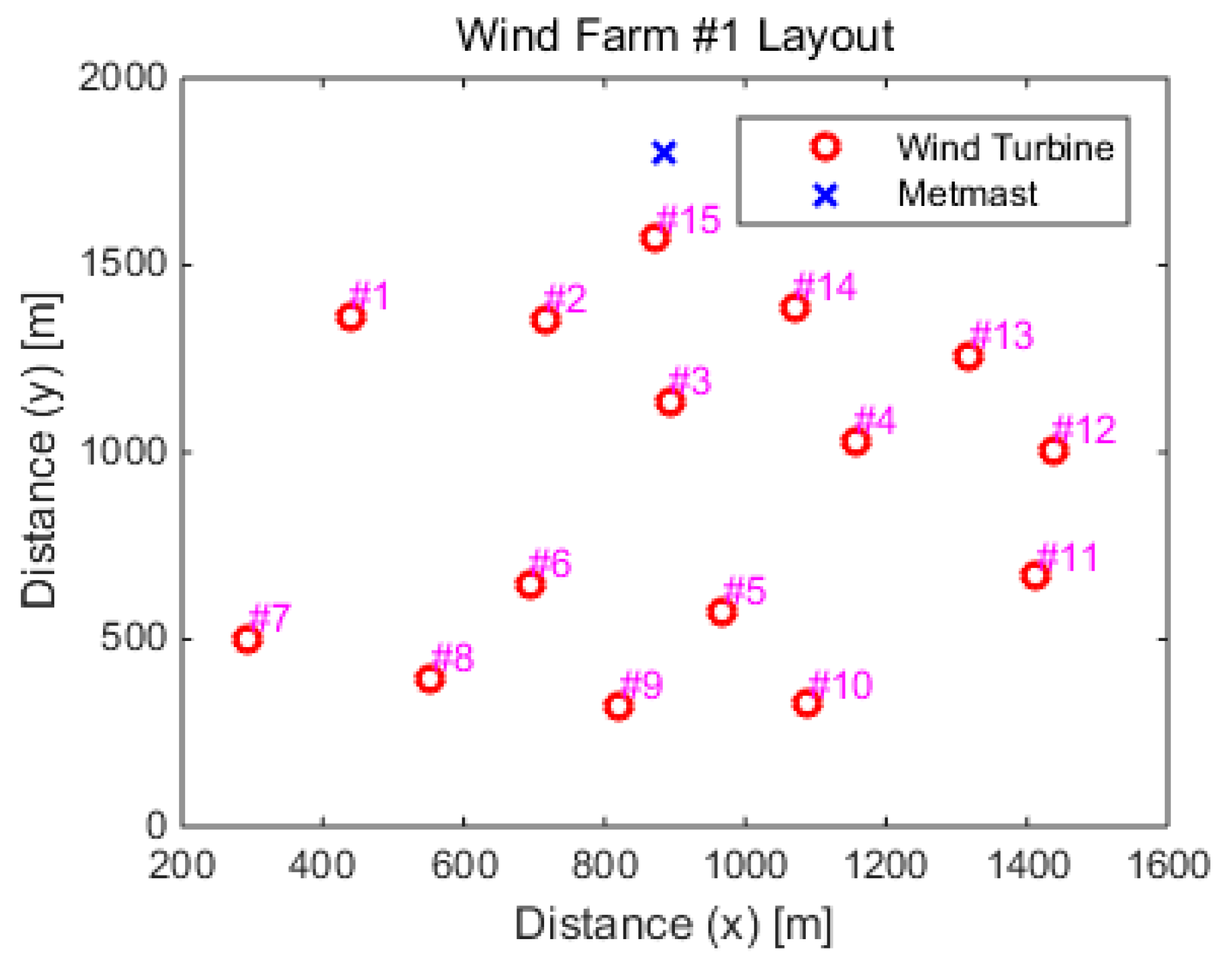
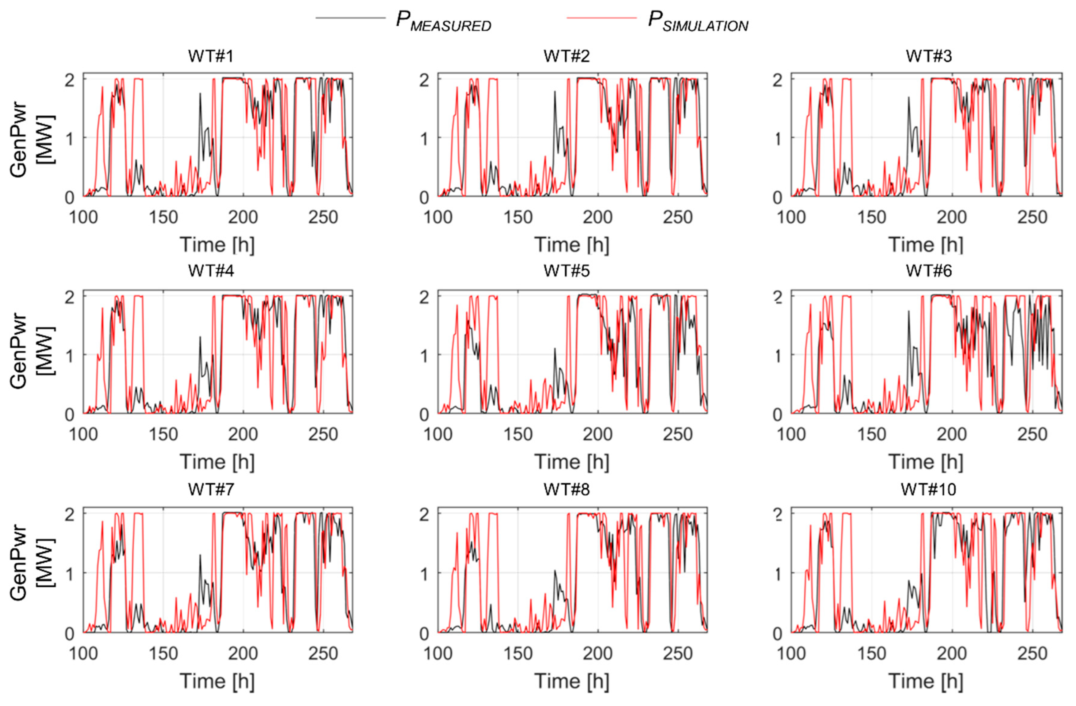
2.3.1. Wind Farm Simulation In-House Code Validation

Simulation accuracy of the wind farm in-house simulation code validation was performed by comparing the measured electrical power for one year and simulation results. Figure 7 shows the results of the comparison of measured electrical power with simulation result. As shown in the figure, the accuracy of the wind farm in-house simulation code has high fidelity. As a result of comparison with the measured data, the error of total electrical power production was 6.7%.

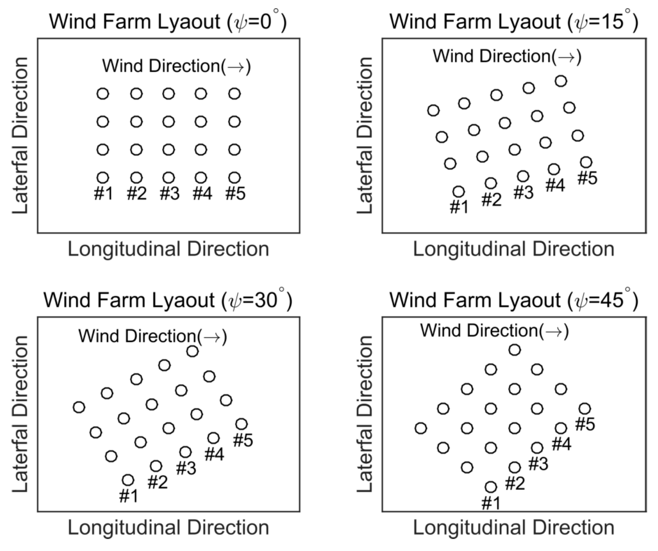
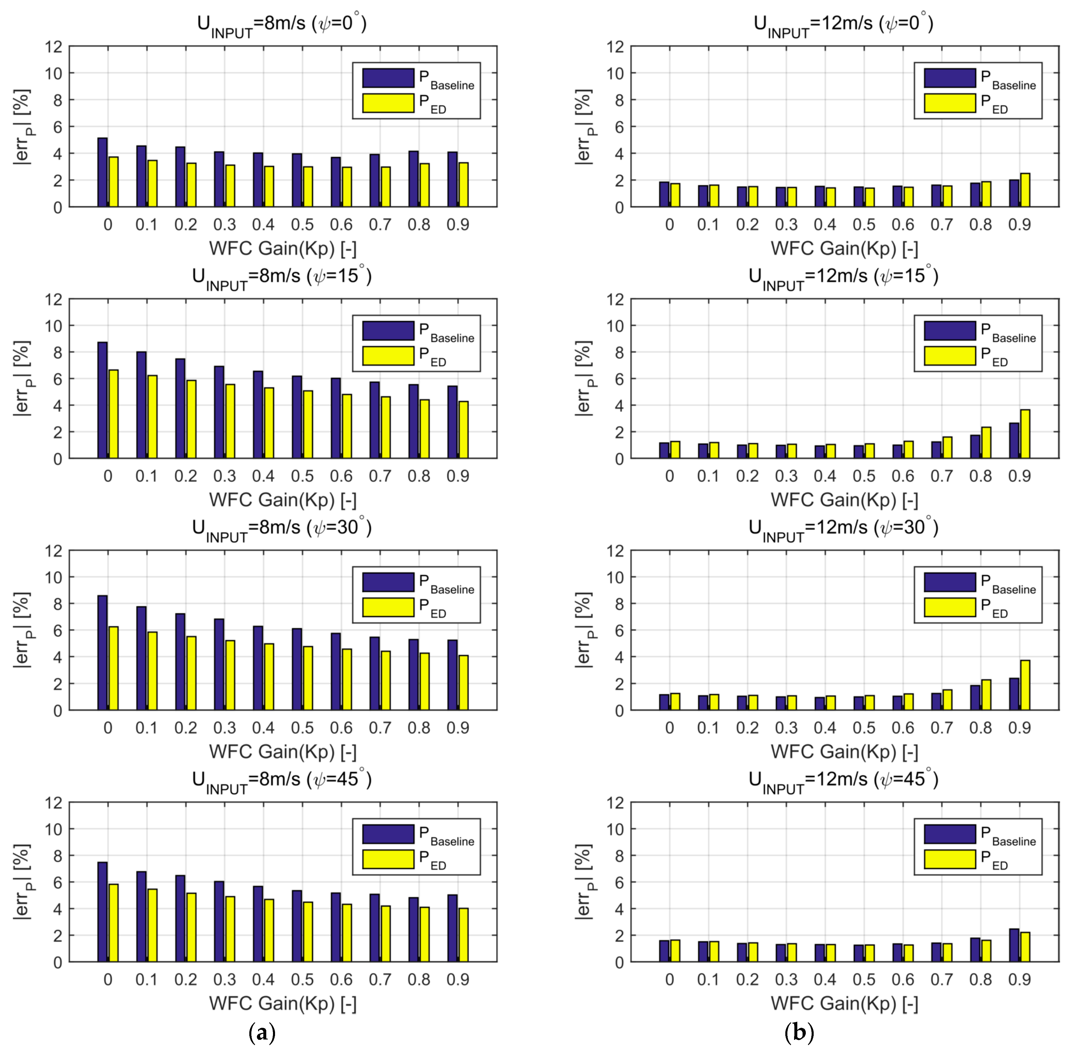
2.3.2. Wind Farm Simulation

In this study, the scenarios were designed by combining various wind speeds and directions, as introduced in Section 2.1, and the wind farm control gain, Kp. Control gain of the wind farm controller was applied to all scenarios composed of a combination of wind speed and wind direction. This study confirmed that the wind farm’s power output and tower load of each wind turbines varied according to changes in control gain throughout the simulation. The wind speeds considered in this study were 8 m/s below the rated wind speed and 12 m/s above the rated wind speed. The wind speed data used in the simulation were turbulent winds with a turbulence intensity of 0.09 generated based on Veer’s model.

In this study, the performance of the closed-loop wind farm controller was confirmed through this configuration. Figure 8 shows an example of the results from the simulation. The conditions applied to the simulation were a $U_{INPUT}$ of 12 m/s and a $U_{DIR}$ of 0 degrees. The power command distribution method applied to the power plant controller was proportional allocation.

Figure 8a shows the change in the power command of TSO and the change in the power output of the wind farm over the time domain. As described above, the power command of the TSO was fixed at 100 MW because it represented the number of wind turbines multiplied by the rated power for 300 s. However, since it was set to be approximately 80% of the average available power 300 s from the start of the simulation, the power command was reduced.

Figure 8b shows the power command and the power output in the time domain accordingly. As shown in Figure 8b, since each wind farm is required higher than the available power output before 300 s, the power command distributed to the individual wind turbine is higher than the available power. However, since the TSO power command was reduced to 80% of available power after 300 s, the required power output for each wind turbine was also reduced. The wind turbine that receives the reduced power command reduces the error between the input power command and the actual power output using the DPPT algorithm installed in the controller.

Figure 8c shows the thrust force of each wind turbine in the time domain. As shown in the figure, upstream wind turbines experience higher thrust forces than downstream ones. However, because the power command was reduced after 300 s, the power output of the upstream wind turbines was regulated and the tower load was reduced.

Since all the simulation results were derived from the same time domain, it is not suitable for directly comparing changes in wind direction and power output. Therefore, in this study, the representative values calculated by Equations (18) and (19) for power output and the tower load, respectively, were used to compare the control performance of the wind farm. To compare the tower load, the damage equivalence load (DEL) was used and only the tower loads of wind turbines 1–5 were compared. The numbers assigned to the turbines is shown in Figure 2.

$$er{r}_P=\frac{1}{T}{\displaystyle {\int }_0^T\frac{{\displaystyle \sum _{i=1}^N{P}_i}(t)-TS{O}_{CMD}(t)}{TS{O}_{CMD}(t)}dt}$$

(18)

where N is number of wind turbine and T is simulation time.

$$DEL={\left(\frac{{\displaystyle \sum _k{n}_k{S}_k^m}}{N_{eq}}\right)}^{\frac{1}{m}}$$

(19)

In Equation (19), $S_k$ is the stress of the tower load with kth magnitude of the total tower load during a specified evaluation (simulation) time (commonly 600 s), $n_k$ is the number of cycles of $S_k$, and $N_{eq}$ is the equivalent number of cycles of DEL (which is commonly calculated from the evaluation (simulation) time multiplied by a frequency of 1 Hz). In Equation (19), m is a constant related to the slope of the SN (stress to cycles to failure) curve of a material. For a steel tower, a value of 3.5 was used for m [38].

3. Discussion

Figure 9 shows the mean absolute error of total power output over the TSO power command versus different wind speeds, directions, and controller gains. Figure 9a shows the result of the input wind speed is below rated wind speed and Figure 9b shows the input wind speed is above rated wind speed.

In the graph, the x-axis represents the controller gain, Kp, applied to the wind farm controller, and the y-axis represents the error calculated by Equation (17).

In the figure, $P_{Baseline}$ was the result obtained when the proportional distribution model was applied to the wind farm controller, while $P_{ED}$ was the result obtained when the equal distribution model was applied. As shown in the figure, this study confirmed that it is effective to reduce the power output error compared to the TSO power command when the wind farm controller is composed of a closed-loop, irrespective of changes in the wind speed or direction. In particular, the method of distributing the power command equally to each wind turbine is an effective control method in terms of the accuracy and stability of wind farm power output and the reduction of upstream wind turbine DEL when the power command of TSO is lower than the wind farm’s available power.

In addition, the simulation results show that the change of the Kp due to the change in wind direction is remarkable. When the input wind speed was lower than the rated wind speed, Kp was effective in the range of 0.4 to 0.6 when the wind turbine distance was relatively close due to the wind direction changes. However, when the distance between the wind turbines increases due to a change in the wind direction change, the wind farm control effect can be increased only by increasing the controller gain. However, when the input wind speed was higher than the rated wind speed, different results were obtained. When the wind speed input to the wind farm was higher than the rated wind speed, Kp, which was set relatively high, the power generation error increased more than in the open-loop-based wind farm controller. In other words, the Kp of the wind farm controller is inversely proportional to the time taken for the wake to move to the downstream turbine.

Figure 10 shows the wind turbine power command distribution method and the standard deviation of power output according to the change in the wind farm controller Kp. As shown in the figure, when the equal distribution model was applied to the wind farm controller it was effective in securing the stability of the entire power output of the wind farm. Figure 10a shows the result of the input wind speed is below rated wind speed and Figure 10b shows the input wind speed is above rated wind speed.

The equal distribution model distributes power commands considering only the power command changes of the TSO regardless of the available power due to the state changes of the individual wind turbine, as introduced in Section 2.2.

Of course, this distribution scheme exhibits less effective performance than the proportional distribution model in terms of power output accuracy and stability at the moment of change in the TSO power command, as shown in Figure 8. However, greater output accuracy and stability can be secured compared to the proportional distribution model when the wind farm controller with closed-loop was maintained for a few minutes with lower available power than the TSO power command. However, when the wind speed was higher than the rated wind speed, that is, when the wake caused by the operational change of the upstream wind turbine was rapidly transferred to the downstream wind turbine, the higher set Kp served as a factor to reduce the performance of the equal distribution model.

Figure 11 shows the change in the power command of TSO and the change in the power output of the wind farm over the time domain. As described above, the power command of the TSO was fixed at 100 MW because it represented the number of wind turbines multiplied by the rated power for 300 s. However, since it was set to be approximately 80% of the average available power 300 s from the start of the simulation, the power command was reduced.

Figure 12 shows the results of comparing the power command distribution method and tower load change according to the wind farm controller Kp gain change based on the wind speed change. Figure 12a shows the result of the input wind speed is below rated wind speed and Figure 12b shows the input wind speed is above rated wind speed.

The simulation code used in this study basically uses the wind turbine model based on the BEM theory and the wake model based on the parabolic Reynolds-averaged Navier–Stokes. Thus, it was impossible to implement the tip vortex generated by the blade tip. Therefore, the tower load comparison due to the partial wake could not be conducted accurately, and as a result, the tower load comparison in this study was performed only at 0 degrees. The calculated DEL for each condition is shown in Figure 12.

First, when the wind speed input to the wind farm was lower than the rated wind speed, the DEL of the upstream wind turbine was ~26% smaller when the equal distribution model was applied to the wind farm controller than when the proportional distribution model was applied. Also, when the input wind speed was higher than the rated wind speed, the DEL was ~17% smaller.

The magnitude of DEL is proportional to the magnitude and frequency of the tower load, as introduced by Equation (19), and is most influenced by the magnitude of the tower load. Unlike the proportional distribution model, the equal distribution model assumes that the same power output can be obtained from the downstream wind turbines and distributes the power command, thus reducing the power output duty of the upstream wind turbines. For this reason, the equal distribution model has the effect of letting the wind flow more freely downstream, reducing the DEL of the upstream wind turbines.

Simulation has confirmed that the equal distribution model can reduce the DEL of upstream wind turbines, but there is no significant change in the DEL of downstream wind turbines due to the small variation in the output command and the increased turbulence intensity.

4. Conclusions

In this study, the performance of the proposed wind farm controller composed of a closed-loop was verified using an in-house wind farm simulation code. The wind farm was modeled by using 20 NREL 5 MW wind turbines with a distance between the turbines set to six times the rotor rotation diameter in both lateral and longitudinal directions. The performance of the wind farm controller was evaluated by comparing the power error, deviation, and tower load of each wind turbines according to Kp variation based on different wind speeds and directions. Also, the TSO power command was set to be lower than the available power and both the proportional distribution model and equal distribution model were applied to the wind farm controller.

This study confirmed that the equal distribution model is more effective in terms of wind farm power output accuracy, stability, and tower load than the proportional distribution model when the structure of the wind farm controller is closed-loop. In particular, the tower load on the upstream wind turbines, which experienced the greatest load, was reduced regardless of changes in wind speed and direction. This result was due to the fact that the equal distribution model simply distributes the output without any estimate, unlike the proportional distribution model, which distributes the power command based on the estimated wind speed.

The wake generated by the wind turbine increases the wind speed through the mixing process with the surrounding atmospheric wind as the distance in the downstream direction increases. However, even if the wind speed is the same, if the distance required for wake recovery is increased due to the wind direction change, Kp must be reduced inversely to confirm that the performance of the wind farm controller is maintained by simulation. Also, if the kinetic energy of the wind is higher than the allowable energy of the wind turbine, the wind speed is recovered rapidly because the wake strength is weakened. Therefore, the simulation shows that the performance of the wind farm controller was improved as Kp is smaller. In other words, the simulation shows that the feedback gain of the wind farm controller is inversely proportional to the wake recovery rate. For this reason, the control gain must be adjusted according to environmental changes through gain scheduling to improve the efficiency of the wind farm. Therefore, altering gain scheduling according to changes in the surrounding environment is a key area for future research.

References

1. GWEC. Global Wind Report Annual Market Update 2017; Global Wind Energy Council: Brussels, Belgium, 2018. [Google Scholar]
2. IRENA. Renewable Power Generation Costs in 2017; International Renewable Energy Agency: Abu Dhabi, UAE, 2018. [Google Scholar]
3. Chowdhury, S.; Zhang, J.; Messac, A.; Castillo, L. Unrestricted wind farm layout optimization (UWFLO): Investigating key factors influencing the maximum power generation. Renew. Energy 2012, 38, 16–30. [Google Scholar] [CrossRef]
4. Fleming, P.A.; Ning, A.; Gebraad, P.M.O.; Dykes, K. Wind plant system engineering through optimization of layout and yaw control. Wind Energy 2016, 19, 329–344. [Google Scholar] [CrossRef]
5. Shakoor, R.; Hassan, M.Y.; Raheem, A.; Wu, Y. Wake effect modeling: A review of wind farm layout optimization using Jensen’s model. Renew. Sustain. Energy Rev. 2016, 58, 1048–1059. [Google Scholar] [CrossRef]
6. Gustave, P.C.; Pieter, S. Heat and flux: Increase of wind farm production by reduction of the axial induction. In Proceedings of the European Wind Energy Conference, Madrid, Spain, 16–19 June 2003. [Google Scholar]
7. Corten, G.P.; Schaak, P. More power and less loads in wind farms. In Proceedings of the European Wind Energy Conference, London, UK, 22–25 November 2004. [Google Scholar]
8. Machielse, L.A.H.; Barth, S.; Bot, E.T.G.; Hendriks, H.B.; Schepers, G.J. Evaluation of ‘Heat and Flux’ Farm Control; Technical Report ECN-E–07-105; Energy Research Centre of the Netherlands: Sint Maartensvlotbrug, The Netherlands, 2007. [Google Scholar]
9. Kim, H.; Kim, K.; Paek, I. Power regulation of upstream wind turbines for power increase in a wind farm. Int. J. Precis. Eng. Manuf. 2016, 17, 665–670. [Google Scholar] [CrossRef]
10. Kim, H.; Kim, K.; Paek, I. Model based open-loop wind farm control using active power for power increase and load reduction. Appl. Sci. 2017, 7, 1068. [Google Scholar] [CrossRef]
11. Fleming, P.A.; Gebraad, P.M.; Lee, S.; van Wingerden, J.W.; Johnson, K.; Churchfield, M.; Michalakes, J.; Spalart, P.; Moriarty, P. Evaluating techniques for redirecting turbine wakes using SOWFA. Renew. Energy 2014, 70, 211–218. [Google Scholar] [CrossRef]
12. Gebraad, P.; Teeuwisse, F.; Wingerden, J.; Fleming, P.A.; Ruben, S.; Marden, J.; Pao, L. Wind plant power optimization through yaw control using a parametric model for wake effects—A CFD simulation study. Wind Energy 2016, 19, 95–114. [Google Scholar] [CrossRef]
13. Quick, J.; Annoni, J.; King, R.; Dykes, K.; Fleming, P.; Ning, A. Optimization under Uncertainty for Wake Steering Strategies. J. Phys. Conf. Ser. 2017, 854, 012036. [Google Scholar] [CrossRef]
14. Fleming, P.; Annon, J.; Shah, J.J.; Wang, L.; Ananthan, S.; Zhang, Z.; Hutchings, K.; Wang, P.; Chen, W.; Chen, L. Field test of wake steering at an offshore wind farm. Wind Energy Sci. 2017, 2, 229–239. [Google Scholar] [CrossRef] [Green Version]
15. Raach, S.; Boersma, S.; van Wingerden, J.; Schlipf, D.; Cheng, P.W. Robust lidar-based closed-loop wake redirection for wind farm control. IFAC-PapersOnLine 2017, 50, 4498–4503. [Google Scholar] [CrossRef]
16. Kanev, S.; Savenije, F.; Soleimanzadeh, M.; Wiggelinkhulzen, E. Wind Farm Modeling and Control: Inventory; ECN Technical Report; ECN-E-13-058; Energy Research Centre of the Netherlands: Sint Maartensvlotbrug, The Netherlands, 2013. [Google Scholar]
17. Ketterer, J.C. The impact of wind power generation on the electricity price in Germany. Energy Econ. 2014, 44, 270–280. [Google Scholar] [CrossRef] [Green Version]
18. Kristoffersen, J.R.; Christiansen, P. Horns Rev offshore wind-farm: Its main controller and remote control system. Wind Eng. 2003, 27, 351–359. [Google Scholar] [CrossRef]
19. Zhao, H.; Wu, Q.; Guo, Q.; Sun, H.; Xue, Y. Distributed model predictive control of a wind farm for optimal active power control Part II: Implementation with clustering based piece-wise affine wind turbine model. IEEE Trans. Sustain. Energy 2015, 6, 840–849. [Google Scholar] [CrossRef]
20. Zhao, H.; Wu, Q.; Huang, S.; Shahidehpour, M.; Guo, Q.; Sun, H. Fatigue load sensitivity-based optimal active power dispatch for wind farms. IEEE Trans. Sustain. Energy 2017, 8, 1247–1259. [Google Scholar] [CrossRef]
21. Zhang, J.; Liu, Y.; Tian, D.; Yan, J. Optimal power dispatch in wind farm based on reduced blade damage and generator losses. Renew. Sustain. Energy Rev. 2015, 44, 64–77. [Google Scholar] [CrossRef]
22. Guo, Y.; Gao, H.; Wu, Q.; Østergaard, J.; Yu, D.; Shahidehpour, M. Distributed coordinated active and reactive power control of wind farms based on model predictive control. Electr. Power Energy Syst. 2019, 104, 78–88. [Google Scholar] [CrossRef] [Green Version]
23. Boersma, S.; Doekemeijer, B.M.; Siniscalchi-Minna, S.; van Wingerden, J.W. A constrained wind farm controller providing secondary frequency regulation: An LES Study. Renew. Energy 2019, 134, 639–652. [Google Scholar] [CrossRef]
24. Jacob, D.G.; Soltani, M.N.; Torben, K.; Martin, N.K.; Thomas, B. Aeolus toolbox for dynamics wind farm model, simulation and control. In Proceedings of the European Wind Energy Conference and Exhibition (EWEC) 2010, Warsaw, Poland, 20–23 April 2010; European Wind Energy Association (EWEA): Warsaw, Poland, 2010. [Google Scholar]
25. Kim, H.; Kim, K.; Paek, I.; Yoo, N. Development of a time-domain simulation tool for offshore wind farms. J. Power Electron. 2015, 15, 1047–1053. [Google Scholar] [CrossRef]
26. Kim, H.; Kim, K.; Bottasso, C.L.; Campagnolo, F.; Paek, I. Wind turbine wake characterization for improvement of the Ainslie eddy viscosity wake model. Energies 2018, 11, 2823. [Google Scholar] [CrossRef]
27. Kim, K.; Kim, H.; Kim, C.; Paek, I.; Bottasso, C.L.; Campagnolo, F. Design and validation of demanded power point tracking control algorithm of wind turbine. Int. J. Precis. Eng. Manuf. Green Technol. 2018, 5, 387–400. [Google Scholar] [CrossRef]
28. Ainslie, J.F. Calculating the flowfield in the wake of wind turbine. J. Wind Eng. Ind. Aerodyn. 1988, 27, 213–224. [Google Scholar]
29. Jiménez, A.; Crespo, A.; Migoya, E. Application of a LES technique to characterize the wake deflection of a wind turbine in yaw. Wind Energy 2010, 13, 559–572. [Google Scholar] [CrossRef]
30. Gebraad, P.M.O.; van Wingerden, J.W. Maximum power-point tracking control for wind farms. Wind Energy 2015, 18, 429–447. [Google Scholar] [CrossRef]
31. Per, N.; Jens, V.; Jon, K.; Per, M.; Thomas, J.; Morten, L.T.; Mads, V.S.; Thoas, S.; Lasse, S.; Mauricio, M.; et al. WindPRO User Guide; EMD International A/S: Aalborg, Denmark, 2012. [Google Scholar]
32. Jonkman, J.; Butterfield, S.; Musial, W.; Scott, G. Definition of a 5-MW Reference Wind Turbine for Offshore System Development; Technical Report NREL/TP-500-38060; National Renewable Energy Laboratory: Golden, CO, USA, 2009.
33. 4C Offshore. 2014. Available online: www.4coffshore.com/windfarms (accessed on 4 January 2018).
34. Kim, K.; Lim, C.; Oh, Y.; Kwon, I.; Yoo, N.; Paek, I. Time-domain dynamic simulation of a wind turbine including yaw motion for power prediction. Int. J. Precis. Eng. Manuf. 2015, 15, 2199–2203. [Google Scholar]
35. Singh, M.; Santoso, S. Dynamic Models for Wind Turbines and Wind Power Plants; Subcontract Report NREL/SR-5500-52780; National Renewable Energy Laboratory: Golden, CO, USA, 2011.
36. Hansen, A.D.; Sørensen, P.; Iov, F.; Blaabjerg, F. Centralised power control of wind farm with doubly fed induction generators. Renew. Energy 2006, 31, 935–951. [Google Scholar]
37. Guan, X.; Molen, G.M. Aeolus Project Deliverable d3.1: Control Strategy Review and Specification (Part 1); Technical Report; Industrial Systems and Control, Applied Control Technology Consortium, Industrial Systems and Control Ltd.: Glasgow, Scotland, 2009. [Google Scholar]
38. Nam, Y. Wind Turbine System Control, 1st ed.; GS Intervision: Seoul, Korea, 2013; pp. 400–401. [Google Scholar]
Figure 1. Structure of the wind farm in-house simulation code.
Energies 12 02004 g001
Figure 2. Schematic of the wind turbine model.
Energies 12 02004 g002
Figure 3. Wind farm layout with different wind directions.
Energies 12 02004 g003
Figure 4. The wind turbine power curve and thrust coefficient variation according to wind speed changes: (a) wind turbine power curve and (b) thrust coefficient curve.
Energies 12 02004 g004
Figure 5. The wind farm layout for wind farm simulation code validation.
Energies 12 02004 g005
Figure 6. Schematic of the wind farm controller.
Energies 12 02004 g006
Figure 7. Comparison electrical power variation in time domain between measured data and simulation data.
Energies 12 02004 g007
Figure 8. Example of the time domain simulation results: (a) electrical power variation of wind farm and transmission system operator (TSO) command in time domain, (b) electrical power variation of each wind turbine and power command in time domain, and (c) thrust force variation of each wind turbine in time domain.
Energies 12 02004 g008
Figure 9. The comparison of power output error between open-loop and closed-loop with Kp variation: (a) below rated wind speed case and (b) above wind speed case.
Energies 12 02004 g009
Figure 10. Comparison of the standard deviation of total power output between open-loop and closed-loop with Kp variation: (a) below rated wind speed case and (b) above wind speed case.
Energies 12 02004 g010
Figure 11. Transient region in power output with TSO command change.
Energies 12 02004 g011
Figure 12. Comparison of damage equivalent load between open-loop and closed-loop with Kp variation: (a) below rated wind speed case and (b) above wind speed case.
Energies 12 02004 g012