Quantitative Evaluation of the “Non-Enclosed” Microseismic Array: A Case Study in a Deeply Buried Twin-Tube Tunnel

Abstract

The high-stress hazards of underground engineering have stimulated the exploration of microseismic monitoring and early warning methods. To achieve a good monitoring effect, the monitoring object is usually enclosed by a microseismic array (sensor array) (e.g., slope engineering, etc.). However, some characteristics of a buried tunnel, including “linear”, “deep-buried”, and “long”, make it difficult to deploy a reasonable microseismic array, which leads to the microseismic array being non-enclosed for the monitoring object. Application of the non-enclosed microseismic array yields decreases the accuracy of the source location. To solve the problem wisely, this paper deals with the feasibility of non-enclosed microseismic arrays (axial-extended, lateral-extended, and twin-tube arrays) by introducing a quantitative method. To this end, an optimized microseismic array with the best source location accuracy for a twin-tube expressway tunnel is proposed. The obtained results reveal that the non-enclosed microseismic arrays, which are unavoidable in expressway tunnel engineering, do not introduce errors but reduce the ability to resist them. Further, the twin-tube array achieves a better source location accuracy than the axial and lateral-extended arrays. In the application of the source location based on the particle swarm optimization (PSO) algorithm to the twin-tube array, microseismic events, which cluster in the rockburst section, are wholly gathered, and the maximum error is reduced by about 30–50 m, indicating its greater feasibility with respect to the single-tube array.

1. Introduction

Because of the unique topography and complicated geological conditions prevalent in Western China, the construction of tunnels and other underground projects is complicated. Tunnel engineering is a kind of linear distribution engineering, which has the characteristics of long-distance and large-buried depth. Due to the complex geological conditions and particularities of tunnel engineering, geological disasters frequently occur in tunnels, leading to the rapid development of microseismic monitoring technology and early-warning methods for disasters. As an advanced spatial 3D technology, microseismic monitoring has been widely exploited in the transportation field, hydropower projects, and the extraction and storage of various types of energy, such as mining engineering, slope engineering, underground and tunnel engineering, shale-gas exploitation, and hot dry rock reservoirs [1,2,3,4,5,6]. The ability to accurately trace microseismic events can be employed to judge the process by which fracture networks develop within rock masses [7,8,9]. Combining seismological theory with the analysis of various seismic data (such as seismic deformation, stress adjustment, energy release, etc.) of rock mass deformation and failure process, the activity law of potential disasters could be determined, and early warning could be possible to achieve dynamic analysis, control rock mass stability, and protect staff and equipment [10,11,12].

However, the accuracy of locating the source of microseismic events in deep-buried tunnel engineering cannot be guaranteed for the following reasons: (1) engineering activities in deep-buried tunnels where the drill-and-blasting method is used inevitably yield strong dynamic disturbances and thereby, generate a large number of microseismic events around the area of the tunnel face. Unlike traditional microseismic monitoring in the coal mining industry as well as industries pertinent to oil and coal seam gas explorations, microseismic arrays in deep-buried tunnels cannot form an optimal spatial distribution to fully cover microseismic events due to the highly limited amount of underground space. Hence, the accuracy with which the source is located is compromised or even unreliable; (2) the propagation of seismic waves is significantly affected by the excavated part of the tunnel, which physically represents a void area that may distort the shapes of the seismic signals. Further, the high-frequency components of the signal might be deflected and attenuated at the tunnel wall, and fracture zones and other underground structures make the constant velocity model unsuitable for locating the sources of microseismic events.

The use of a non-enclosed array is generally difficult to avoid in deep-buried tunnel engineering. To handle this problem, tri-axial sensors and corresponding source location methods have been proposed to break the limits from the non-enclosed array [13,14,15,16,17]. The effectiveness of the tri-axial method is also limited due to the near-field characteristics of microseismic events in tunnel engineering as well as the difficulty of distinguishing between P-waves and S-waves in acquisition channels. Therefore, some studies of microseismic arrays in deep-buried tunnels have been conducted to solve the problem [18,19]. However, quantitative evaluations of the layout of a sensor array in deep-buried tunnels have rarely been discussed in previous studies and have mainly involved coal mine and laboratory tests [20,21,22]. Consequently, an optimized microseismic array for a deep-buried, twin-tube expressway tunnel must be proposed to deal with a large number of engineering projects.

Herein, we discuss the layouts of non-enclosed microseismic arrays in deep-buried tunnels and the accuracy of their source locations is displayed by introducing a quantitative evaluation method based on the residual calculation criterion. The main contributions of the present research can be summarized as follows: (1) an optimized microseismic array for twin-tube expressway tunnels is established to improve the limitations imposed by a non-enclosed microseismic array in deep-buried tunnel engineering; (2) because of the unsuitable constant velocity model, the particle swarm optimization (PSO) algorithm is employed to optimize source location and search for the multivariable equivalent velocity in the Micang Mountain tunnel on the Bashan Expressway. The related methods and results are expected to provide a reference for the microseismic monitoring of deep-buried twin-tube tunnels to obtain a more accurate source location and to achieve effective monitoring and warnings concerning potential hazards in tunnels.

2. Residual Analysis of the Non-Enclosed Microseismic Array

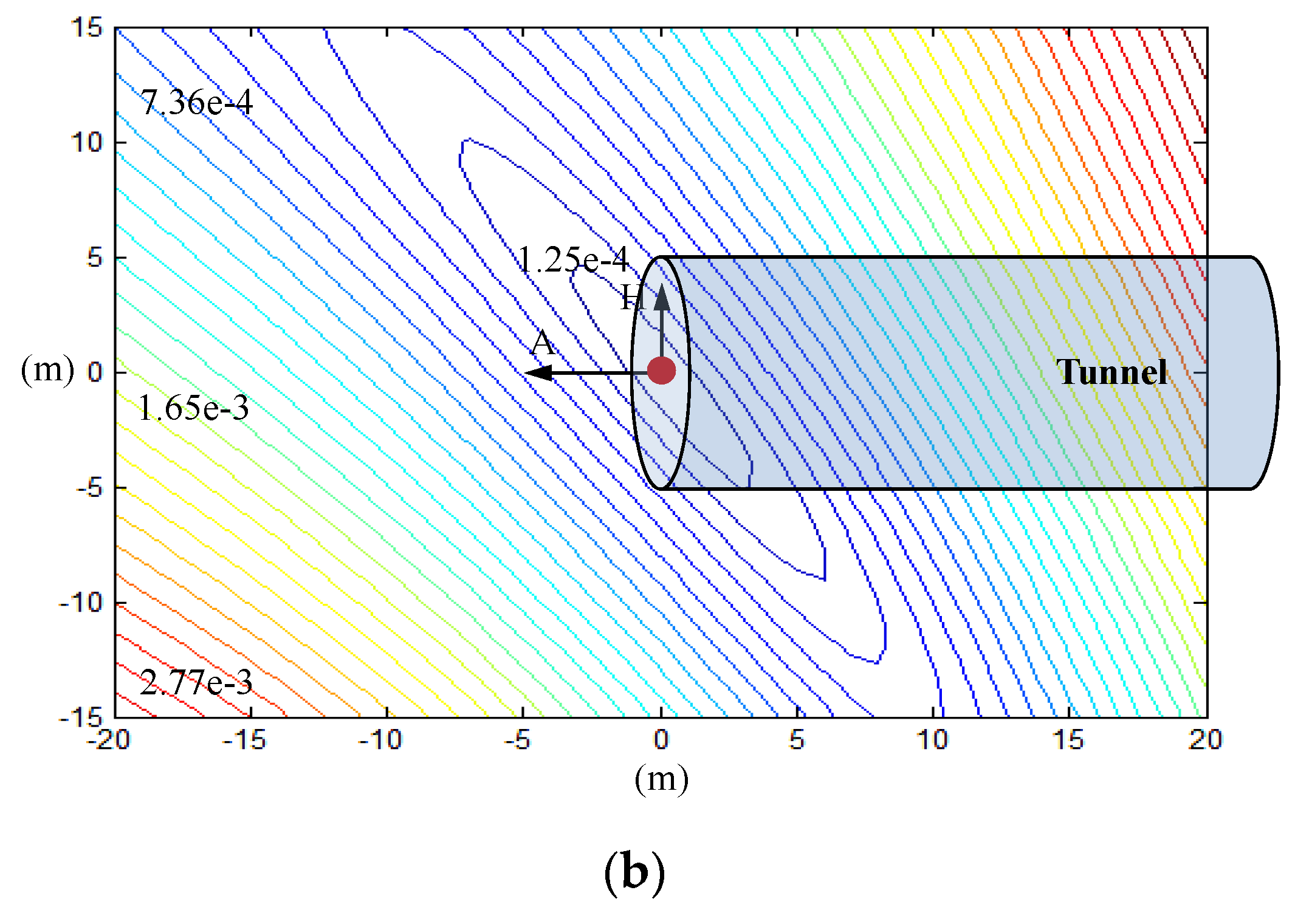
2.1. Introduction of Residual Criterion

Ideally, a source location error refers to the difference between the actual location and the calculated location. In reality, however, the actual positions of microseismic events are generally not known. As a result, source location errors are mostly measured indirectly by some parameters related to their corresponding physical data [23]. Figure 1 shows the microseismic waveform signals received by a sensor array and the different sensors $T_i$ that pick up the observed arrival time $t_i$ of the microseismic wave.

During source location, the difference between the calculated and observed arrival times from a source position to the sensor is denoted by the residual error, $\gamma$, and the corresponding calculation method is provided as:

$$\gamma ={\displaystyle \sum }_{i=1}^n{\left(t_i^{p,s}-t_0-t_{ci}^{p,s}\right)}^m/n$$

(1)

where $n$ is the number of sensors in the array; $t_i$ and $t_{ci}$ are the observed arrival time and calculated travel time of sensor $i$, respectively; the superscripts $p$ and $s$ stand for the P wave and S wave, respectively; m is 1 or 2 and in order represents the norm statistical criteria L1 and L2; $t_0$ is the initial time of the source. $t_{ci}=R_i/v_i$, where $R_i$ is the distance between the source location $\left(x_0, y_0,z_0\right)$ and the sensor $\left(x_i, y_i,z_i\right)$, and $v_i$ is the velocity of the microseismic wave along the propagation path.

Mathematically, the number of effective microseismic sensors is usually greater than the source parameters; that is, the location process is a statically indeterminate problem, and the essence of source location is to find the point of the minimum residual value of a microseismic event in the monitoring space; this can be solved by the regression analysis method. To this end, the least squares method (L2 norm statistical criterion) and the least absolute value method (L1 norm statistical criterion) are the two most commonly used regression analysis methods.

Different residual error calculation criteria have different estimates for the initial time, $t_0$, of the source. For the L1 criterion, the initial time, $t_0$, is defined as the median of the difference between the observed arrival time and the calculated travel time (i.e., $t_0\{{\left(t_i-t_{ci}\right)\}}_{mid}$). For the L2 criterion, $t_0=\sum _{i=1}^n{t}_i/n-\sum _{i=1}^n{t}_{ci}/n$. Hence, the residuals of the L1 criterion $\left({\gamma }_1\right)$ and the L2 criterion $\left({\gamma }_2\right)$ are obtained by substituting $t_0$ into Equation (1) [24,25,26]:

$${\gamma }_1={\displaystyle \sum }_{i=1}^n\left|t_i-t_{ci}-\{\left(t_i-t_{ci}\right)\}{ }_{mid}\right|/n$$

(2a)

$${\gamma }_2=\sqrt{{\displaystyle \sum }_{i=1}^n{\left[\left(t_i-{\displaystyle \sum }_{i=1}^n\raisebox{1ex}{$t_i$}\!\left/ \!\raisebox{-1ex}{$n$}\right.\right)-\left(t_{ci}-{\displaystyle \sum }_{i=1}^n\raisebox{1ex}{$t_{ci}$}\!\left/ \!\raisebox{-1ex}{$n$}\right.\right)\right]}^2}/n$$

(2b)

The norm statistical criterion L1 takes the sum of the absolute values of the residuals of each station as the objective function and does not strengthen the function of the residuals of a single station in the calculation. In the process of source location, the influence of individual outliers on the calculation results can be effectively reduced, and when there are some large residual errors in the microseismic monitoring system, the location results will not be significantly changed. The major advantage of the norm statistical criterion L1 is that it has strong resistance to individual large errors and is more suitable for the location calculation of the microseismic source.

2.2. Irrationality of the Non-Enclosed Microseismic Array

The non-enclosed type of array is usually used in deep-buried tunnel engineering. To monitor the simulated microseismic event on the tunnel face (red sphere), a non-enclosed type array with three rows of monitoring sections is established, as demonstrated in Figure 2a. Each section has a spacing of 30 m, and the first section is at a distance of 40 m from the tunnel face. The sensors are located on the dome, the left, and the right sides of the wall, and $A$, $H$, and $V$ represent the axial, horizontal, and vertical directions of the tunnel, respectively. This non-enclosed type of array results in the residual contour density in the axial direction which is significantly lower than that in the horizontal direction, and the minimum residual range expands greatly in the axial direction, resulting in a “residual void.” In such a case, the error, $\Delta \gamma$, caused by an inaccurate pick-up arrival time and wave speed, will lead to a large displacement of the source position in the axial direction of the residual space. The same error value, $\Delta \gamma$, in different directions of the tunnel also causes different displacements, particularly in the axial direction (Figure 2b).

3. Evaluation and Optimization of Non-Enclosed Microseismic Arrays

3.1. Evaluation Method

An unreasonable sensor array layout leads to a reduction in the accuracy of the location. The $\gamma$ of the sensor $T_i$ in Equations (2a) and (2b) is now decomposed into three parts:

$${\gamma }_i=A_i-\left[B_i-C_i\right]$$

(3)

where $A_i$ is the difference between the pick-up arrival time of the sensor, and the average of that of the sensor array $(t_i-\sum _{i=1}^n{t}_i/n)$, $B_i$ is the calculated travel time $(t_{ci})$, $C_i$ is the average calculated travel time of the sensor array (i.e., $\left(\sum _{i=1}^n{t}_{ci}/n\right)$).

Assuming that the velocity of the waves in the microseismic monitoring space is uniform, $B_i$ is the distance from the source to the sensor, $T_i$, and $C_i$ is the distance from the source to the center of the sensor array, $T_0$. Therefore, $B_i-C_i$ constitutes the hyperbolic region, and it is equivalent to the difference between the distance from the source to the sensor, $T_i$, and the distance to the center, $T_0$, of the sensor array. Meanwhile, 2c represents the distance between $T_i$ and $T_0$, and $2a$ represents the distance difference from each point to $T_i$ and $T_0$. From the vertical bisection of the points $T_i$ and $T_0$ to the external extension line, the difference in the distance (i.e., $2a$) increases gradually from $0$ to $2c$. Then, the hyperbolic region is expressed as

$$\frac{x^2}{a^2}-\frac{y^2}{c^2-a^2}=1$$

(4)

Because of the characteristics of the non-enclosed array, the variation in the distance difference in the axial direction, $A$, of the tunnel has a small influence on the two outside points $T_i$ and $T_0$ of the hyperbolic domain. This corresponds to Equation (3) in which $\Delta \left(B_i-C_i\right)$ and $\Delta {\gamma }_i$ in the axial direction of the tunnel are smaller than the horizontal $H$, which explains the residual space effect in the axial direction, $A$, as shown in Figure 2b. We can improve the axial residual variation rate in the axial direction; for instance, $A_n,$ is significantly adjusted by adjusting the layout of the sensor array, as presented in Figure 3.

Although the residual variation rate in the horizontal direction, $H_n,$ is small at this time, it can be enhanced by adjusting the relationship between the center of the sensor array, $T_0$, and the other sensors, $T_j$. Hence, the residual variation rates of $A_n$ and $H_n$ are large in the cross hyperbolic domain, as demonstrated in Figure 4.

To evaluate the control function of the sensor array on the accuracy of source location, the hyperbolic domain in a three-dimensional space is defined as follows:

$$\frac{x^2}{a^2}-\frac{y^2+z^2}{b^2}=1$$

(5)

The hyperbolic density, $d$, is the variation of the distance difference of the unit length in a direction. The greater the number of hyperbolic passes indicates the larger the difference in the distance. Thereby, the hyperbolic density on the $X$, $Y$, and $Z$ azimuth axes is obtained by the following relations [25]:

$$d_x=\frac{da}{dx}=xa/\left[\frac{a^4\left(y^2+z^2\right)}{c^2-a^2}+x^2\right]$$

(6)

$$d_y=\frac{da}{dy}=-y\left(c^2-a^2\right)/\left[\frac{x^2{\left(c^2-a^2\right)}^2}{a^3}+a\left(y^2+z^2\right)\right]$$

(7)

$$d_z=\frac{da}{dz}=-z\left(c^2-a^2\right)/\left[\frac{\left(x^2+z^2\right){\left(c^2-a^2\right)}^2}{a^3}+a{y}^2\right].$$

(8)

According to the angle between the tunnel azimuth and the coordinate axis, the hyperbolic density of the tunnel azimuth can be calculated by

$$d_d=\left|\frac{da}{dx}\right|{\cos }^2\alpha +\left|\frac{da}{dy}\right|{\cos }^2\beta +\left|\frac{da}{dz}\right|{\cos }^2\xi$$

(9)

where $\alpha$,$\beta$, and $\xi$ are the azimuth angles of the tunnel azimuth and the coordinate axis. Therefore, the total hyperbolic density (i.e., $\sum _{i=1}^n{d}_d/n$) can be obtained by evaluating the hyperbolic density of each sensor and the center of the sensor array. A large hyperbolic density represents the large residual variation rate, which is helpful for improving the accuracy of the source location. In practical applications for the linear distribution characteristics of tunnel engineering disasters, it is required that the accuracy of the location along the axial direction be better than that of the horizontal and vertical directions. As a result, to obtain a more reasonable sensor array for deep-buried tunnel engineering, the rationality of the residual space as well as the accuracy of the source location along the axial direction of the tunnel are discussed in the following sections.

3.2. Evaluation of Non-Enclosed Microseismic Arrays

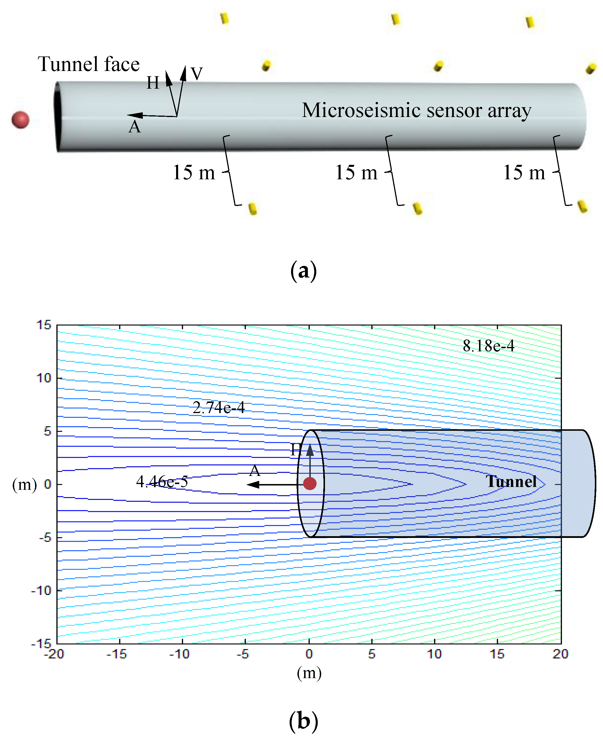
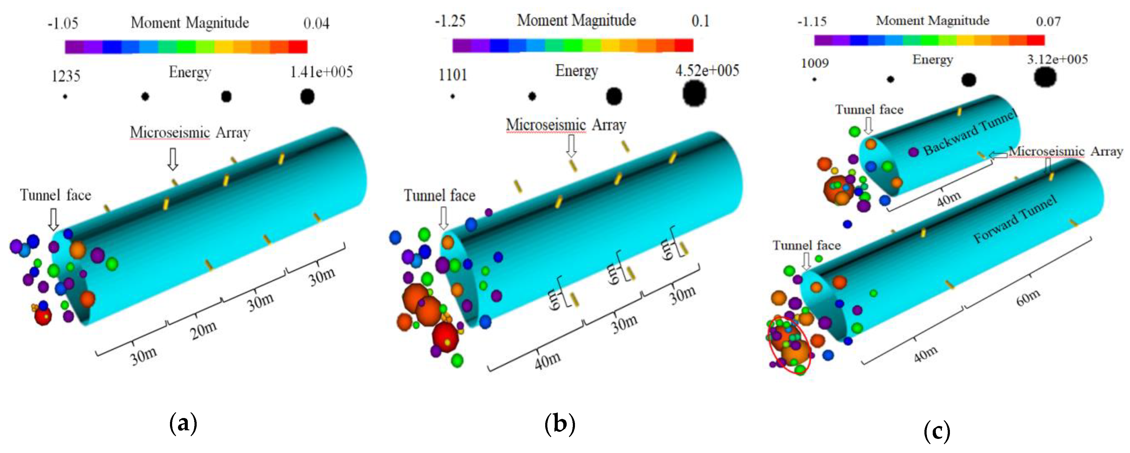
3.2.1. Axial-Extended Array

Based on the sensor array presented in Figure 2, the sensors on the left and right walls of each row are located at the front and back dislocations of 10 m, while the dome sensors remain unchanged. In this case, the residual space effect still exists, and the accuracy of locating the source has not been improved effectively. It implies that the search for other sensor arrays is highly needed.

3.2.2. Lateral-Extended Array

A lateral-extended sensor array is under investigation as schematically demonstrated in Figure 2, where the depths at which the buried sensors of each row are increased to 15 m (see Figure 5a). Compared with the axial-extended sensor array, the residual variation rate in every direction of the tunnel grows significantly, as the maximum value increases from 2.66 × 10⁻⁴ to 8.18 × 10⁻⁴ (see Figure 5b). Therefore, the lateral-extended sensor array enhances the source location accuracy.

The distribution curve of the hyperbolic density along the axial direction of the tunnel with the lateral-extended sensor array has been demonstrated in Figure 6, where the horizontal coordinates a–h correspond to the depths at which the sensors were buried (i.e., 3–24 m) at intervals of 3 m. Figure 6 shows that the hyperbolic density along the axial direction of the tunnel improved from 0.033 to 0.060 as the buried depth grew. However, burying the sensors at great depths is not a practical alternative in deep-buried tunnel engineering; thus, laterally-extended sensor arrays are slightly exploited in practice.

3.2.3. Twin-Tube Array

Twin-tube sensor arrays arranged in the forward and backward tunnels are commonly exploited to monitor microseismic events near the tunnel face of the backward tunnel, as presented in Figure 7. Using this array layout, the residual variation rate in every direction of the tunnel increases significantly to a maximum value of 2.77 × 10⁻³, and the residual space effect no longer exists in the axial direction, indicating that accuracy of the source location along the axial direction has been improved significantly. Furthermore, the sensor array in the backward tunnel extends the sensor array of the forward tunnel in the lateral orientation, which also improves the accuracy of the source location of the forward tunnel.

Also the distribution curve of hyperbolic density along the axial direction of the tunnel with the twin-tube sensor array is shown in Figure 6, where the horizontal coordinates a–h correspond to the positions of the array of sensors in the forward tunnel for the range of 0–70 m at intervals of 10 m. Figure 6 shows that with the sensor array position of the forward tunnel moving to the rear, the hyperbolic density along the axial direction of the tunnel decreased from 0.180 to 0.045. In actual twin-tube tunnel engineering, the layout of the sensor array (see Figure 7a) can be used to form an enclosed effect on the monitoring stage, which significantly improves the accuracy of the source location.

3.2.4. Non-Enclosed Microseismic Array Test

In order to further study the source location accuracy of different non-enclosed microseismic arrays, the artificial knock test was used, as shown in Figure 8. However, for lateral-extended arrays, this method has some limitations and sensor burial depths could only be extended to 6 m.

Table 1. Artificial knock test results. Knock points 1, 2, and 3 were located on the left wall, right wall, and vault of the same section of the tunnel, respectively. The table shows the experimentally measured and calculated coordinates of the knock points of the non-enclosed arrays.

		North (m)	East (m)	Depth (m)	Location Error Analysis (m)
Knock point 1	Actual measurement	850.23	982.33	1078.47	-
	Axial-extended array	845.21	969.13	1065.92	18.89
	Lateral-extended array	860.12	975.55	1090.19	16.77
	Twin-tube array	856.68	984.51	1085.21	9.58
Knock point 2	Actual measurement	858.69	996.91	1079.02	-
	Axial-extended array	867.58	982.31	1090.12	20.38
	Lateral-extended array	852.11	992.97	1068.21	19.28
	Twin-tube array	862.29	993.11	1085.96	8.69
Knock point 3	Actual measurement	854.48	990.04	1085.31	-
	Axial-extended array	850.34	998.25	1070.21	17.68
	Lateral-extended array	863.21	981.12	1095.55	16.14
	Twin-tube array	857.45	988.14	1091.78	7.37

shows the experimentally measured and calculated coordinates of the knock positions for different non-enclosed arrays. It was found that the location accuracy of the twin-tube array was better than those of the axial and lateral-extended arrays, and its location error was below 10 m which met the engineering requirements.

Based on the results obtained from the artificial knock test, the non-enclosed array was selected to monitor the ruptures in the surrounding rocks after tunnel excavation. A section of the tunnel with uniform geological conditions was selected as the test section and non-enclosed arrays were arranged in it. Stress adjustment was mainly concentrated around the excavation face which was the most prone to geological hazards. This way, the results obtained from non-enclosed arrays could be an indicative of the failures of the surrounding rocks near the tunnel excavation face. It could be clearly seen from the results that the concentration of microseismic events in the twin-tube array was higher than those of the axial and lateral-extended arrays, as shown in Figure 9. In summary, the location accuracy of the twin-tube array was the highest among non-enclosed arrays.

4. Optimization and Application of Microseismic Arrays for Twin-Tube Tunnels

4.1. Optimizing the Microseismic Array for a Twin-Tube Tunnel

A microseismic monitoring system is established and optimized in expressway twin-tube tunnel with the characteristics of “linear”, “deep-buried,” and “long”, as shown in Figure 10. It consisted of the following steps:

(1)

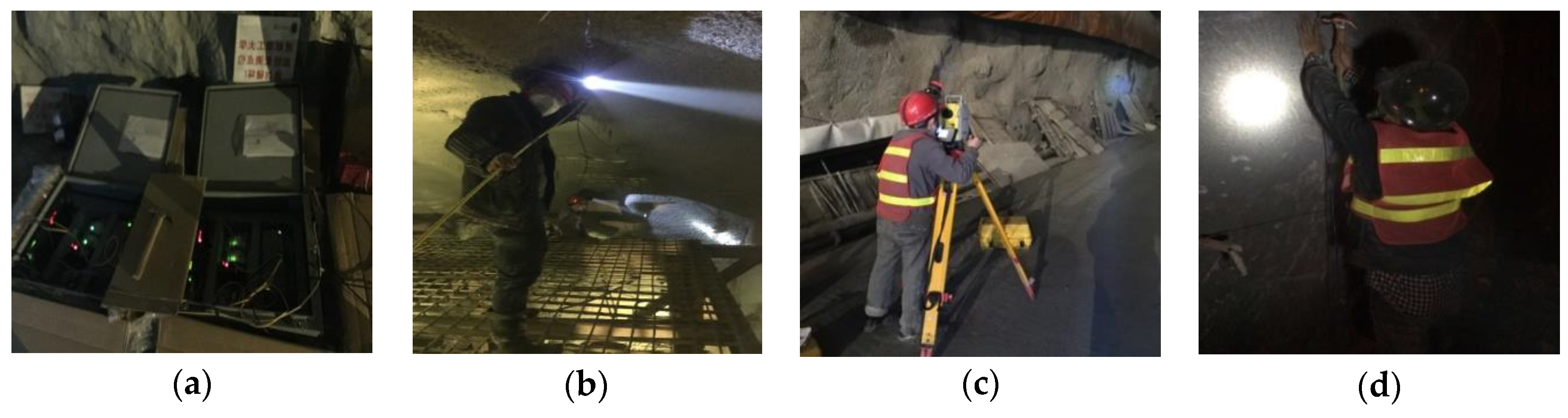
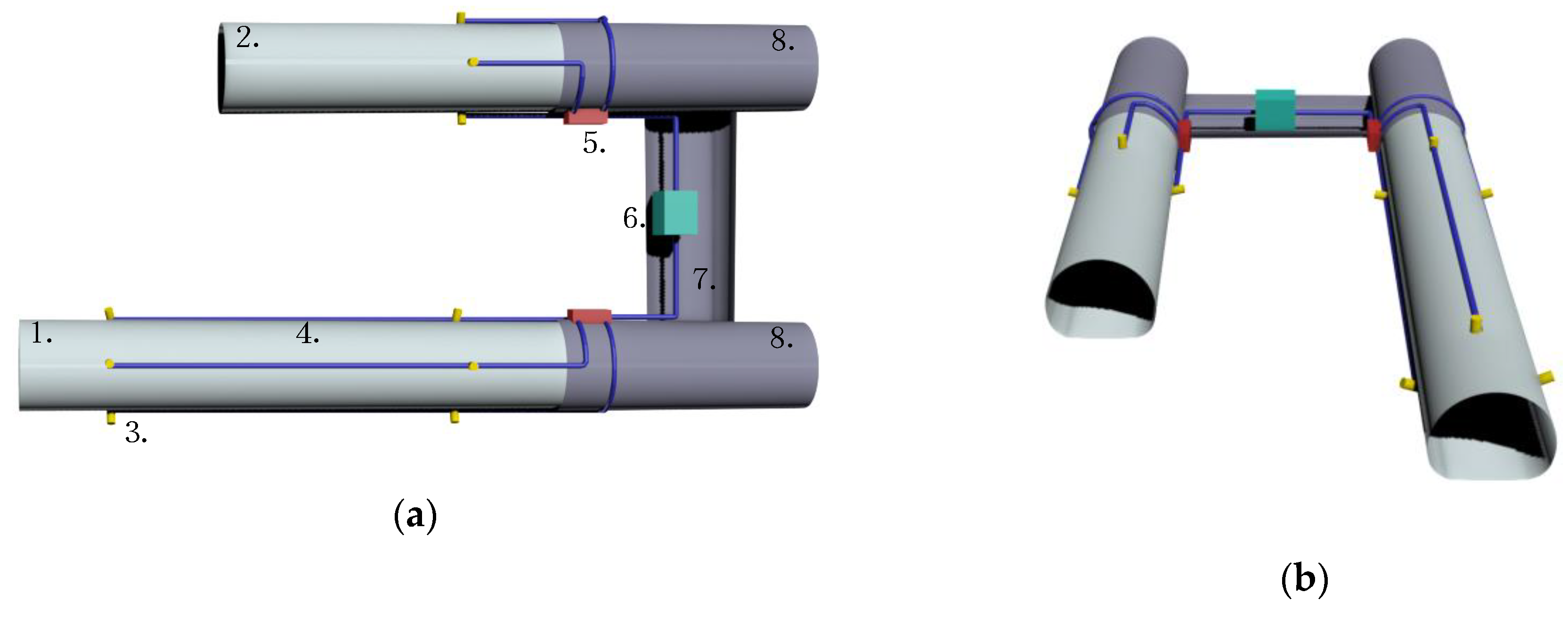
Due to the limited workforce, frequent traffic, and the interactions between various processes, the data acquisition station was placed in the rear of the secondary lining, and the data processing station was placed in the cross hole.

(2)

The twin-tube sensor array with three rows of monitoring sections was positioned in the twin-tube expressway tunnel with two rows of monitoring sections in the forward tunnel and one row in the backward tunnel. Each section had a spacing of 30–40 m, and the first section was 40–50 m from the tunnel face. The sensors were located on the dome and the left and right sides of the wall, and the sensors of each row were buried at depths of 3–4 m.

(3)

The cable between the sensor and the data acquisition station was suspended on the side wall of the tunnel by the pre-embedded expansion hook.

(4)

The sensor hole must be blocked by sound insulation cotton.

(5)

It was necessary to drill monitoring holes and install sensors according to the tunnel excavation.

(6)

The construction procedure of a tunnel excavation cycle involves drilling, blasting, slag, and vertical-arch grouting. The installation of the full-section sensor was mainly conducted by using the trolley in the slag-transport and shotcreting processes. In the drilling and standing-arch stage, an excavator or loader was used to remove the sensors at the higher positions on the side wall, and the dome sensor was removed by the vehicle after the secondary lining was followed up.

Among the above steps, step (3) greatly reduces interference and damage, and ensures a smooth monitoring process, step (4) is mainly to prevent the construction noise and the noise from the monitoring effect, and step (5) is to ensure the continuity of monitoring.

4.2. A Case Study

In this section, we describe the application of the optimized twin-tube array to practical engineering and use the PSO algorithm to search for multivariable equivalent velocity and the best source location. First of all, PSO is a new intelligent optimization method, which originated from a simulation of social behavior (the hunting behavior of birds). In such a method, the optimization approach updates the population of particles by applying an operator according to the fitness information obtained from the environment where the individuals of the population are expected to move towards a better solution. The calculation process of the PSO updates itself by tracking two extreme values: one is the optimal solution of the particle itself, and the other is the optimal solution of the entire population. Then, the updated equations of the velocity and location of the particles are as follows [27,28]:

$$v_i^{j+1}=\omega v_i^j+c_1\xi \left(p_i^j-x_i^j\right)+c_2\eta \left(p_g^j-x_i^j\right)$$

(10)

$$x_i^{j+1}=x_i^j+v_i^{j+1}$$

(11)

where $v_i$ and $x_i$ represent the velocity and location of the $i$-th particle, respectively; $\omega$ is the inertial weight for balancing the global and local searches; $c_1$ and $c_2$ are learning factors with positive constants; $\xi$ and $\eta$ are two random functions in the range of [0, 1]. $p_i$ and $p_g$ in order represent the best previous position of the $i$-th particle and the best previous position among all the particles in the search space. Referring to the above-mentioned PSO algorithm, the multivariable equivalent velocity is represented by $v_i$. For microseismic events in the left or right tunnels, the multivariable equivalent velocity $v_i$ denotes different meanings.

Figure 11 shows the twin-tube sensor array with three rows in the monitoring section that was installed in the Micang Mountain tunnel on the Bashan Expressway. Section 1, which contains two sensors, and Section 2, which contains three sensors, were located in the tunnel to the right of the advanced excavation, and Section 3, which contains three sensors, was located in the tunnel to the left of the delayed excavation. In this case, the sensor array shown in Figure 12 was able to distinguish the microseismic events that occurred on the tunnel face of the left tunnel or the right tunnel at the times of occurrence. It was possible to determine the position of the source by the arrival times of the microseismic waves in the twin-tube sensor array.

After initial judging of the position of the source from Figure 12, we had to determine the exact location of the microseismic event. For this purpose, a source location method based on PSO was established by using the residual error calculation criteria (Equation (2a)) as the objective function. Before using the MATLAB software to compute the PSO, the initial input parameters of the method with twin-tube microseismic array were set as follows [29]: the population size (number of candidate particles) was 1000; the inertia weight $\omega$ was 0.8; learning factors $c_1$ and $c_2$ were both 0.5; and the number of dimensions was six, including three coordinates ($X, Y, Z$) and three velocity models ($V_1,V_2,V_3$).

Table 2. Particle swarm optimization (PSO)-based source location method, including initial conditions setting and search results.

Initial Conditions
Sensor number	1-1	1-2	2-1	2-2	2-3	3-1	3-2	3-3
North (m)	868.37	861.8	835.38	841.91	845.61	860.14	862.84	866.82
East (m)	847.29	832.15	846.47	860.16	852.13	889.99	895.12	904.63
Depth (m)	1007.89	1007.91	1008.36	1008.56	1016.605	1009.62	1017.27	1009.66
Right hole event arrival time (s)	0.9517	0.9521	0.9584	0.9558	0.9558	0.9471	0.9474	0.9496
Left hole event arrival time (s)	0.4988	0.5027	0.5051	0.5002	0.5003	0.4907	0.4904	0.4882
PSO Search Results
Location	Event in the right tunnel				Event in the left tunnel
North (m)	950				910
East (m)	809				920
Depth (m)	1027				1001
V1 (m/s)	3570 (Corresponding sensor: 1-1, 1-2)				4337 (Corresponding sensor: 1-1, 2-2, 2-3)
V2 (m/s)	3747 (Corresponding sensor: 2-1, 2-2, 2-3)				4066 (Corresponding sensor: 1-2, 2-1)
V3 (m/s)	5395 (Corresponding sensor: 3-1, 3-2, 3-3)				5080 (Corresponding sensor: 3-1, 3-2, 3-3)

provides the corresponding initial conditions and the search results. The search samples were six-dimensional, including north, east, buried depth, and three wave velocities (i.e., V₁–V₃). In addition, the three wave velocities are corresponding to those of Section 1, Section 2, and Section 3, respectively, for the microseismic event in the right tunnel. They are also associated with the positive side with 1-1, 2-2, and 2-3 sensors; the dorsal side with 1-2 and 2-1 sensors; and Section 3, respectively, for the microseismic event in the left tunnel. Figure 13 and Figure 14 show the search processes for the PSO optimal samples and the optimal residual values. The results indicate that the optimal source position of the right tunnel was (950 m, 809 m, 1027 m) in front of the tunnel face, and that the optimal source of the left tunnel was (910 m, 920 m, 1001 m) on the right wall of the tunnel face.

Combined with the above-explained source location method, we discuss the distribution of microseismic events during rockburst in the Micang Mountain tunnel of the Bashan Expressway, as displayed in Figure 15. Compared with the source location of the single-hole sensor array and that of the twin-tube sensor array, the twin-tube sensor array had a better ability to resist errors and improve the accuracy of the source location, which shortened the error distance by 30–50 m. Also, this showed that the microseismic events occur in clusters in the rockburst area.

5. Conclusions

(1)

Microseismic arrays in expressway tunnel engineering with the characteristics of “linear”, “deep-buried,” and “long” are non-enclosed, which leads to a smaller variation in the residual error in each direction of the tunnel in the residual space, especially in the axial direction, and produces a residual space effect. The non-enclosed microseismic array reduces the source location accuracy and the ability to resist external interferences or errors.

(2)

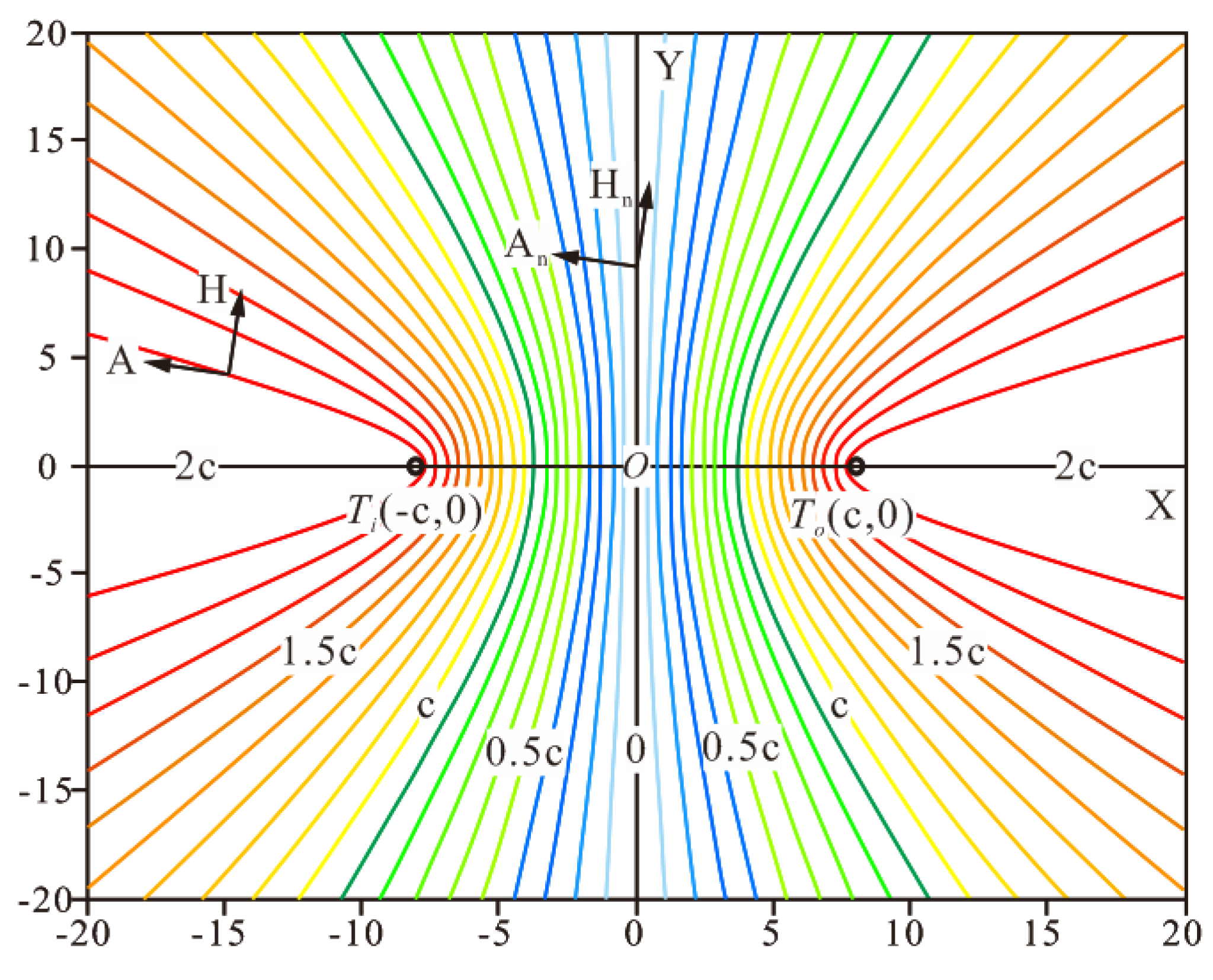
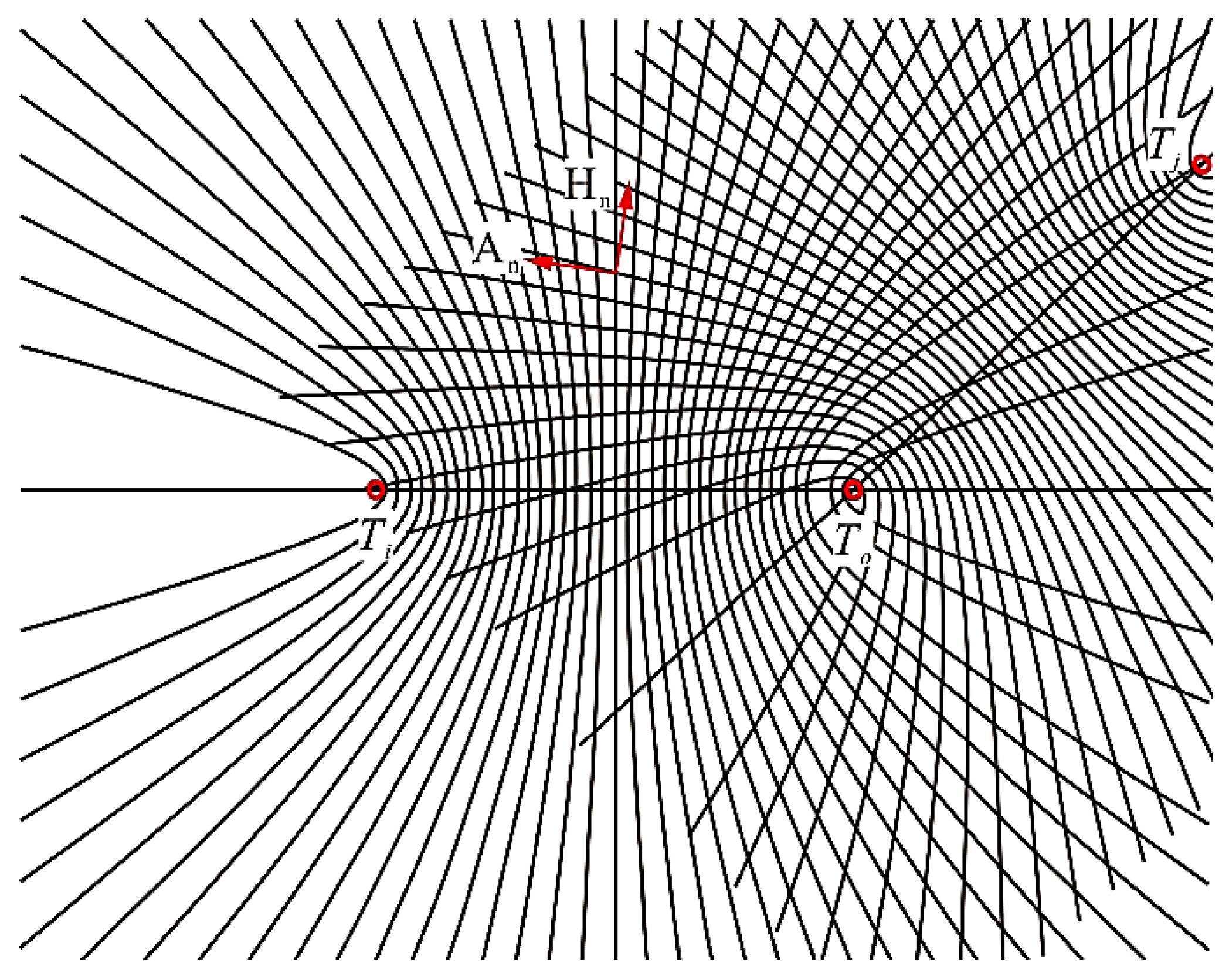
Based on the residual criterion and the residual composition of the source location, the residual variation was equivalent to the hyperbolic domain of the source distance difference. The effectiveness of the sensor array in controlling the accuracy of the location along each direction of the tunnel was evaluated by introducing the hyperbolic density index (i.e., a method to obtain a quantitative evaluation of the sensor array).

(3)

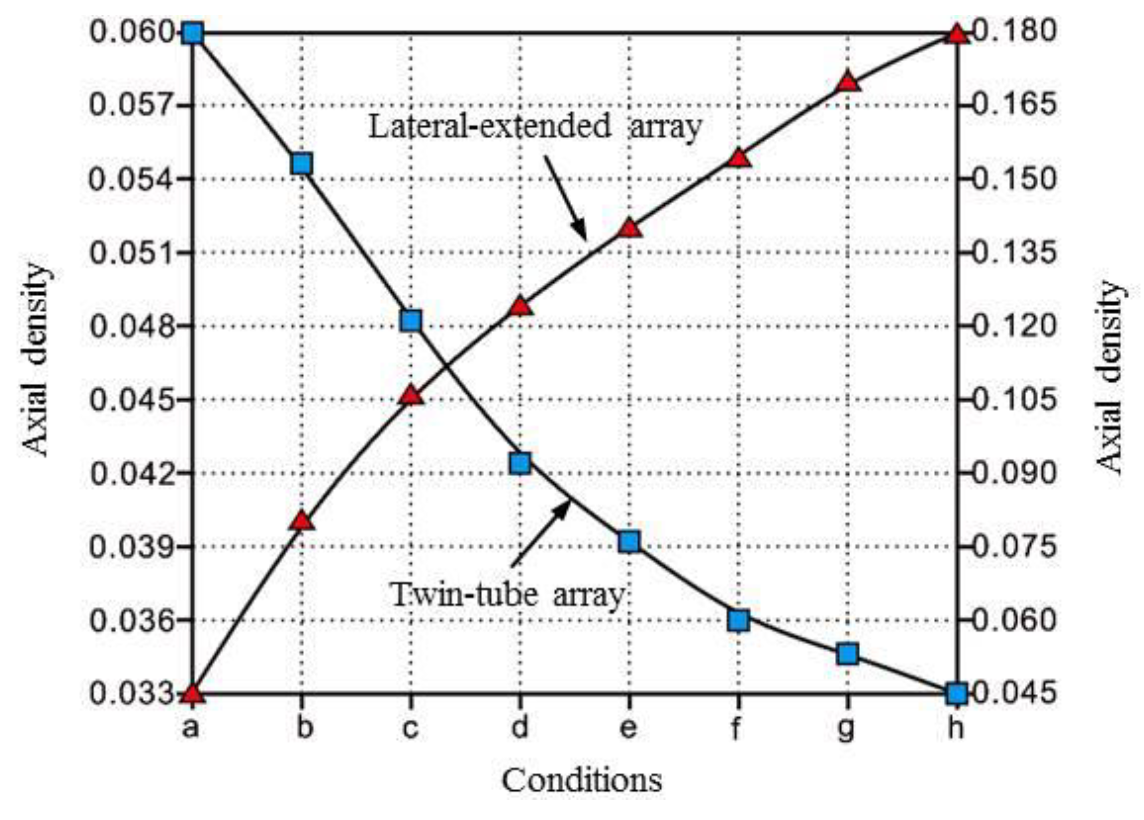
The exploitation of three non-enclosed microseismic arrays in deep-buried tunnels was discussed. The axial-extended array cannot effectively enhance the accuracy of the source location along the axial direction. The lateral-extended and twin-tube arrays efficiently improved the accuracy of the source location of the monitoring range, but the lateral-extended layout was limited by the construction conditions of the tunnels, while the twin-tube array cannot achieve the best source location accuracy in a twin-tube tunnel. In addition, the artificial knock test was used to verify the location accuracy of the three abovementioned non-enclosed arrays, and it was found that a twin-tube array made microseismic events more concentrated. Moreover, the feasibility of using additional microseismic arrays should be explored in conjunction with the proposed method in this paper.

(4)

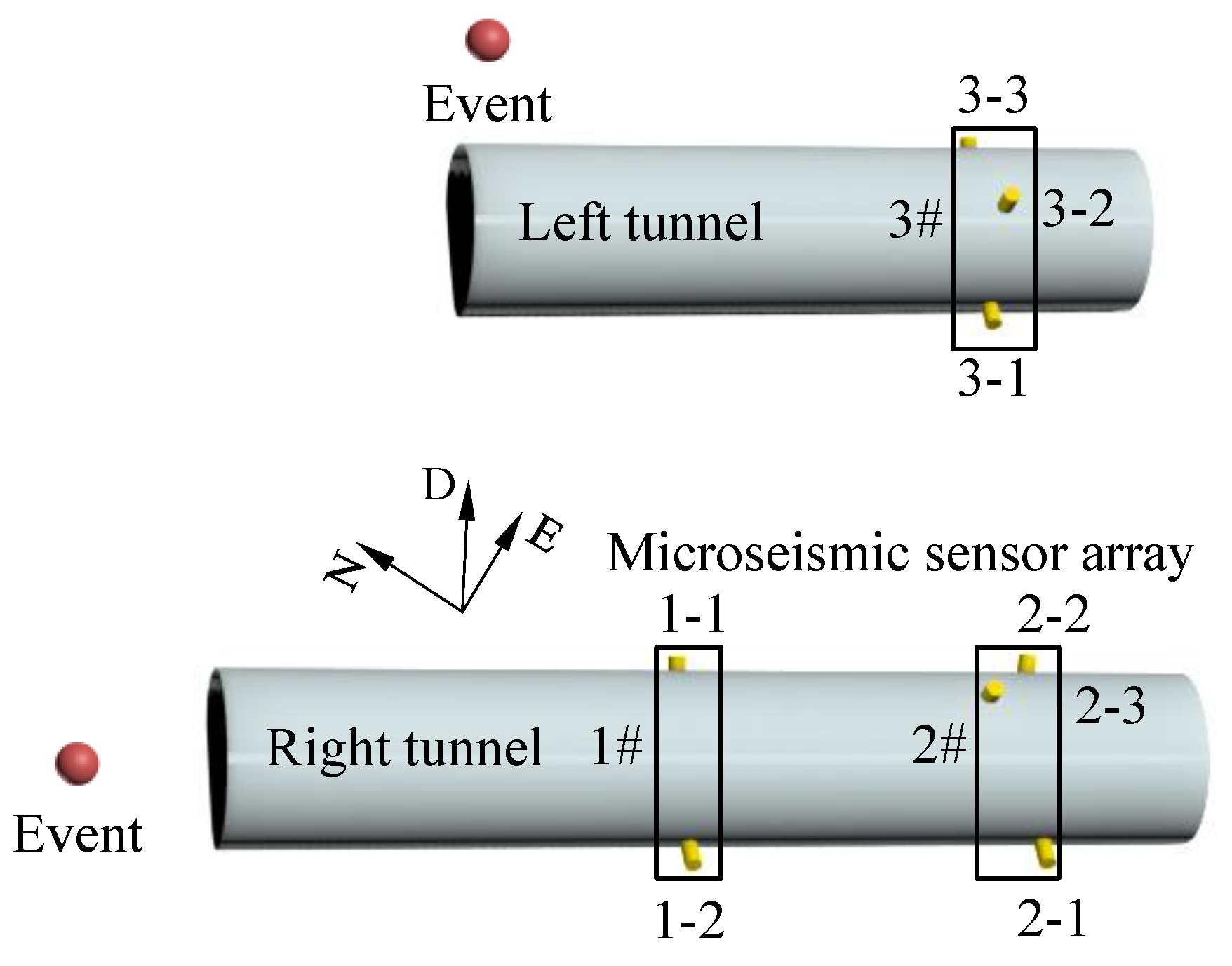
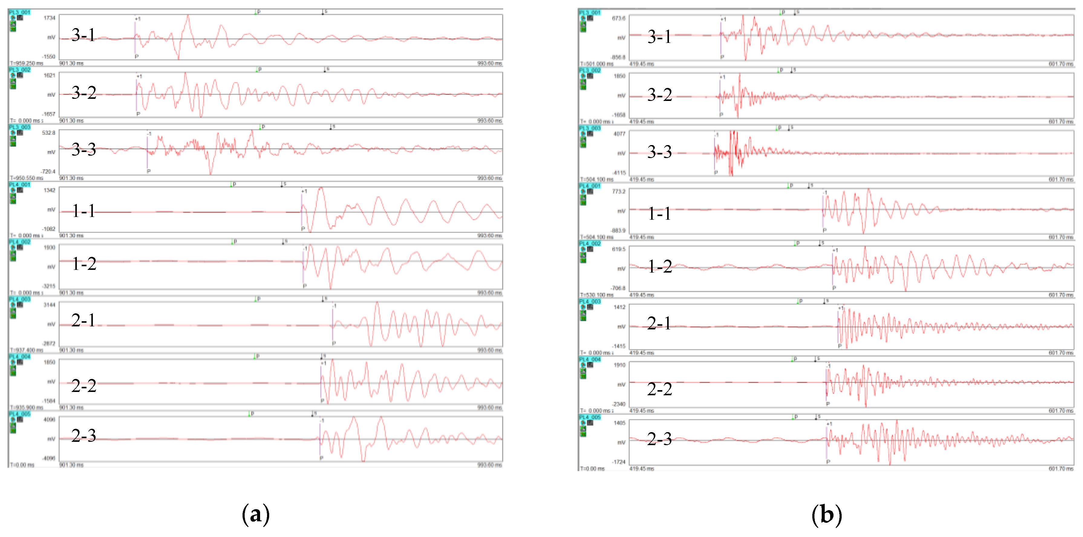
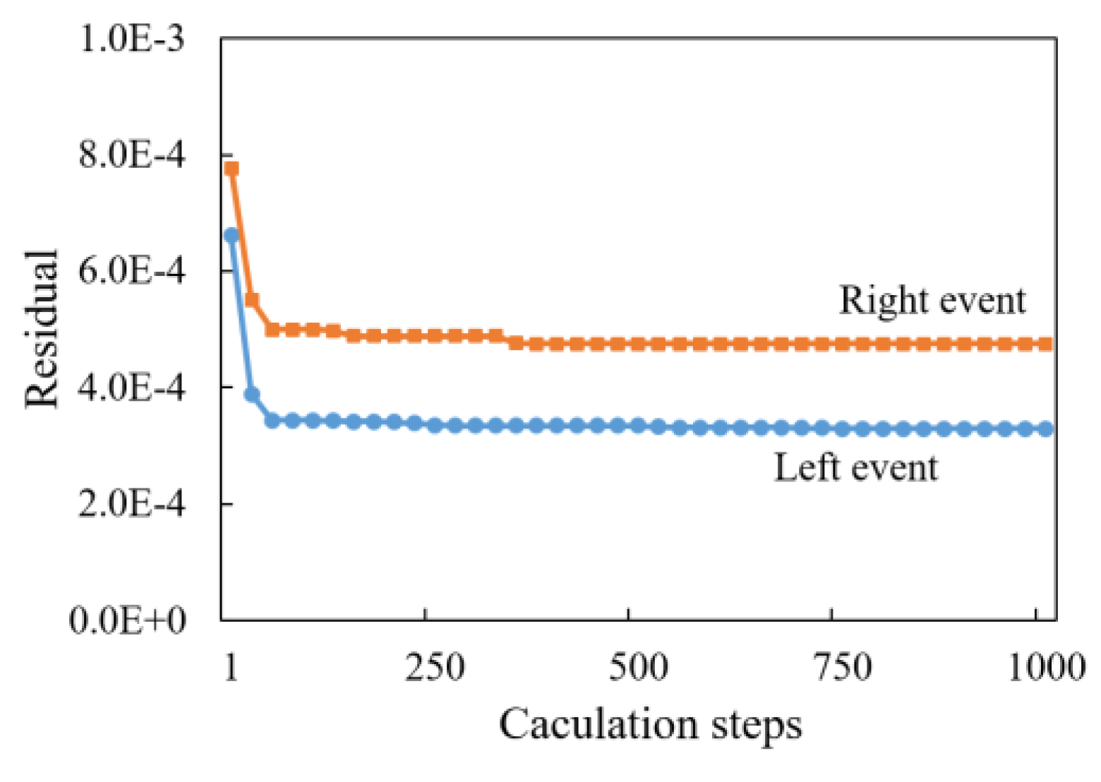
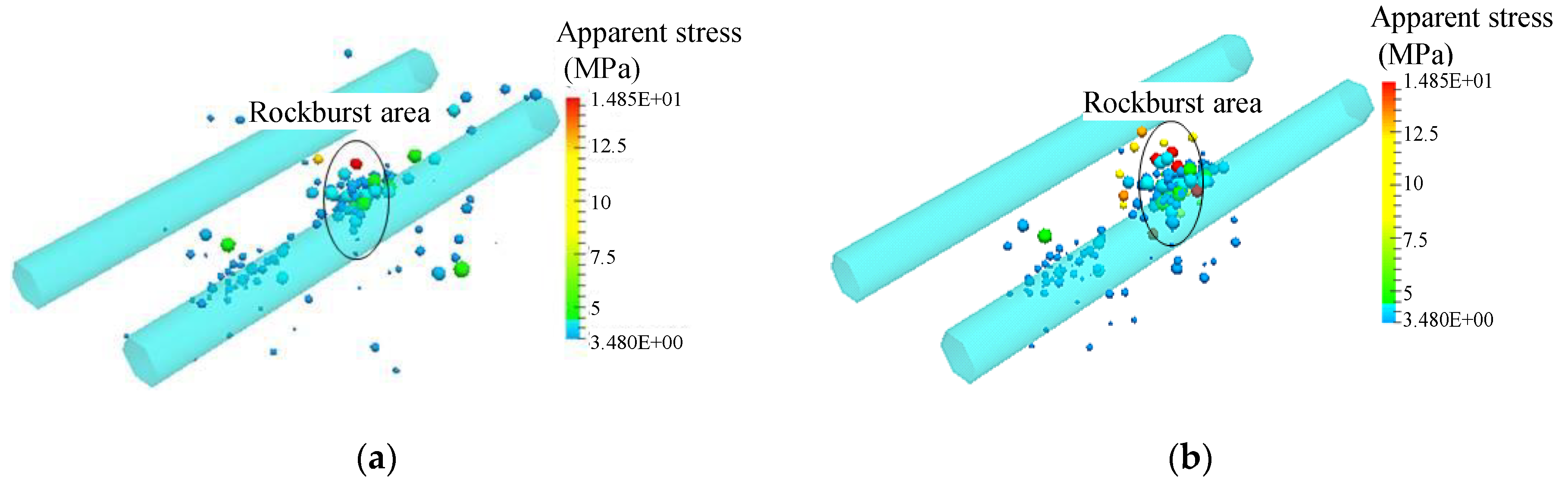
A microseismic monitoring system with a twin-tube array was established and applied to the rockburst area of the Micang Mountain tunnel on the Bashan Expressway. Initially, we were able to identify microseismic events in the left or right tunnels based on the arrival times of the microseismic waves in the twin-tube array. Moreover, based on the PSO, the twin-tube array obtained more accurate locations of the sources than that in the single-tube tunnel, which gathered microseismic events into clusters in the rockburst section and reduced the maximum error by 30–50 m.

The application of the location accuracy of non-enclosed microseismic sensor arrays provide a reference for further studying microseismic monitoring technologies for underground tunnel disasters. Through the analysis of the development rate of microseismic events, the release of energy and the evolution of source parameters in the damaged areas of rock masses, dynamic monitoring and early warning of tunneling rockburst disasters can be realized.

References

1. Hassani, H.; Hlousek, F.; Alexandrakis, C.; Buske, S. Migration-based microseismic event location in the Schlema-Alberoda mining area. Int. J. Rock Mech. Min. Sci. 2018, 110, 161–167. [Google Scholar] [CrossRef]
2. Xu, N.; Tang, C.; Li, L.; Zhou, Z.; Sha, C.; Liang, Z.; Yang, J. Microseismic monitoring and stability analysis of the left bank slope in Jinping first stage hydropower station in southwestern China. Int. J. Rock Mech. Min. 2011, 48, 950–963. [Google Scholar] [CrossRef]
3. Ma, C.; Li, T.; Xing, H.; Zhang, H.; Wang, M.; Liu, T.; Chen, G.; Chen, Z. Brittle rock modeling approach and its validation using excavation-induced micro-seismicity. Rock Mech. Rock Eng. 2016, 49, 3175–3188. [Google Scholar] [CrossRef]
4. Zhao, J.; Feng, X.; Jiang, Q.; Chen, B.; Xiao, Y.; Hu, L.; Feng, G.; Li, P. Analysis of microseismic characteristics and stability of underground caverns in hard rock with high stress using framing excavation method. Rock Soil Mech. 2018, 39, 1020–1027. (In Chinese) [Google Scholar]
5. Xue, Q.; Wang, Y.; Zhai, H.; Chang, X. Automatic Identification of Fractures Using a Density-Based Clustering Algorithm with Time-Spatial Constraints. Energies 2018, 11, 563. [Google Scholar] [CrossRef]
6. Tezuka, K.; Niitsuma, H. Stress estimated using microseismic clusters and its relationship to the fracture system of the Hijiori hot dry rock reservoir. Eng. Geol. 2000, 56, 47–62. [Google Scholar] [CrossRef]
7. Wang, P.; Chang, X.; Zhou, X. Estimation of the Relative Arrival Time of Microseismic Events Based on Phase-Only Correlation. Energies 2018, 11, 2527. [Google Scholar] [CrossRef]
8. Ma, C. Microseismic Monitoring of Brittle Fracturing of Surrounding Rock in Deep-buried Tunnel and Study on Interpretation and Early-warning of Rock Burst. Ph.D. Thesis, Chengdu University of Technology, Chengdu, China, 2017. [Google Scholar]
9. Ma, C.; Jiang, Y.; Li, T.; Chen, G. Microseismic Characterization of Brittle Fracture Mechanism in Highly Stressed Surrounding Rock Mass. In Proceedings of the 25th International Conference and Exhibition—Interpreting the Past, Discovering the Future, Adelaide, Australia, 21–24 August 2016. [Google Scholar]
10. Ma, C.; Li, T.; Zhang, H.; Wang, J. An evaluation and early warning method for rockburst based on EMS microseismic source parameters. Rock Soil Mech. 2018, 39, 765–774. (in Chinese). [Google Scholar]
11. Wang, S.; Li, C.; Yan, W.; Zou, Z.; Chen, W. Multiple indicators prediction method of rock burst based on microseismic monitoring technology. Arab J. Geosci. 2017, 10, 132. [Google Scholar] [CrossRef]
12. Zhang, H.; Chen, L.; Chen, S.; Sun, J.; Yang, J. The Spatiotemporal Distribution Law of Microseismic Events and Rockburst Characteristics of the Deeply Buried Tunnel Group. Energies 2018, 11, 3257. [Google Scholar] [CrossRef]
13. Kijko, A. An algorithm for the optimum distribution of a regional seismic network-I. Pure Appl. Geophys. 1997, 115, 999–1009. [Google Scholar] [CrossRef]
14. Kijko, A. An algorithm for the optimum distribution of a regional seismic network-II: An analysis of the accuracy of location of local earthquakes depending on the number of seismic stations. Pure Appl. Geophys. 1997, 115, 1011–1021. [Google Scholar] [CrossRef]
15. Mendecki, A.J. Seismic Monitoring in Mines; Chapman and Hall Press: London, UK, 1997. [Google Scholar]
16. Ge, M. Analysis of Source Location Algorithms, Part I: Overview and Non-Iterative Methods. J. Acoust. Emiss. 2003, 21, 14–28. [Google Scholar]
17. Ge, M. Analysis of source location algorithms, Part II: Iterative methods. J. Acoust. Emiss. 2003, 21, 29–51. [Google Scholar]
18. Chen, B.; Feng, X.; Zeng, X.; Xiao, Y.; Zhang, Z.; Ming, H.; Feng, G. Real-time micro-seismic monitoring and its characteristic analysis during TBM tunneling in deep-buried tunnel. Chin. J. Rock Mech. Eng. 2011, 30, 275–283. (In Chinese) [Google Scholar]
19. Huang, M. Study on the Mechanism and Micro-seismic Monitoring for Rock Burst in Deep Tunnels. Master’s Thesis, Dalian University of Technology, Dalian, China, 2011. [Google Scholar]
20. Li, N.; Wang, E.; Li, B.; Wang, X.; Chen, D. Research on the influence law and mechanisms pf sensors network layouts for the source location. J. Chin. Uni. Min. Tech. 2017, 46, 229–236. [Google Scholar]
21. Dong, L.; Li, X. Three-dimensional analytical solution of acoustic emission or microseismic source location under cube monitoring network. Trans. Nonferrous Met. Soc. China 2012, 22, 3087–3094. [Google Scholar] [CrossRef]
22. Kijko, A.; Sciocatt, M. Optimal spatial distribution of seismic stations in mines. Int. J. Rock Mech. Min. Geomech. Abstr. 1995, 32, 607–615. [Google Scholar] [CrossRef]
23. Ge, M. Source location error analysis and optimization methods. J. Rock Mech. Rock Eng. 2012, 4, 1–10. [Google Scholar] [CrossRef] [Green Version]
24. Li, N. Research on Mechanisms of Key Factors and Reliability for Microseismic Source Location. Ph.D. Thesis, China Mining University, Xuzhou, China, 2014. [Google Scholar]
25. Li, N.; Wang, E. Mechanism and Application of Key Factors for Micro-epicenter Positioning; China University of Mining and Technology Press: Xuzhou, China, 2015. [Google Scholar]
26. Li, N.; Wang, E.; Ge, M.; Sun, Z. A nonlinear microseismic source location method based on Simplex method and its residual analysis. Arabian J. Geosci. 2014, 7, 4477–4486. [Google Scholar] [CrossRef]
27. Kennedy, J.; Eberhart, R. Particle swarm optimization. In Proceedings of the IEEE International Conference on Neural Networks, Perth, Australia, 27 November–1 December 1995; pp. 1942–1948. [Google Scholar]
28. Shi, Y.; Eberhart, R. A modified particle swarm optimizer. In Proceedings of the IEEE Conference on Evolutionary Computation, Anchorage, AK, USA, 4–9 May 1998; pp. 69–73. [Google Scholar]
29. Rezaee, J.; Jasni, J. Parameter selection in particle swarm optimization: A survey. J. Exp. Theor. Artif. Intell. 2013, 25, 527–542. [Google Scholar] [CrossRef]
Figure 1. Waveforms of microseismic signals. T i and t i in order represent the data of the i-th sensor and the observed arrival time of the i-th sensor.
Energies 12 02006 g001
Figure 2. Microseismic sensor array and residual space: (a) layout of the microseismic array; (b) residual space in the A-H plane, and the location error in the axial direction is the greatest.
Energies 12 02006 g002
Figure 3. Hyperbolic domain of the sensor and array center. The residual variation rate in the axial direction, A n , can be improved by adjusting the sensors T i and T 0 .
Energies 12 02006 g003
Figure 4. Crossed hyperbolic domain. The residual variation rate in the axial and horizontal direction, A n and H n , can be improved by adjustment of the sensors T i , T j , and T 0 .
Energies 12 02006 g004
Figure 5. Lateral-extended array and residual space: (a) lateral-extended array placement; (b) residual space in the A-H plane, and the maximum value of the residual variation rate is 8.18 × 10⁻⁴, and the residual space effect also exits in the axial direction.
Energies 12 02006 g005
Figure 6. Distribution curve of hyperbolic density along the axial direction of the tunnel. The hyperbolic density along the axial direction of the tunnel improves from 0.033 to 0.060 as the buried depth increases from 3 m to 24 m in the lateral-extended array, and which decreases from 0.180 to 0.045 with the sensor array position of the forward tunnel moving to the rear from 0 m to 70 m in the twin-tube array.
Energies 12 02006 g006
Figure 7. Twin-tube array and residual space: (a) twin-tube tunnel array; (b) residual space in the A-H plane, and the maximum value of the residual variation rate is 2.77 × 10⁻³, and the residual space no longer exists in the axial direction.
Energies 12 02006 g007aEnergies 12 02006 g007b
Figure 8. Artificial knock test: (a,b) establishment of microseismic system and installation of sensor arrays; (c) coordinates of knock test point measured by total station; (d) hammer is used to hit the test point to excite artificial waves.
Energies 12 02006 g008
Figure 9. Experimental results obtained from non-enclosed arrays. The size and color of the sphere represent energy (J) and moment magnitude, respectively. (a) Axial-extended array; the sensors located on the left and right walls of each row were 20 m apart from each other in the axial direction; (b) lateral-extended array; the buried depths of the sensors were only extended to 6 m, and the distance between each monitoring section was 30 m; (c) twin-tube array; 9 sensors were arranged in the forward and backward tunnels to monitor the two tunnels well.
Energies 12 02006 g009
Figure 10. Figures (a,b) are the plan and vertical view of arrangement of microseismic monitoring for the twin-tube expressway tunnel: (1) forward tunnel; (2) backward tunnel; (3) sensor array; (4) cable; (5) data acquisition station; (6) data processing station; (7) cross hole; (8) secondary lining.
Energies 12 02006 g010
Figure 11. Twin-tube array for microseismic monitoring of the Micang Mountain tunnel with three monitoring sections. The red sphere represents the microseismic event.
Energies 12 02006 g011
Figure 12. Arrival times of microseismic events as indicated by the array of sensors: (a) arrival time of an event in the right tunnel, the arrival time of Section 1 was earlier than that of Section 2, and Section 3 in the left tunnel had the earliest arrival time due to the complexity of the properties of the surrounding rock and the cavity; (b) arrival time of an event in the left tunnel. The arrival time of Section 3 was the earliest, and the arrival time at the positive side with three sensors (i.e., 1-1, 2-2, and 2-3), was earlier than that at the dorsal side with two sensors (i.e., 1-2 and 2-1).
Energies 12 02006 g012
Figure 13. Search process for each dimension of PSO optimal sample: (a) event in the right tunnel; (b) event in the left tunnel. The horizontal coordinate represents the calculation step, and the vertical coordinate represents the calculation coordinate and velocity, respectively.
Energies 12 02006 g013
Figure 14. Search process for the residual value of the PSO optimal sample. The calculation results of the residual error of the right and left event finally tend to be stable.
Energies 12 02006 g014
Figure 15. Distribution of microseismic events during rockburst in the Micang Mountain tunnel: (a) location based on single-tube array; (b) location based on twin-tube array. Spheres represent a microseismic event and their color represents apparent stress.
Energies 12 02006 g015