Application of Spectral Kurtosis to Characterize Amplitude Variability in Power Systems’ Harmonics

Abstract

The highly-changing concept of Power Quality (PQ) needs to be continuously reformulated due to the new schemas of the power grid or Smart Grid (SG). In general, the spectral content is characterized by their averaged or extreme values. However, new PQ events may consist of large variations in amplitude that occur in a short time or small variations in amplitude that take place continuously. Thus, the former second-order techniques are not suitable to monitor the dynamics of the power spectrum. In this work, a strategy based on Spectral Kurtosis (SK) is introduced to detect frequency components with a constant amplitude trend, which accounts for amplitude values’ dispersion related to the mean value of that spectral component. SK has been proven to measure frequency components that follow a constant amplitude trend. Two practical real-life cases have been considered: electric current time-series from an arc furnace and the power grid voltage supply. Both cases confirm that the more concentrated the amplitude values are around the mean value, the lower the SK values are. All this confirms SK as an effective tool for evaluating frequency components with a constant amplitude trend, being able to provide information beyond maximum variation around the mean value and giving a progressive index of value dispersion around the mean amplitude value, for each frequency component.

1. Introduction

The current electric power system requires extensive control power electronics within all the stages, from the energy generation stage to consumption units (e.g., inverters, rectifiers, DC/DC converters, etc.) [1,2,3,4]. All those power electronics have their own switching frequency, introducing those frequencies in the resultant signal, joined with their harmonics. In addition, non-linear loads, magnetic cores’ saturation, or power unbalance introduce frequencies that are multiples and non-multiples of the fundamental one (harmonics, inter-harmonics, and supra-harmonics), as well. Lower frequencies than the fundamental one (the so-called sub-harmonics) also appear.

Calculation techniques can be classified by the statistical order, based on the order of the moment used. Moments have many formulations due to their being few parameters, but the order is related to the maximum number of times input data are multiplied in the same term by itself (the same or other index). A differentiation is made among first- (no multiplication among them) and second-order methods (two elements are multiplied among them, the most common) and Higher-Order Statistics (HOS), where the order is three or more (three or more elements are multiplied among them).

In order to assess the power system distortion level, the traditional procedures have been designed on three main methodological lines: Discrete Fourier Transform (DFT), Wavelet Transforms (WT) [5,6], and recursive-based methods. The two former ones are purely second-order methods, and the latter incorporate many procedures, such as the Kalman filter [7], neural networks [8], the gravity search algorithm [9], the biogeography hybridized algorithm [10], the hybrid firefly algorithm [11], etc. The convergence of the recursive methods is related to signal conditions, so the accuracy changes. On the other hand, wavelet transform results are related to the mother wavelet used [12]. For all these reasons, DFT is the only technique selected by UNE-EN 61000-4-30 [13] and UNE-EN 61000-4-7 [14] for spectral measurement in Power Quality (PQ) evaluation. DFT still has the second-order characteristics, which makes it vulnerable to noise, and it cannot provide characterization beyond the second order.

In PQ, harmonics are measured as instantaneous and time-averaged values, according to the regulations. This work focuses on the detection of frequency components (sub-harmonics, harmonics, or inter-harmonics) with a constant amplitude trend, which implies a permanent distortion; otherwise, a transitory state may be present during the averaged time or the amplitude values may change. Therefore, DFT will be compared with Spectral Kurtosis (SK), a fourth-order technique (HOS), which shows a very good capacity for different stationary signals [15,16]. It has been previously used in PQ evaluation in [17,18,19] (in addition to other fields, such as insect detection based on vibration [20] or the main application up to now, which is fault detection in rotatory machines [21]), where SK was used for the detection of PQ events, as well as their characterization. In this work, the best configuration for DFT and SK will be studied, for the detection of frequency components with a constant amplitude trend.

The work is structured as follows: In Section 2, SK is studied, then a comparison is made between DFT and SK for detection in Section 3. Then, detection is tested with the current of the arc furnace in Section 4 and with the voltage of the power grid in Section 5. Finally, the conclusions are presented in Section 6.

2. Spectral Kurtosis

While the DFT and the classical power spectral density return amplitude values, without considering any kind of non-stationary information, the SK can target the presence of transients. Indeed, the SK returns the fourth-order statistical moment for each frequency component and, therefore, constitutes a measure of the statistical kurtosis. Thus, unlike the standard deviation, its value is not related to the averaged amplitude, but to the distribution peakedness.

For the SK calculation, the analysis vector must be split into a non-overlapping set of realizations (or segments), and the FFT is applied over them. According to the UNE-EN 61000-4-7, for spectral measurements in PQ, realizations must have a $0.2$-s length (i.e., $10/12$ cycles of $50/60$ Hz). The results of DFT for all realizations are introduced in Equation (1), where the magnitude $X_i\left(m\right)$ estimates the mth frequency component under the ith realization index.

$$SK\left(m\right)=\frac{M}{M-1}\left[\frac{\left(M+1\right){\sum }_{i=1}^M{\left|X_i\left(m\right)\right|}^4}{{\left({\sum }_{i=1}^M{\left|X_i\left(m\right)\right|}^2\right)}^2}-2\right]$$

(1)

The calculation is done for each frequency component, using the estimated amplitude at that frequency for each realization obtained with DFT, as indicated in [15].

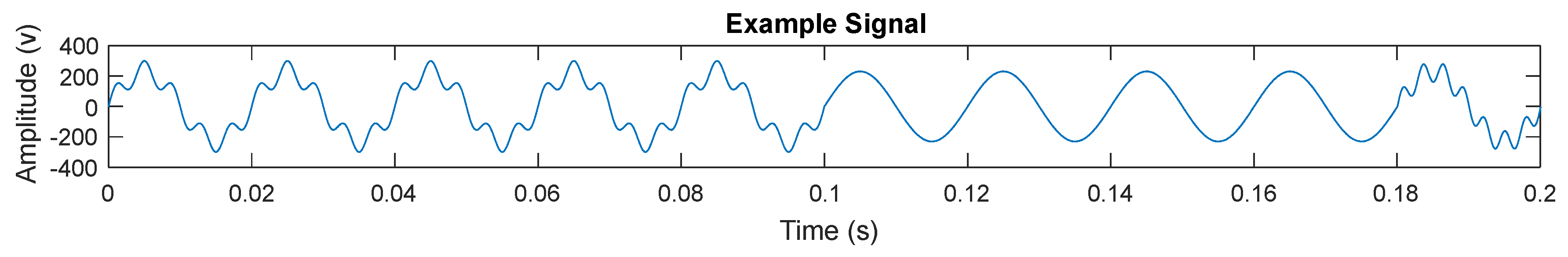
To illustrate the procedure, a preliminary example signal (Figure 1) is first analyzed. It is based on a constant amplitude 50-Hz signal, with 230 V and a 2-s length, and different Signal-to-Noise-Ratios (SNR) of coupled random Gaussian noise are considered (10, 20, 30, 40, 50 dB; 50 in the figure and the others for the analysis). Two harmonics are introduced, without a constant amplitude. The fifth harmonic has 30% of the amplitude, in relation to the fundamental one, during the first half of the signal (1 s), and zero amplitude the rest of the time. The seventh has an amplitude of 30% in relation to the fundamental one during the last cycle of the realization. Figure 1 represents one cycle of each realization analyzed. Each realization has a length of $0.2$ s, and 10 realizations are analyzed, obtaining a 2 s-length signal. Ten amplitude values per frequency are consequently obtained.

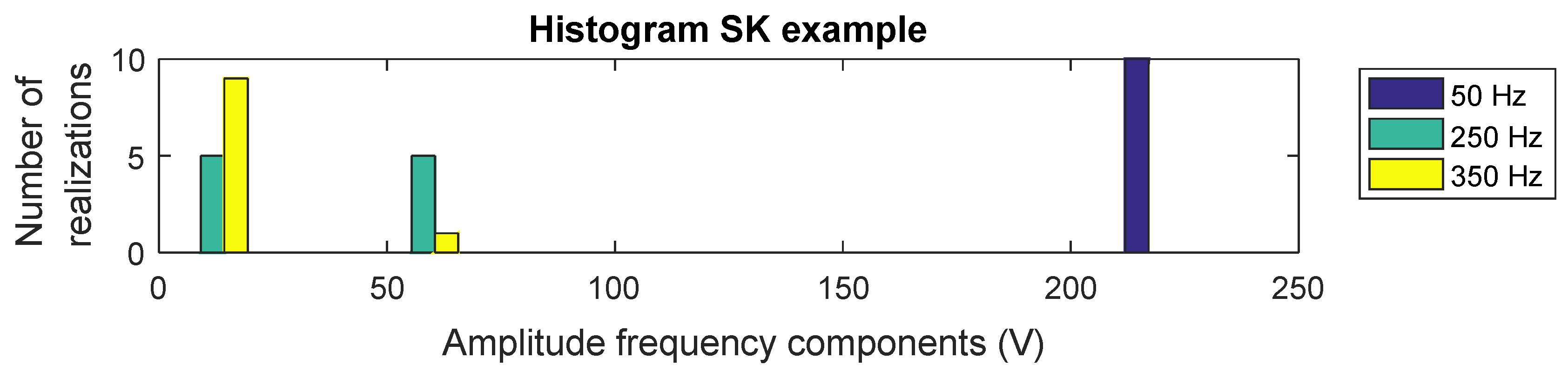
In Figure 2, a histogram of amplitudes is represented for each frequency: 50 Hz (fundamental), 250 Hz (fifth harmonic), and 350 Hz (seventh harmonic).

The histogram shows a constant amplitude for 50 Hz because the ten realizations have the same amplitude. For 250 Hz, half of the points (five) show an amplitude of 70 and the other half zero amplitude. For 350 Hz, only one point shows an amplitude of 70, and the others show zero amplitude. There are three different amplitude value dispersion situations. These amplitude values obtained from DFT are introduced into the SK formula. However, first, these three situations will be theoretically studied over the SK formula. First, if all amplitudes’ values take the same value, the sum result of that value is multiplied by the number of elements summed. With this, the result of Equation (1) is as seen in Equation (2).

$$\begin{array}{c}SK\left(constant\right)=\frac{M}{M-1}\left[\frac{\left(M+1\right)M{\left|X_i\left(m\right)\right|}^4}{{\left(M{\left|X_i\left(m\right)\right|}^2\right)}^2}-2\right]=\frac{M}{M-1}\left[\frac{\left(M+1\right)M{\left|X_i\left(m\right)\right|}^4}{M^2{\left|X_i\left(m\right)\right|}^4}-2\right]=\\ =\frac{M}{M-1}\left[\frac{\left(M+1\right)}{M}-2\right]=\frac{M}{M-1}\left[\frac{\left(M+1-2M\right)}{M}\right]=\frac{M}{M-1}\frac{\left(1-M\right)}{M}=-1\end{array}$$

(2)

Therefore, the ideal returned value for a completely constant amplitude situation is $-1$; noise can affect this, but SK is very noise resistant. The second situation indicated is a signal with the half values with zero amplitude and half the values with an amplitude, which implies a great change (∞ from zero) in half the signal length. In this situation, the sum result is the summed element multiplied by half the number of the added elements. With that, the result of Equation (1) is as seen in Equation (3).

$$\begin{array}{c}SK\left(equal\right)=\frac{M}{M-1}\left[\frac{\left(M+1\right)M/2{\left|X_i\left(m\right)\right|}^4}{{\left(M/2{\left|X_i\left(m\right)\right|}^2\right)}^2}-2\right]=\frac{M}{M-1}\left[\frac{\left(M+1\right)M/2{\left|X_i\left(m\right)\right|}^4}{{(M/2)}^2{\left|X_i\left(m\right)\right|}^4}-2\right]=\\ =\frac{M}{M-1}\left[\frac{M+1}{M/2}-2\right]=\frac{M}{M-1}\left[\frac{M+1-2(M/2)}{M}\right]=\frac{M}{M-1}\frac{1}{M/2}=\frac{2}{M-1}\end{array}$$

(3)

Now, the SK value is a near-to-zero value, nearer as more realizations are used. In the example considered, 10 realization are used, so $2/(10-1)=0.2222$ is obtained. Finally, to simulate impulsive behavior, one point with a non-zero amplitude value and the rest with a zero amplitude value (which implies a punctual ∞ increment) are studied. In this situation, the sum result is a single value of the sum. With that, the result of Equation (1) is as seen in Equation (4).

$$\begin{array}{c}SK\left(max\right)=\frac{M}{M-1}\left[\frac{\left(M+1\right){\left|X_i\left(m\right)\right|}^4}{{\left({\left|X_i\left(m\right)\right|}^2\right)}^2}-2\right]=\frac{M}{M-1}\left[\frac{\left(M+1\right){\left|X_i\left(m\right)\right|}^4}{{\left|X_i\left(m\right)\right|}^4}-2\right]=\\ =\frac{M}{M-1}\left[M+1-2\right]=\frac{M}{M-1}\left[M-1\right]=M\end{array}$$

(4)

Here it can be seen that the SK value for this situation is the number of realizations (actually, it is the maximum SK value that can be returned by SK), in the considered example with 10 realizations. All this was studied in [22]. SK values are shown in

Table 1. SK values for the frequencies in the example signal.

Freq	50 Hz	250 Hz	350 Hz
SNR	SK
10	$-0.9998$	$0.2206$	$9.6754$
20	$-1$	$0.2219$	$9.9774$
30	$-1$	$0.2223$	$9.9945$
40	$-1$	$0.2222$	$9.9994$
50	$-1$	$0.2222$	$9.9998$

.

Noise contamination affects the theoretical values calculated for non-noise-contaminated situations. However, for the five digits represented, for SNR of 20 dB or higher, the constant amplitude situation (50 Hz) is marked with $-1$; only an SNR of 10 dB affects the constant amplitude value.

In relation to the half values affected by the huge amplitude change (250 Hz), with less noise contamination (higher SNR), a value nearer to $0.2222$ (the value calculated for a non-noise situation) is obtained. However, even for the 10-dB SNR situation, $0.2206$ is obtained, which implies an error of less than 1%, and the values are the same as the ideal one for an SNR over 40 dB.

For impulsive behavior (only one point is affected by a huge amplitude increase) (350 Hz), as in the 250-Hz case, as less noise is applied, a value nearer to 10 is obtained. However, with an SNR of 20 dB, an error lower than $0.5$% is obtained, and for an SNR of 50 dB, the error is lower than 20 ppm.

With all this, with an SNR over 20 dB, SK can detect with an acceptable error these three situations, and almost no error for an SNR over 50 dB. Specifically, the constant amplitude is the focus of this work. Additionally, SK has perfectly differentiated two spectral components with the same amplitude change (250 Hz and 350 Hz), but with different time behaviors, an impossible task for a second-order method.

This work is centered on the capacities of the SK for the detection of frequencies with a constant amplitude trend ($-1$ value). This feature is tested by generating variations around a constant level (unitary amplitude). Four signal lengths have been considered: 10, 20, 50, and 200 s (50, 100, 250, and 1000 realizations). Amplitude changes from 10–30% are applied over a length up to 20% of their total lengths. SK has been proven as a noise-resistant technique in the first case. However, in practice, the voltage signal obtained from a power system has an SNR ranging from 50–70 dB [23]. For that, hereinafter, an SNR of 50 dB will be used, due to it having highest contamination in this range. The results of the case are shown in Figure 3.

The horizontal axis shows the relative length of the changed amplitude segment in relation to the whole signal length. The vertical axis shows SK. In this graph, five groups of lines are observed, each one related to a different amplitude change, indicated in the graph on the right. All lines related to the same amplitude change looks like a single line, although they correspond to different signal lengths. This fact illustrates that SK is sensitive to the relative disturbance length in relation to the total signal length, and not the disturbance length. In addition, more amplitude change involves higher SK values. Fifteen percent is needed to get SK over $-0.99$ with a relative length of $12\%$. As higher amplitude change is observed, a smaller defective length would be needed to reach this level. For instance, only a relative length of 6% with an amplitude change of 20% is needed, or a relative length less than 4% with an amplitude change of 25%, or a relative length of 2% with an amplitude change of 30%.

3. SK vs. DFT in the Harmonic Evaluation

In this section, a synthetic signal, based on the one used in [24,25], is studied. This signal represents a typical industry waveform, which comprises the effects of power electronic devices, Variable Frequency Drives (VFDs), and arc furnaces. The signal under test has a 10-s length, with a constant amplitude, up to the ninth harmonic. In addition, temporal harmonic distortion has been introduced in harmonic of orders of 11, 13, and 15. The signal harmonic composition is detailed in

Table 2. Harmonic composition of the signal.

Harm Order	Amp (V)	Phase (${}^{\circ }$)	Evolution	Start (s)	End (s)
1st	1.5	80	Constant	0	10
3rd	0.5	60	Constant	0	10
5th	0.2	45	Constant	0	10
7th	0.15	36	Constant	0	10
9th	0.1	30	Constant	0	10
11th	$0.3$	0	$\Delta 25\%$	$0.9$	$1.1$
13th	$0.3$	0	$\Delta 25\%$	1	2
15th	$0.3$	0	$\Delta 25\%$	$0.9$	$1.2$

. For signal generation, a sampling frequency of 2560 Hz is used, and Gaussian noise is coupled with a 50-dB SNR.

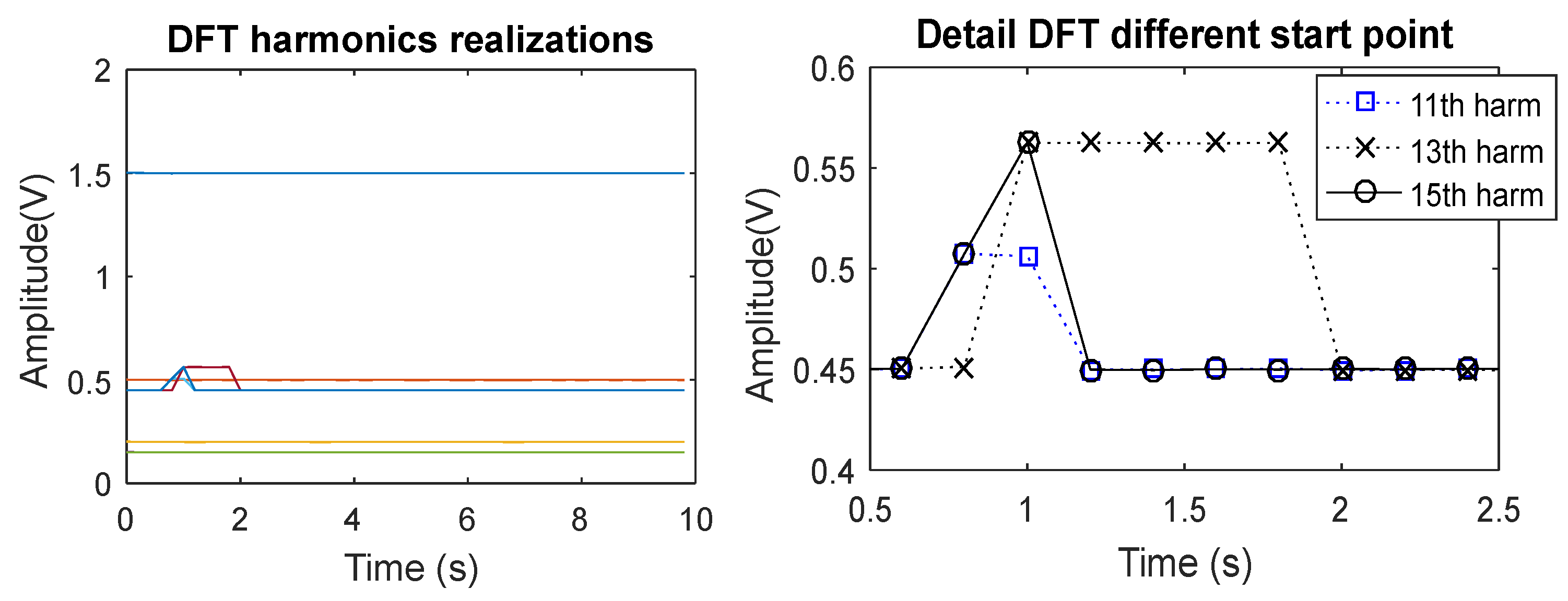
A time domain signal is obtained, composed of multiple frequencies. SK is based on DFT, so first, DFT must be applied. As indicated before, the first step consists of the signal segmentation into $0.2$ s-length realizations (50 realizations are obtained), according to the PQ spectral analysis in UNE-EN 61000-4-30 [13] and UNE-EN 61000-4-7 [14]. The amplitudes returned by DFT are shown in Figure 4. In the left graph, all frequencies involved in this study are shown, and in the right graph, a zoom over the changing amplitude components is applied.

Different levels are observed in the left parts of the graphic representation. All are almost constant, except three of them, which represent the components with frequencies of variable amplitudes. In the graph on the right, paying attention to the 11th harmonic, two points fall outside the normal value. However, the length of this disturbance is the same as the realization length (0.2 s). This is due to the fact that the change of the level starts in one realization and ends in another, so it is shown as two small changes of the level. The 13th and 15th harmonics have a longer changed amplitude length than a realization’s length, so the maximum amplitude change can be read properly. In the 15th harmonic, first, half the realization has an amplitude change, and then, the complete realization has the proper amplitude change. In the 13th harmonic, five realizations with the proper amplitude change are given.

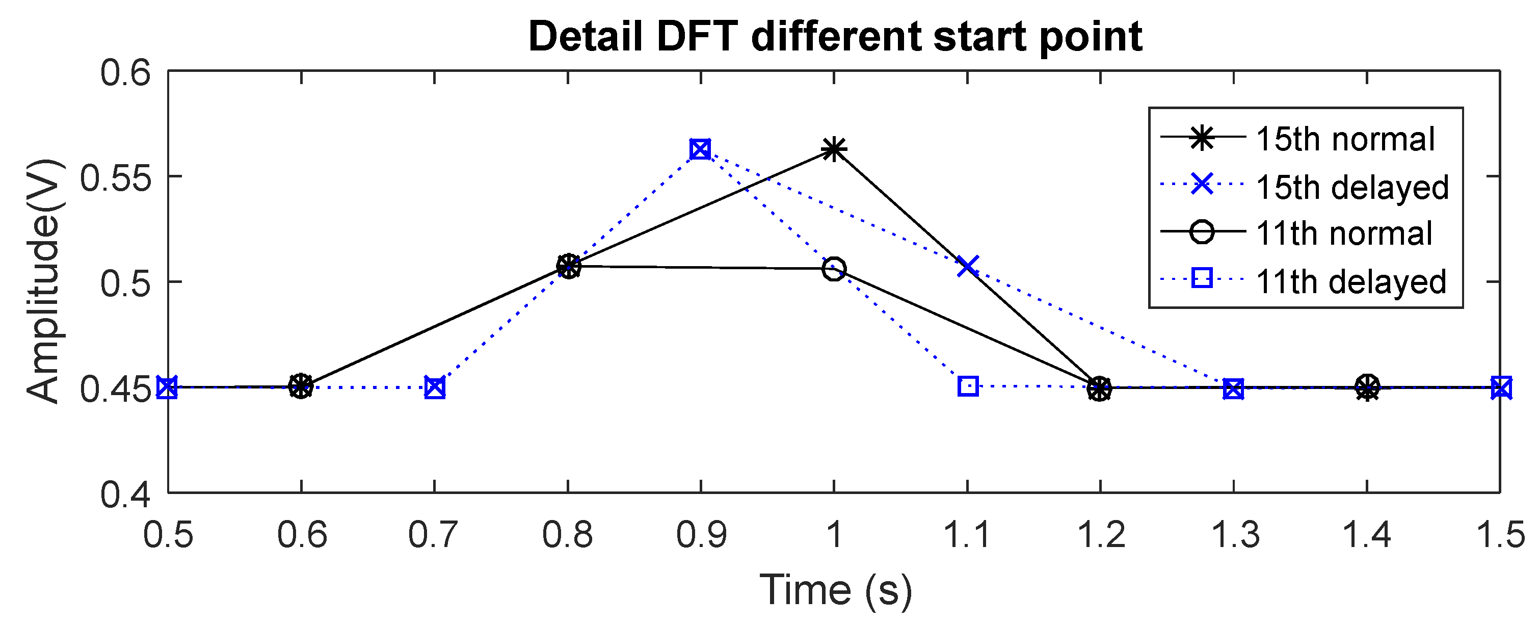
Even having the segment with the amplitude changed, the same length as a realization, the 11th harmonic has been observed as two realizations with the amplitude changed, with a lower amplitude change. This proves that DFT is sensitive to the disturbance starting point, due to the data segmentation performed. However, if we want to perform a detection of the amplitude evolution, this segmentation is needed. Moreover, as said before, this segmentation follows the regulations and standard requirements. In order to maximize the detection capacities, another DFT is calculated, but the starting point is delayed half a realization length. The 11th and 15th harmonics are analyzed again, and the results are shown for both DFTs (normal and delayed) in Figure 5.

The 15th harmonic shows a similar response in the normal and delayed DFT. The only difference that can be observed is that in the normal DFT, the first realization is detected with half the amplitude change and the second one with the maximum amplitude, and the opposite occurs in the delayed DFT. Amplitude change starts in $0.9$ s with a $0.3$-s length. A $0.2$-s length per realization is taken, starting at zero for the normal DFT and starting the delayed one in the second $0.1$ (half the realization length). The starting points are in the middle of a realization for the normal DFT, but at the beginning of a realization for the delayed one.

However, the 11th harmonic shows a different response for the normal and delayed DFT. In normal DFT, it shows the same response previously seen, and in the delayed one the complete amplitude change in one realization can be seen, so delayed DFT reads the full amplitude change in only one realization. The amplitude change starting point links with the realization starting point of delayed DFT and with half the realization length of normal DFT.

With the double DFT, more information is obtained; even more in amplitude change segments with a small length, which can be split into two realizations. This creates a higher amplitude change read in one of the DFTs, due to the disturbance inside a realization and not being split. Therefore, for an amplitude stability analysis, it is recommendable to use the double DFT. However, up to this point, graphs against time have been obtained. In order to show a single value per frequency component, SK is applied. If we want to compare SK and DFT, single values for DFTs need to be obtained per frequency component. These values are the averaged amplitude value, maximum amplitude change, and maximum amplitude change relative to the averaged amplitude value, and they are shown in

Table 3. Single value analysis for different harmonic orders, in DFT Normal (N) and Delayed (D).

Order	3rd		11th		13th		15th
DFT	N	D	N	D	N	D	N	D
Avg	0.50	0.50	0.30	0.30	0.31	0.31	0.30	0.30
Max − Min	0.00	0.00	0.04	0.08	0.08	0.08	0.08	0.08
(Max − Min)/Avg	0.01	0.00	0.13	0.25	0.25	0.25	0.25	0.25
SK	−1.000	−1.000	−0.997	−0.994	−0.973	−0.976	−0.992	−0.992

.

With the averaged amplitude value, the normal amplitude is seen, and it almost does not change, even in the longest amplitude change situations. The maximum amplitude change value is an absolute parameter, and the averaged amplitude value is needed in order to understand the change in relation to the normal situation (relative change). Relative amplitude change in the constant amplitude situation (third harmonic) shows a value of $0.01$, due to noise. For amplitude changing components, a value of $0.25$ is obtained for the 13th and 15th harmonics and delayed DFT of the 11th harmonic (the normal one shows a smaller relative change). It is $25\%$ of the relative change introduced.

All those indicators can detect amplitude change with a single DFT realization out of the indicated conditions, but cannot differentiate among one or more realizations. In this work, we want to study the constant amplitude trend, and with that aim, we need to know if the amplitude change occurs once or if it appears continuously over time. SK values show a value of almost $-1$ for the constant amplitude component, a value near $-0.99$ for a single realization being affected ($0.2$ s of 10 s implies 2%), and $-0.97$ for the amplitude change with a higher length (1 s of 10 s implies 10%). As seen in the previous section, SK can differentiate among short or long length amplitude changes, taking into consideration the amplitude change value as well.

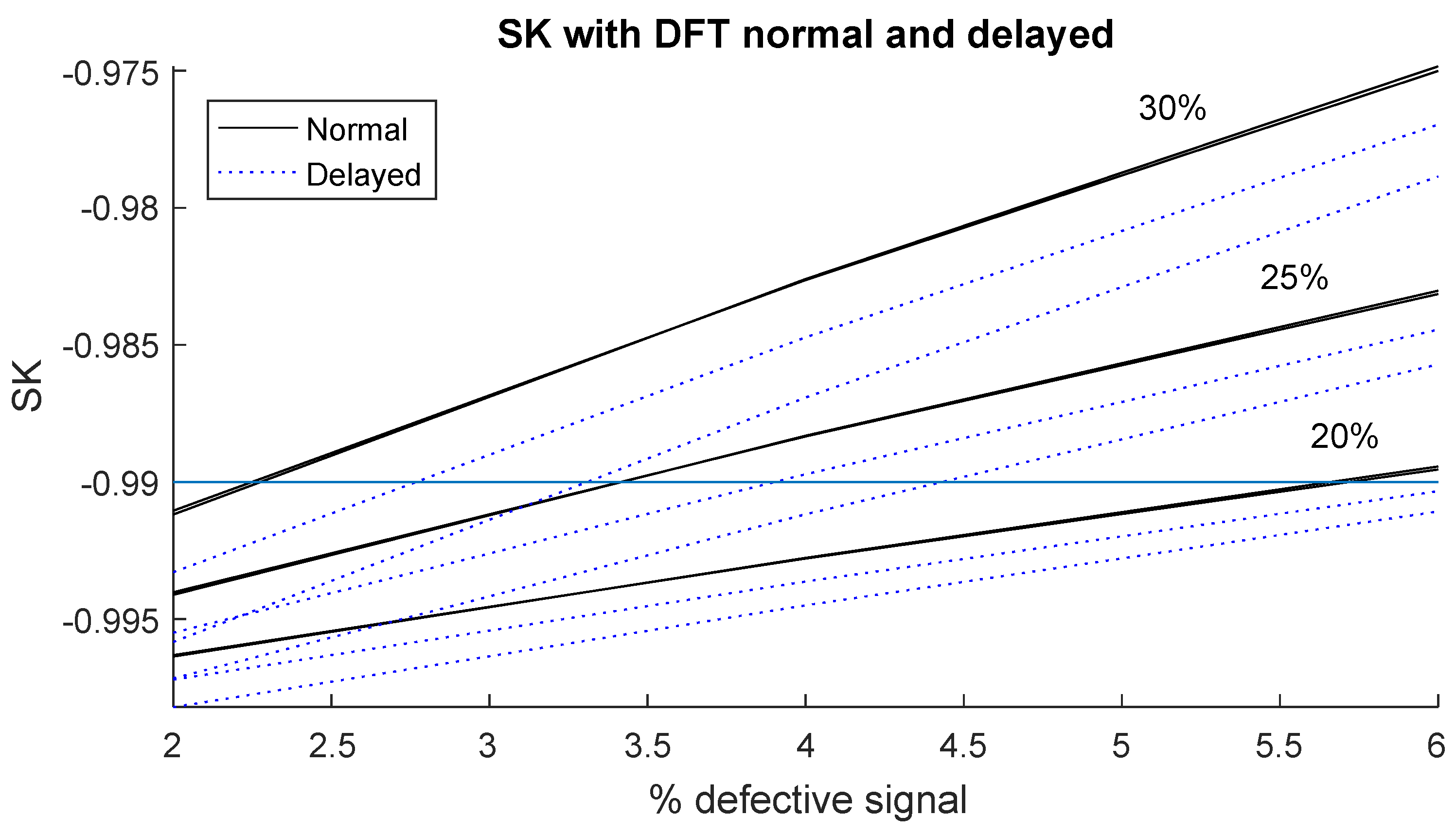
In the 11th harmonic, the amplitude change starting point affects the SK value, so an SK analysis for different starting points must be done. As shown in Figure 3, different relative lengths for the amplitude change segment are considered. Now, two signal lengths are considered, 10 and 20 s. The amplitude change starting point is the starting point of the second realization of normal DFT. Therefore, normal SK sees the amplitude change in the complete realization, and delayed SK splits it. The results of this analysis are shown in Figure 6.

In this figure, it can be observed that delayed SK, the one that splits the amplitude change segment into more realizations, returns lower SK values. Therefore, normal SK returns higher SK values in this situation. If the disturbance starting point changes, delayed SK can show higher values than normal SK. This shows that double SK ensures that the optimum SK value is obtained, associated with the worst situation. The solid line is associated with normal SK, and for both signal lengths, this line is overlapped. However, delayed SK, represented as a dotted line, takes a different position with each signal length. A great difference between the dotted line and solid line can even be seen, the absolute difference being lower than $0.05$. Although the same relative length is used, as a higher total length is considered, less difference is observed. Realization length is constant, and the SK response difference is due to measuring one realization with the full amplitude change or two realizations with half the amplitude change. As more realizations are affected by the amplitude change, this difference has a lower impact.

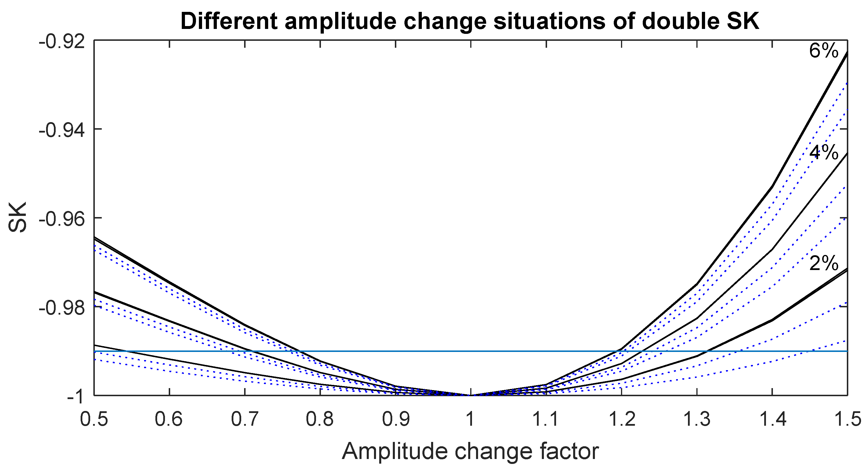
Up to this point, only amplitude increases have been studied. However, if we want to study amplitude stability, increases or reductions can occurs in the amplitude value. Now, an amplitude increase and a reduction of up to 50% have been applied (now, increase or reduction is expressed as “amplitude change factor”, which is the final amplitude/initial amplitude, reduction values below one being being increased values over one), over three different relative lengths (2%, 4%, and 6%) and using two different total lengths (10 and 20 s). The amplitude change starting point, as in the previous simulation, is the second realization of the normal SK. Normal and delayed SK values for this case are shown in Figure 7. An SNR of 50 dB has been considered.

The SK value can be observed for amplitude reduction or increase. Smaller SK values are obtained when the amplitude reduces. As SK is the fourth-order moment, a value increase has more effect, due to it being magnified by the fourth power. As in the previous case, normal SK shows the same values for total length, and delayed SK shows slightly lower values. As more relative length is affected, higher SK values are given. In

Table 4. Amplitude change to reach a −0.99 SK value for different defective lengths.

Relative Length	Amplitude Up	Increment	Amplitude Down	Decrement
2%	1.31	0.31	0.54	0.46
4%	1.22	0.22	0.71	0.29
6%	1.19	0.19	0.77	0.23

, the amplitude change needed for reach $-0.99$ SK values is shown, for the maximum value obtained from the double SK analysis.

As the relative length is affected by amplitude change increases, a smaller amplitude change is needed in order to obtain an SK value over $-0.99$. In this situation, SK under $-0.99$ is the condition to set a frequency component as a constant amplitude trend. As explained up to this point, SK will analyze amplitude changes, not only punctual, but along all of the signal, taking into consideration the duration of each amplitude change.

4. Arc Furnace Current Signal

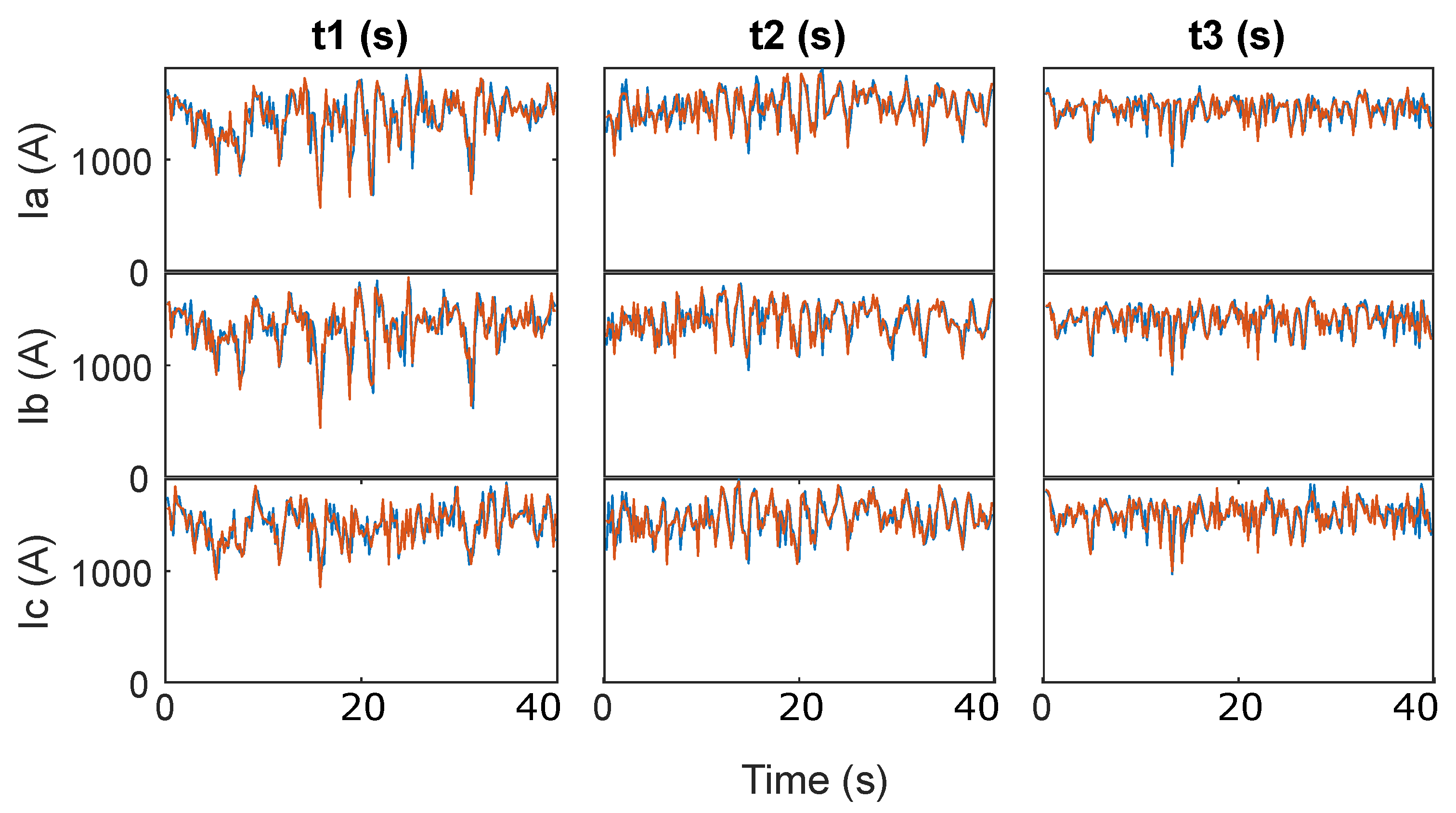
As a real-life application, the electric current waveform from an arc furnace during the melting process is studied, for the three phases, in three time periods. During the melting process, an arc furnace requires a high current level, while it takes a similar level of power during this process. However, the current level is not properly constant, and that situation is a perfect example for the aim of this work. In this situation, low fluctuations are present, and the signal is detected as a constant amplitude trend. In Figure 8, the amplitude values for the current signal can be seen, for the fundamental frequency (50 Hz) measured with DFT. Each segment has a length of 40 s, so with a segmentation of $0.2$ s, 200 realizations result per segment.

In this graph, oscillations in the fundamental component are observed. These oscillations are higher in the first time period, lower in the second one, and much lower in the third one. Moreover, Phases A and B show higher oscillations than Phase C in the first time period. As previously seen, these oscillations will be studied using normal and delayed SK. All SK values for fundamental frequency components are shown in

Table 5. SK values for 50-Hz frequency components in the arc furnace current signal.

	$\mathit{t}1$		$\mathit{t}2$		$\mathit{t}3$
SK	N	D	N	D	N	D
Ia	−0.916	−0.920	−0.963	−0.963	−0.982	−0.982
Ib	−0.923	−0.924	−0.960	−0.958	−0.976	−0.975
Ic	−0.948	−0.948	−0.960	−0.961	−0.976	−0.974

.

As explained before, an SK value of $-1$ is related to a constant amplitude trend, and higher SK values are obtained (more positive or less negative) as higher amplitude variations are observed. In Figure 8, higher amplitude variations are observed in Time Period 1, and due to those oscillations, values in the range of $[-0.948,-0.916]$ are observed, for all phases.

In the second period, a few level variations are observed, lower than in the first one. The SK values obtained are lower also in comparison to the ones obtained in the first period, all of them being in the range of $[-0.963,-0.958]$.

In the third time period, lower variations are observed than in the second one. The SK values obtained are again lower in comparison to those obtained in the second period, all of them being in the range of $[-0.982,-0.974]$.

In addition, if Time Period 1 is observed, as indicated before, lower amplitude variations are observed in Phase C than in Phases A and B. SK values for Phase C are $-0.948,-0.948$ (normal and delayed), and for Phases A and B, SK values are in the range $[-0.916,-0.924]$.

In this case, it is confirmed that as lower amplitude oscillations are observed in the frequency component studied, a lower SK value is obtained. In fact, all SK values are under $-0.9$, due to all amplitude values being near the averaged value. However, none of them obtain an SK value of $-0.99$ or lower, so no constant amplitude trend can be confirmed, even with the amplitude evolution observed in the third period, in Phase A, where amplitude values are really concentrated around the averaged value.

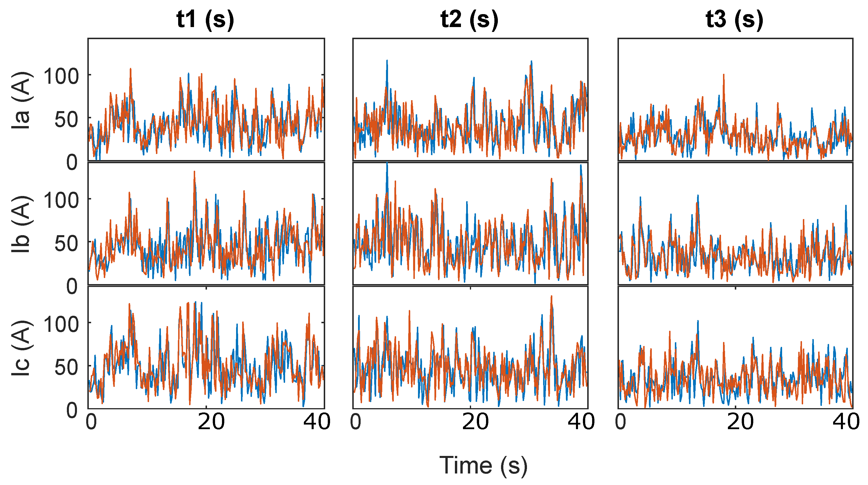
The SK value of zero is associated with noise (random oscillations due to noise). The third harmonic, which only reaches a maximum amplitude around 120 (when the fundamental frequency reaches an amplitude of 1600), implying $7\%$, is studied. It shows random oscillations. Amplitude variations for normal and delayed DFTs for the third harmonic are shown in Figure 9.

In Figure 9, these random amplitude oscillations can be observed, taking values from 0–120. Normal and delayed SK values are shown in

Table 6. SK values for 150-Hz frequency components in the arc furnace current signal.

	$\mathit{t}1$		$\mathit{t}2$		$\mathit{t}3$
SK	N	D	N	D	N	D
Ia	−0.194	−0.105	0.141	0.004	−0.004	0.234
Ib	0.025	0.025	0.074	0.060	0.263	0.082
Ic	0.014	0.015	−0.071	−0.107	0.044	−0.070

.

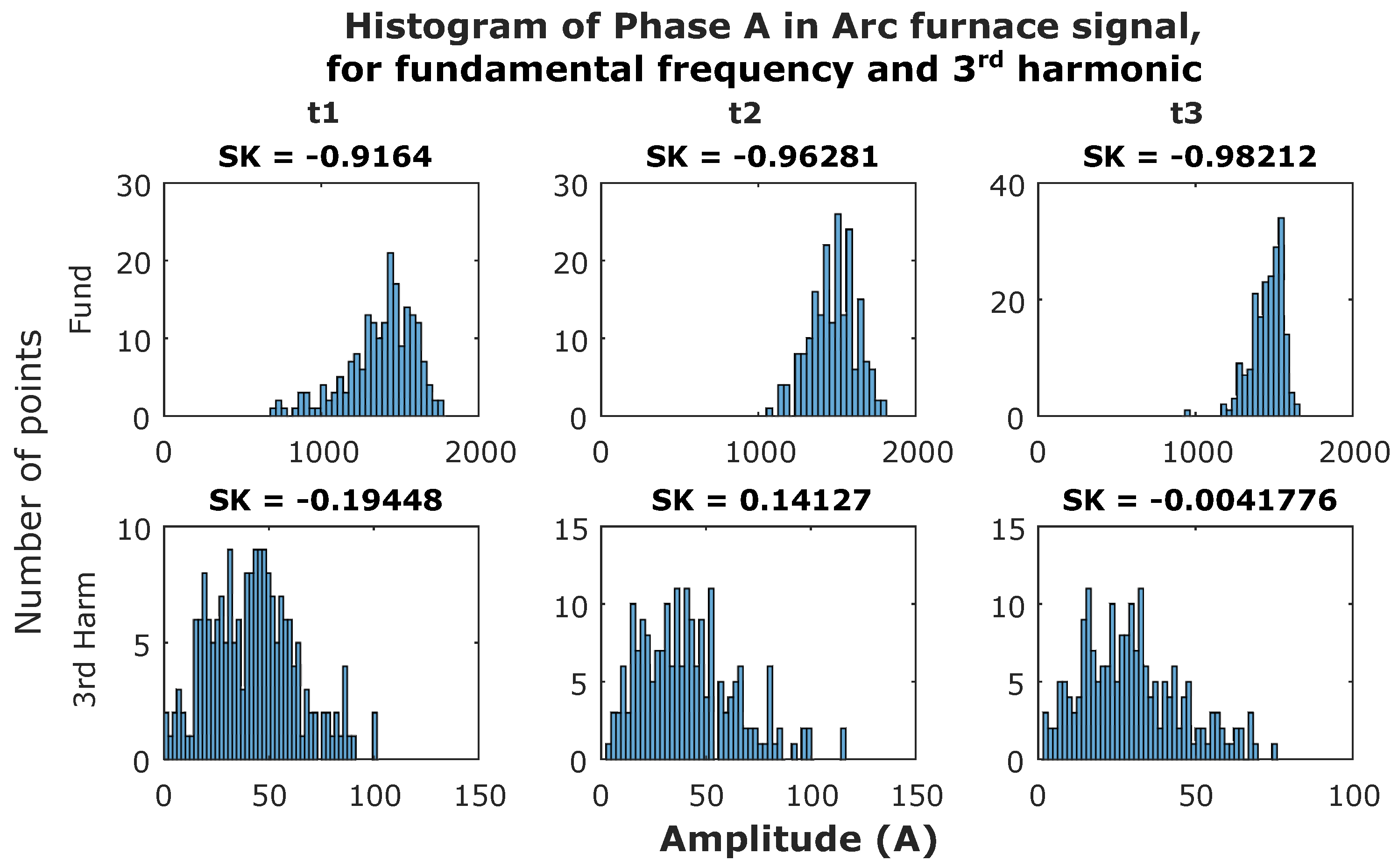
As explained before, random amplitude values are related to a zero SK value, as seen in this table. For all the time periods in all three phases, the SK values obtained are very near to zero. Then, in order to compare amplitude values’ dispersion, histograms for the amplitude values will be represented. A separate histogram is represented for each of the data used. As an example, Phase A is taken for all three time periods in both situations, fundamental frequency, and the third harmonic, resulting in six histograms. Over each histogram, the SK value obtained for that signal is indicated. For histograms, normal DFT is used and normal SK is indicated. Histograms are shown in Figure 10.

Now, in the fundamental frequency, it is easy to see how the values’ concentration around the mean value is related to the SK values, returning lower values as concentration increases. In the third harmonic, it can be observed that amplitude values are not concentrated; they are distributed in a wide range, following a random distribution, associated with a kurtosis of zero (a near to zero value).

5. Power Signal

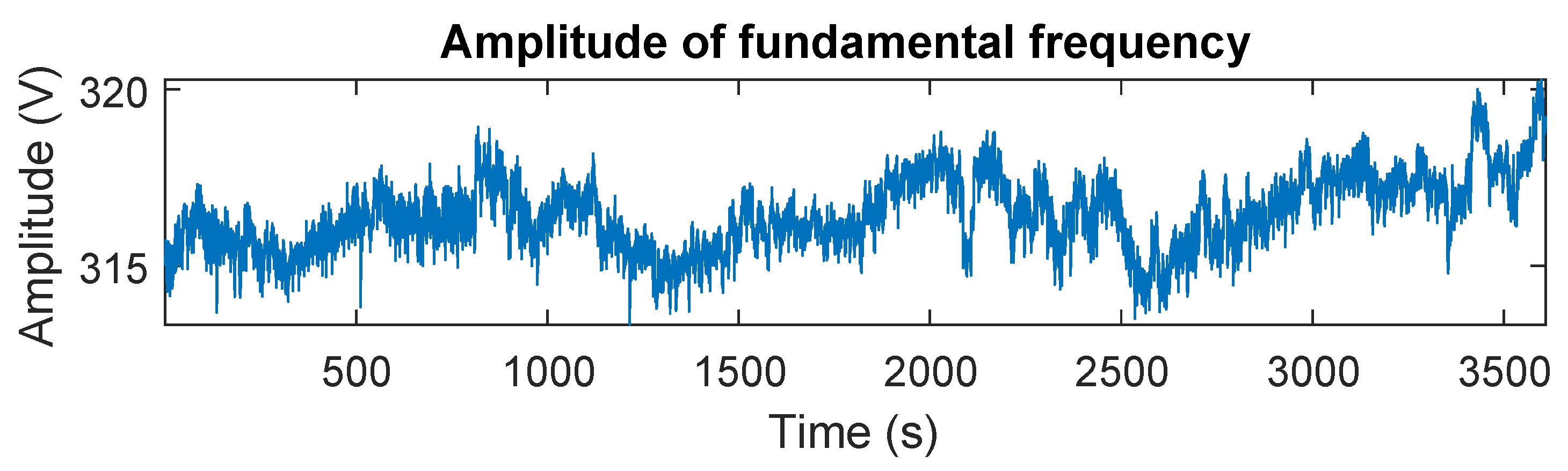
An hour of the voltage waveform from the power grid in the research group laboratory facilities is analyzed. As explained before, a segmentation with $0.2$ s, non-overlapped, has been done, and DFT has been calculated (which resulted in 18,000 realizations). The SK has been calculated over the results of that calculation. First, fundamental amplitude is shown for all segments in Figure 11, as the results of normal DFT.

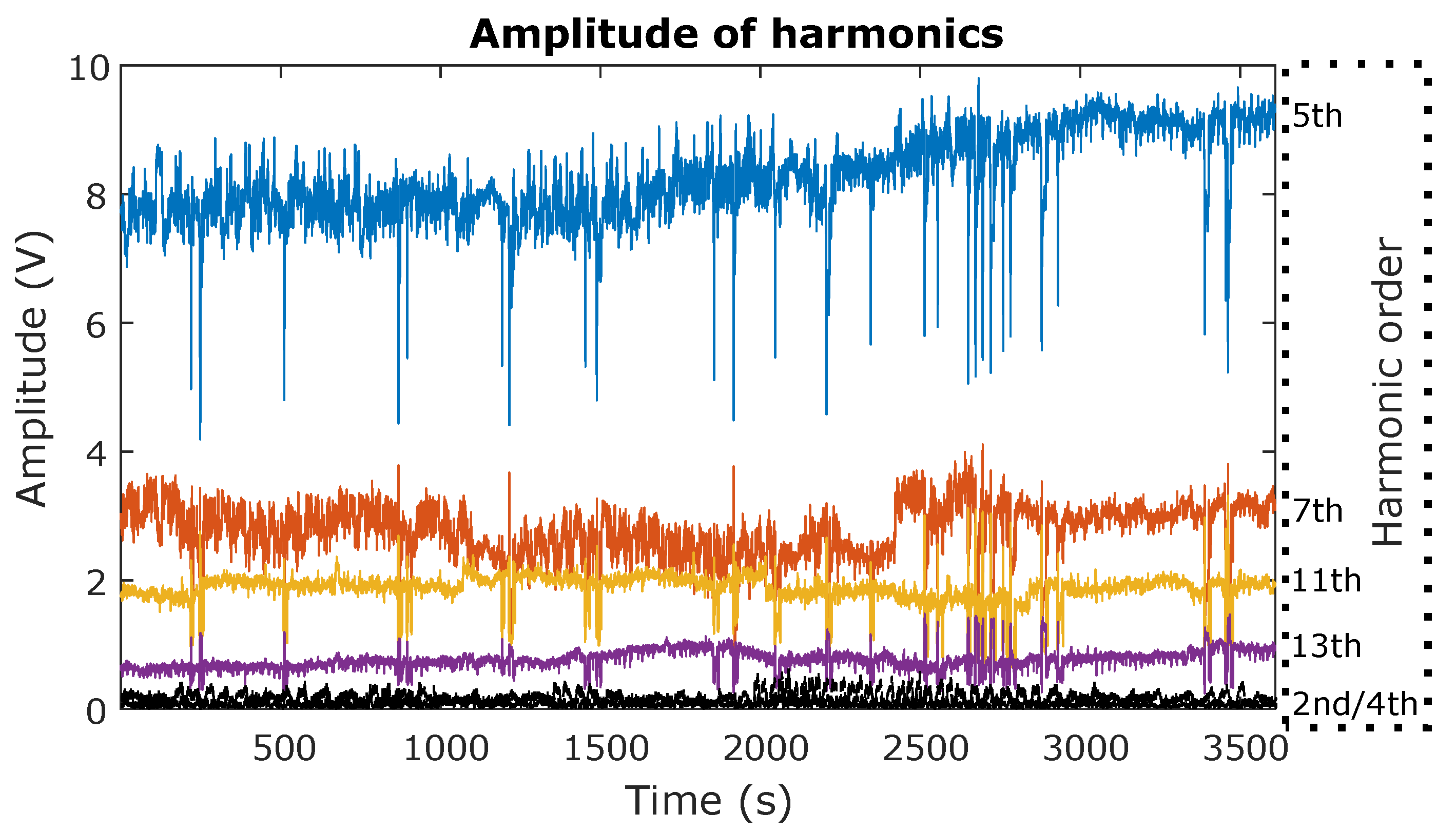
Only small amplitude changes are observed in the fundamental frequency amplitude, taking amplitude values from 314 V–320 V, approximately 2% of variation. The nominal voltage level in Spain, by regulation, is 325 V in amplitude, with an allowed variation margin of $\pm 10$%. The values given are in the allowed range. The amplitude of a few harmonics are studied, due to their amplitude difference. They are plotted in Figure 12, a different figure than was used, due to the amplitude difference from the fundamental one.

The fifth harmonic is the one with a higher amplitude, and even it has an amplitude lower than 3% in relation to the fundamental amplitude. Even with these amplitude differences, SK evaluates amplitude changes in each frequency separately. The second and fourth harmonics have amplitude values centered on zero, with random oscillations. All other harmonics show a evolution around an average value, different for each frequency. They do not show a constant amplitude evolution; each one shows a different evolution, with low amplitude variation.

In

Table 7. SK and DFT values for the studied frequencies in one hour of a power signal.

Harmonic	SK		DFT
Order	N	D	Avg	Max	Min	Inc(%)
1.000	−1.000	−1.000	316.475	320.000	313.000	2
2.000	−0.080	−0.078	0.193	0.698	0.001	361
4.000	0.064	0.066	0.088	0.384	0.001	436
5.000	−0.975	−0.975	8.250	9.581	6.855	33
7.000	−0.919	−0.919	2.755	3.676	1.969	62
11.000	−0.938	−0.938	1.847	2.356	1.449	49
13.000	−0.848	−0.847	0.770	1.072	0.477	77

the SK value for normal and delayed SK, the averaged DFT value (Avg), and the maximum (Max) and minimum (Min) value of the main data series (without the peaks) are shown for each studied frequency. Change is expressed in % in relation to the average amplitude for that frequency (Inc(%)).

The SK values obtained for normal and delayed analysis are really similar, even in the second and fourth harmonic, which are only the noise levels. A long-term amplitude evolution was studied, and as there were no fast changes in the amplitude level, in this situation, there were no differences.

For the fundamental frequency, really small amplitude oscillations are observed ($2\%$ relative variation), so a constant amplitude trend can be considered. An SK value of $-1$ was obtained, so the analysis confirms this constant amplitude trend. As higher relative amplitude variations in relation to the averaged value were observed, higher SK values were obtained. This is confirmed comparing the relative variation and the SK value in Table 7 for all frequencies. The fifth harmonic has a relative amplitude change of 33% and an SK value of $-0.975$; the next one is the eleventh harmonic, with a relative change of 49% and an SK of $-0.938$; then, seventh harmonic, with a relative change of 62% and an SK of $-0.919$; and finally, the thirteenth harmonic, with a relative change of 77% and an SK of $-0.848$.

The second and fourth harmonic, the ones related to noise, showed high relative change values, due to their really small averaged amplitude values. These harmonics showed random amplitude variation. With random amplitude variations, a near to zero SK value was obtained.

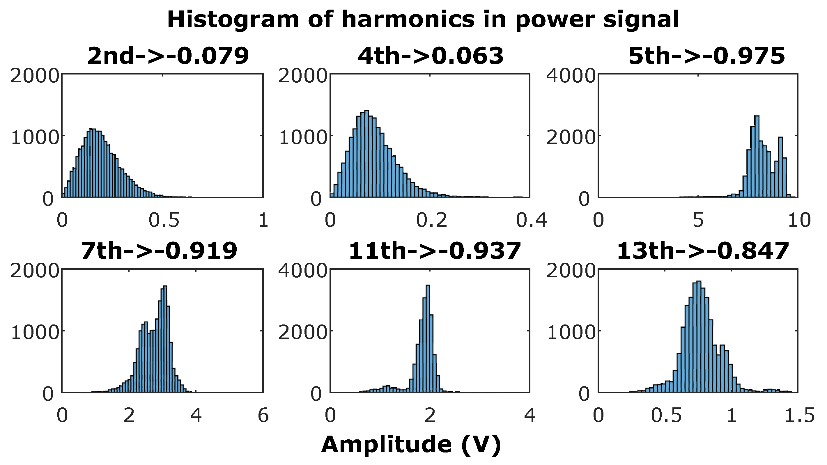
A histogram was calculated per each analyzed frequency in this case, but the fundamental frequency. In order to understand dispersion in relation to the mean value, histograms starting with zero amplitude were calculated. When this was done for fundamental frequency, all points were concentrated in a single bar (not depicted). Histograms for all other frequencies are plotted in Figure 13, with the associated SK value over each one.

As in the arc furnace signal analysis, components with an SK value near zero are associated with non-concentrated values. In fact, these were the second and fourth harmonics, related to noise, which showed random amplitude oscillations. Lower SK values were obtained as the amplitude values were more concentrated around the mean value. This can be observed in the thirteenth (SK value $-0.847$) and seventh harmonic (SK value $-0.919$), where the point distribution presented two tails, so there were few values higher or lower than the mean value. The eleventh harmonic (SK value $-0.937$) only showed one tail to lower values in the point distribution, so few points took lower values. The fifth harmonic (SK value of $-0.975$) showed a point distribution without tails, so points were concentrated around the mean value, but not enough to be considered a constant amplitude trend.

6. Conclusions

In this research work, an estimator for the SK is used in order to characterize amplitude variability in power systems’ spectra. More precisely, SK is studied to evaluate amplitude trends on each spectral component, focusing on the detection in constant amplitude trends.

The SK estimator shows flexible detection capacity, based on points’ concentration around the mean value, and not if only one value is outside the threshold, which can cause false detections. This implies a detection of a big amplitude change with a short length or a small amplitude change with a long length. In this way, if SK indicates a value very near $-1$, a constant amplitude trend is detected, due to really small amplitude changes being detected.

The relation among the SK value and the amplitude values’ dispersion, per each frequency component, is confirmed with two real-life signals. The first one is an electric current waveform form an arc furnace, taken at three different time periods of 40 s each. As the power level during the melting process is similar, the current level shows low variations. Amplitude value changes around the mean value are observed, and as postulated in this work, lower SK values are obtained when the amplitude values are more concentrated around the mean value. The second signal used is an hour of voltage signal taken from the power grid of the University of Cádiz. Even in a power system, with a nominal level, the amplitude value changes, and the 50-Hz frequency component shows low amplitude variations; it is set as a constant amplitude trend. SK analyzes each frequency component separately, so variations of each frequency component are only related to its mean value, allowing one to study in the same SK analysis frequency components with amplitude mean values greater than 100-times lower, in this case. In the study of these harmonics, it is confirmed again that points’ dispersion around the mean value is related to the SK value, giving lower SK values as the amplitude values are more concentrated around the mean value.

With all this, it is shown and confirmed that SK is a good tool to detect a constant amplitude trend, being able to return information beyond maximum variation around the mean value and giving a progressive index of value dispersion around the mean value, for each frequency component. In addition, as frequencies are studied separately, a signal that shows different amplitudes at different frequencies can be examined without any problem (e.g., voltage or current harmonics).