Article

Sample Entropy Based Net Load Tracing Dispatch of New Energy Power System

School of Electrical Engineering, Dalian University of Technology, Dalian 116024, China
*
Author to whom correspondence should be addressed.
Energies 2019, 12(1), 193; https://doi.org/10.3390/en12010193
Submission received: 18 November 2018 / Revised: 25 December 2018 / Accepted: 7 January 2019 / Published: 8 January 2019

Abstract

:
The high-proportion of renewable energies is gradually becoming one of the main power supply sources and bringing strong uncertainties to the power grid. In this paper, a sample entropy (SampEn) based net load tracing dispatch strategy with a specific thermal generating mode is proposed. In this strategy, renewable energies are fully and preferentially consumed by electric loads, turned to net loads, to maximize the utilization of renewable energies. SampEn theory is utilized to evaluate the complexity of net load time series, based on which, the traditional power generators trace the complexity of the net load flexibly. According to the SampEn, a specific generating model of thermal generators is determined and the cooperation between thermal generators and pumped storage is realized, aiming at reducing the ramp power of thermal generators and increasing the throughput of pumped storage. The experiment simulation is developed on the 10-unit test system. Results show that the ramping power of the thermal generators are reduced 43% and 13% in the two cases together with the throughput of pumped storage is increased 44% and 27% on the premise that the economy of the system is maintained and renewable energies are fully consumed. Therefore, the efficiency and reasonability of the proposed dispatch strategy are confirmed.

1. Introduction

The modern power system is transforming to the third-generation power system, or called new energy power system, which mainly depends on those clean and renewable non-fossil energies [1], such as wind power [2], solar energy [3], and so forth. In the new energy power system, the intermittent energies such as wind power and photovoltaic share the responsibility of power load demand together with the traditional power sources. The thermal power output in the traditional day-ahead power dispatch with high uncertainties will ramp up and down frequently. Thus, the inlet valve of steam turbine will be adjusted accordingly, which will lead to the difficulties on actual operation and the aggravation of mechanical wear [4,5]. In the long run, the power generation efficiency will be decreased and the life of the generators will be shortened. Therefore, the reasonable determination of unit generating mode, which can not only respond to these strong uncertainties, but reduce the power output fluctuation and increase the utilization efficiency of non-fossil energies as well, plays an important role in the new power system dispatch.
The renewable energies with high proportion have gradually been as important as traditional power sources and the proportion is expected to reach up to 60% by 2050 [6]. Moreover, the distributed generators, electric vehicles, energy storages and so forth on the load side increase the uncertainties of the system as well. Hence, researchers introduced the concept of net load [7,8]. The net load means the imbalance between electric loads and intermittent power energies. In this way, the source–load bilateral uncertainty problem is transformed to how to respond to the uncertainty of net loads.
There are many studies focusing on the power balancing problems related to high-proportion renewable energies connected to the power grid. The multi-source coordination of power systems is an effective means. The flexible resources such as hydropower plant, gas turbine power plant, energy storage, and so forth are developed and utilized to respond to the uncertainty and fluctuation of renewable energies cooperatively [9,10]. In [10], a robust unit commitment model considering the cooperation of wind power and pumped storage is proposed, in which the wind power fluctuation is restrained by the pumped storage. Reference [11] utilized the second life battery energy storage to assist thermal generators to respond to the fluctuation of renewable energies. Facing the high-percentage renewable energies, the ramp capability of generators is an important factor when to response to the load demands [12,13,14]. It is argued in [15] that the insufficient ramp resources in the system may lead to the insufficient flexibility to meet variations in the net loads. Reference [16] estimated the potential variability of net loads by the statistical approaches on the ramping characteristics to determine the required ramping capability in the future. The increasing ramping capability can improve the flexibility on supply side. However, the above studies are based on the traditional power dispatch. With the increasing of renewable energies percentage, the amplitude and frequency of generating and ramping power adjustments are still increased, which will cause security risks of system operation. Power dispatch contains different time-scales. The horizon optimization of day-ahead power dispatch is 24 h [17,18]. The advance dispatch operates in the framework of a short time, such as 30 min [17]. The shorter time-scale can be state estimation, which contains load power measurement, estimation, and dispatching [19,20,21,22,23]. In order to deal with the problems of renewable energies connected to the power grid and the ramping constraints of generators, there are studies focusing on the dispatch from the perspective of time dimension. Reference [24] proposes a model considering operational flexibility at sub-hourly time-scales. Reference [25] provides a multi-time scale coordination power dispatch divided into day-ahead, intra-day, and real-time scale. Reference [26] studies a unit commitment strategy aiming at improving the ramping capability of generators. The strategy provides multiple time-scale ramping constraints to satisfy the demand of load prediction, in which the ramping capability can cover the whole varies range of the uncertain renewable energies. However, sufficient ramping reserve will lead to wasting of resources.
Besides, the description method of net load uncertainties affects the determination of dispatch strategy. The uncertainty characteristics of supply side and load side can be described and analyzed respectively [27,28] further to stabilize the uncertainty of net loads. The stochastic programming model [29] or fuzzy program model [27,30] of the net loads are built and solved by fitting optimization methods, such as the sample-based stochastic decomposition approach [31] and the Benders decomposition method [32]. In [33], the Fourier transform is applied to calculate the convolution of load and wind power and compute the probability distribution of joint variables. These studies, however, are still focused on the assumption and simulation of the distribution characteristics of the power and loads. There is not much attention on numeric characteristics analysis. Reference [34] analyzed the duration curves, volatility, and hourly ramps of net loads and indicated that the characteristic of net loads plays an important role in the power grids with high penetration of renewables. The uncertainty and disorder of net load can be analyzed and measured by the concept of entropy [35,36,37]. The approximate entropy can be utilized to analyze the characteristics of data and evaluate the complexity level of the time series, and it is widely used in many fields [38]. However, the consistency of approximate entropy is poor and during the solution process, there are self-data comparisons and deviations. These weaknesses promote the utilization of sample entropy (SampEn) developed by Richman [39,40], which has better applicability and can evaluate the complexity level more accurately [41,42].
In this paper, a sample entropy based net load tracing dispatch strategy with a specific thermal generating mode is provided to increase the operation efficiency of thermal generators and the stability of the system in the premise that the economy of the system is ensured. In order to make full use of the renewable energy, wind power and photovoltaic power are consumed by electric loads first, turned to net loads. Focusing on the day-ahead power dispatch, the SampEn theory is used to evaluate the complexity level of net loads. On these bases, the traditional dispatch is transformed to a specific generating mode according to the SampEn, in which the thermal ramping mode and time duration are determined. The high operation efficiency and less ramping power of thermal generators are achieved. Moreover, the high throughput of pumped storage is realized. A simulation model based on a 10-unit power system is developed and tested in MATLAB (R2018a, MathWorks, Natick, MA, USA).
This paper is organized as follows. Section 2 analyzed the characteristics of the net loads and introduced the SampEn calculation of net loads. In Section 3, a net load tracing dispatch strategy based on SampEn is studied in detail. The case study and discussion are conducted in Section 4. Finally, the conclusions are stated in Section 5.

2. Characteristics of Net Loads and SampEn Calculation

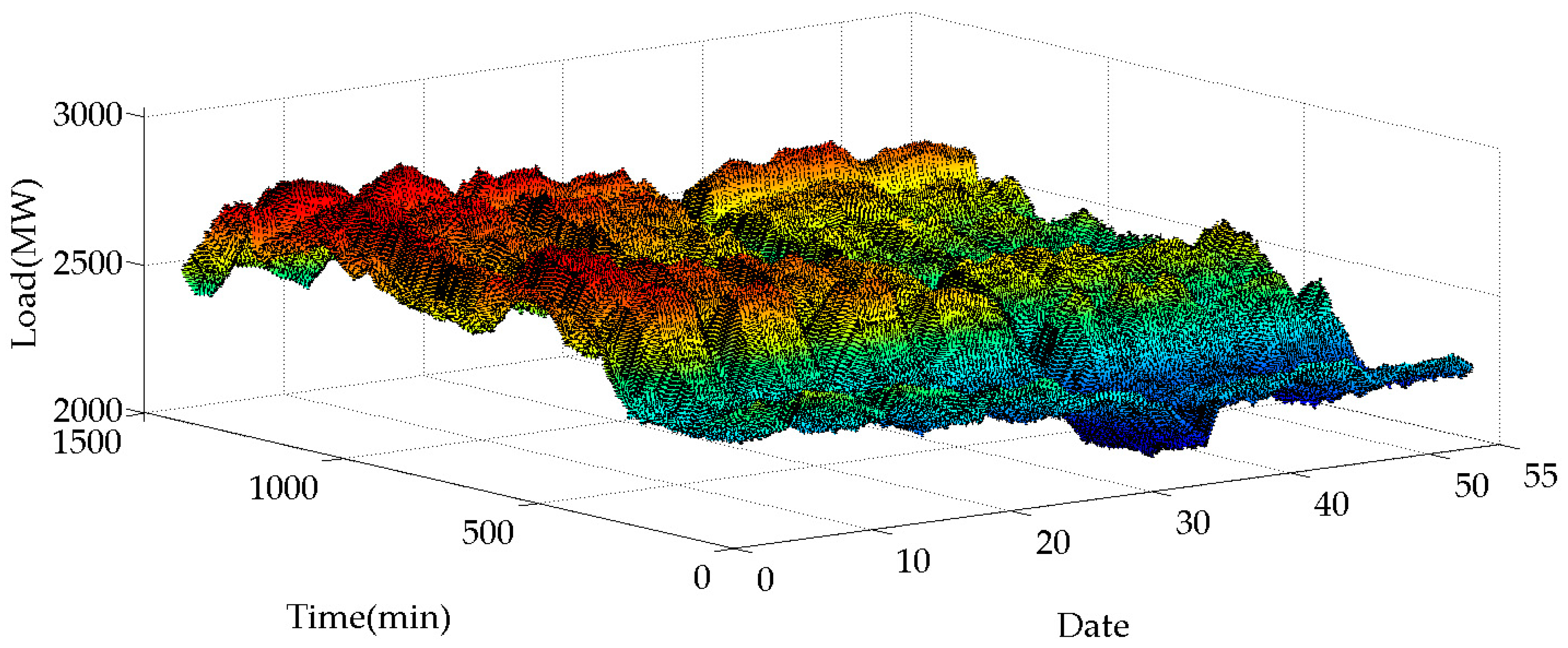
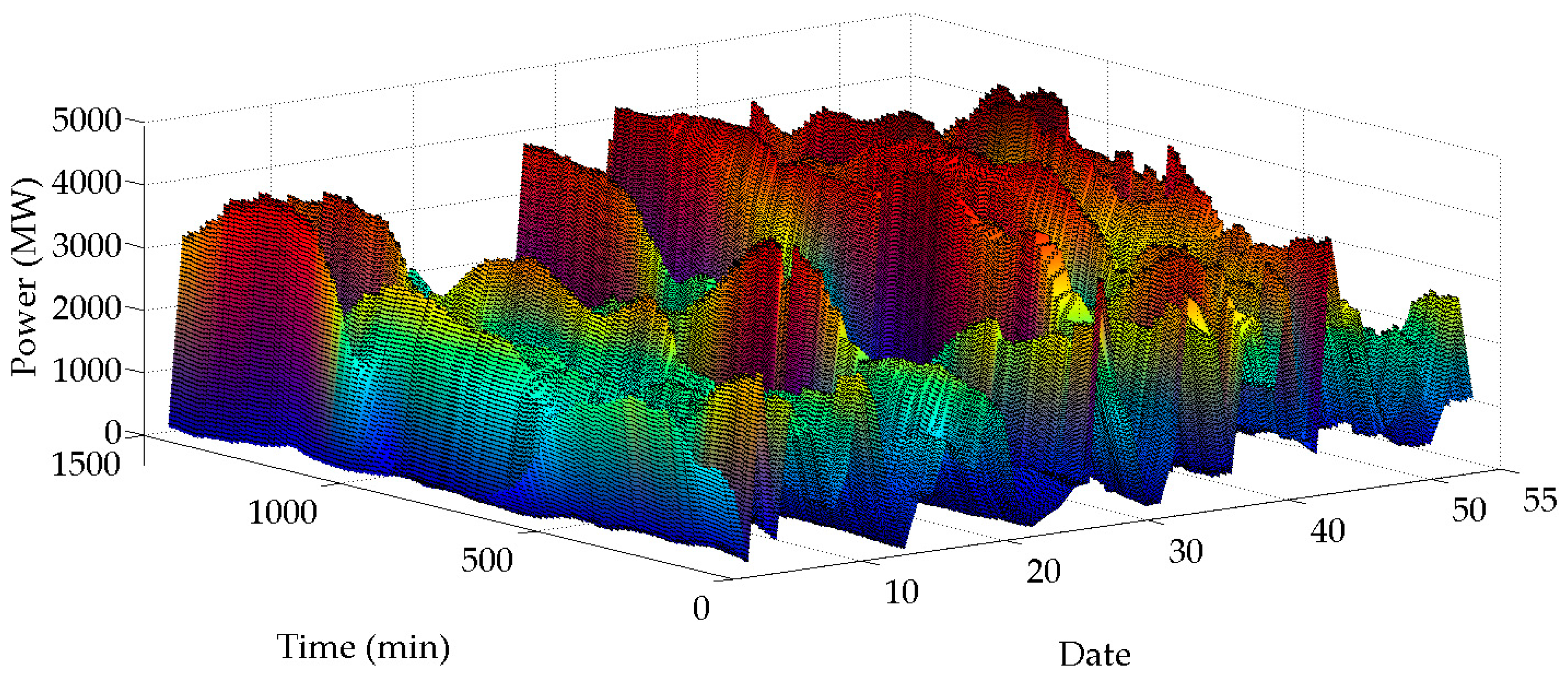
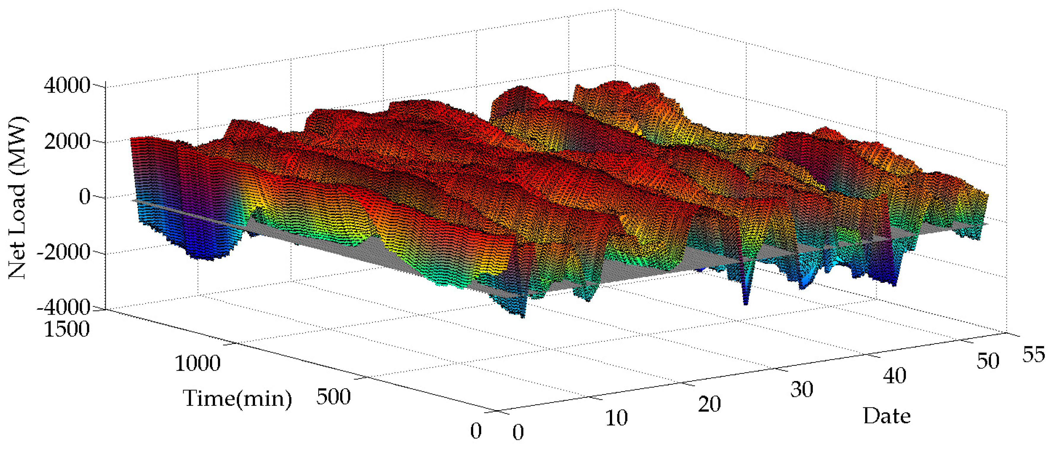
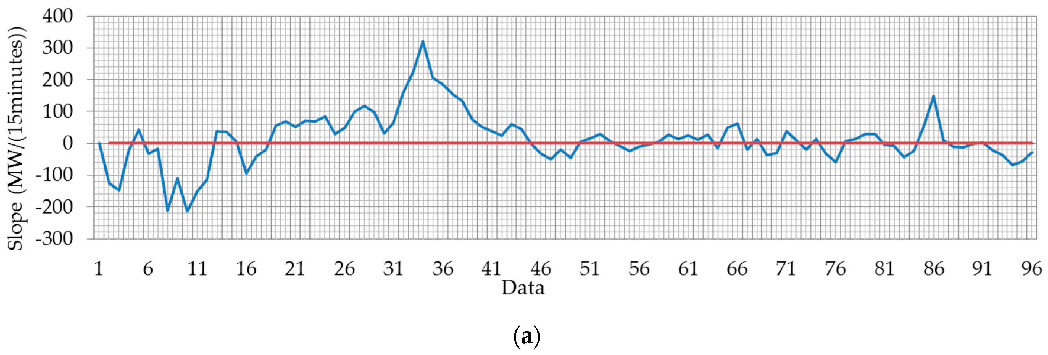
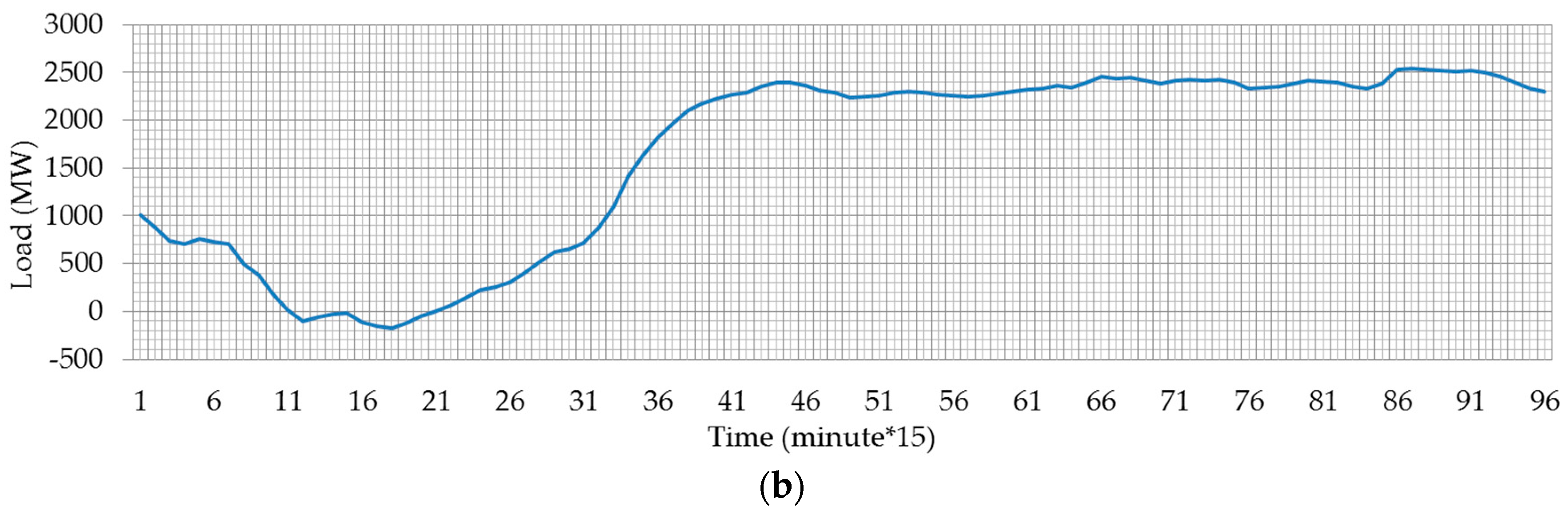
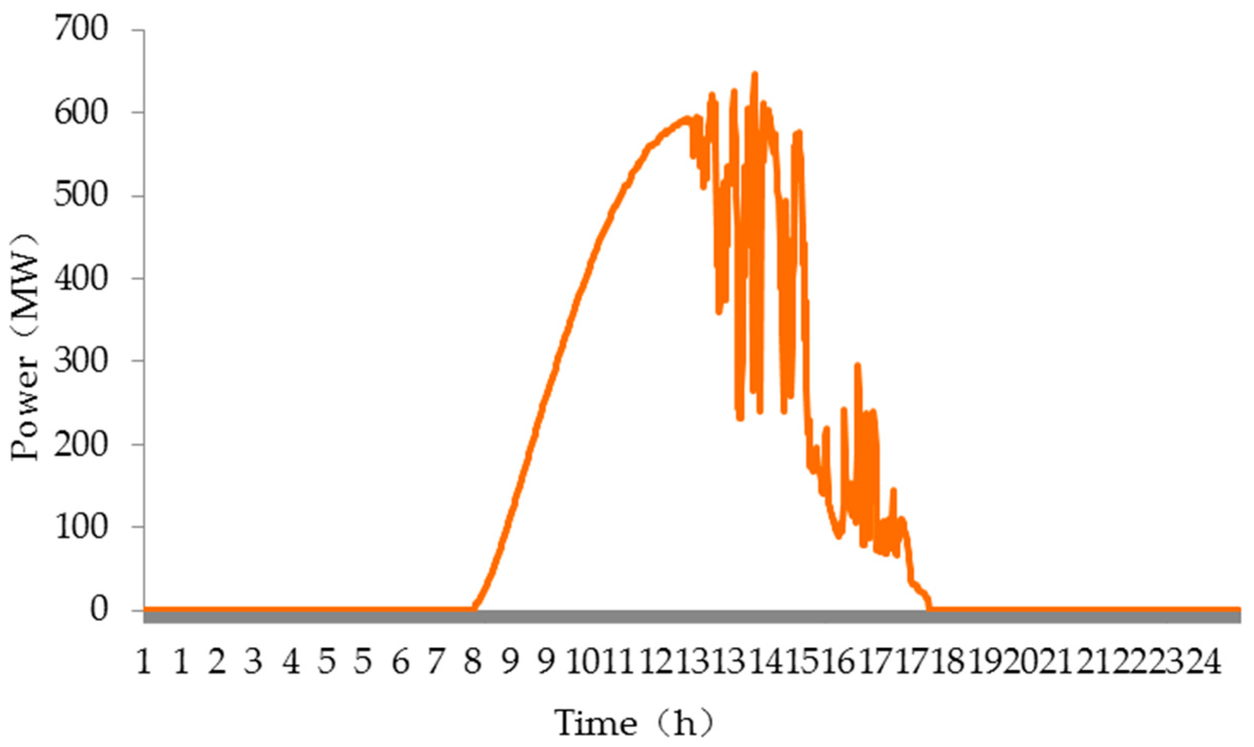
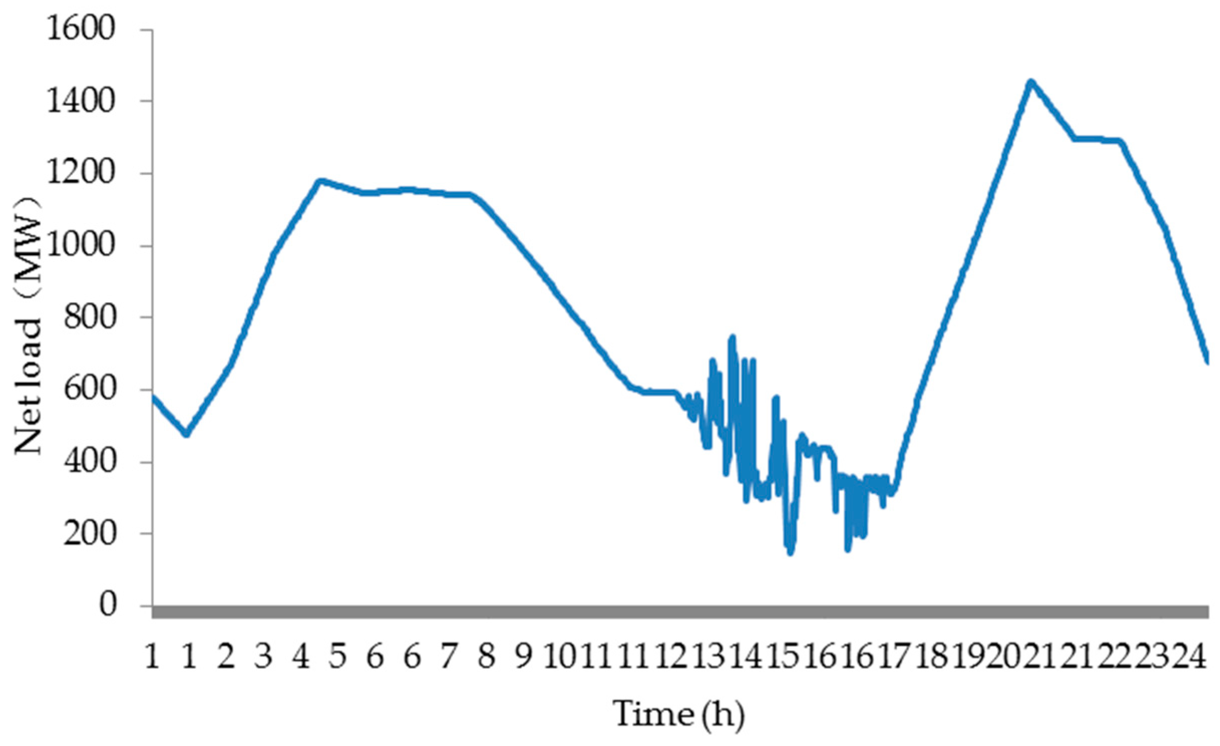
2.1. Net Loads Description

The variation of load data and wind power in a specific province from 3 March to 24 April 2017 are shown in Figure 1 and Figure 2, respectively. Based on those data, the electric loads are 12.5% scale-down to match the wind data for simulating a power grid operation condition with high-percentage wind power. After the scale-down, the trend of curve remains unchanged and the differences between wind power and electric loads are defined as net loads shown in Figure 3. As shown in Figure 3, the net loads are highly stochastic. No obvious regulation or trend can be found in these figures. If the power dispatch strategies remain the traditional ones, such highly stochastic net loads will result in large fluctuations on the power supply side, causing thermal generation power outputs to change frequently and decrease the efficiency and stability of the system.
This paper focuses on the dispatch on the net loads with strong uncertainty and large fluctuation. The time series is used to describe the net loads and the SampEn is utilized to evaluate the complexity level of the net loads.

2.2. SampEn of Net Loads in New Energy Power System

According to the theory of SampEn, the value of SampEn is positive correlation to the complexity level of sample series. That is, the time series with larger SampEn value are more complicated than the one with lower SampEn value. The calculation of SampEn does not include the comparison of its own data series. Therefore, the calculation is independent to the length of the series. The comparison of two time series will still be the same in any of their subsequence dimension and with similar tolerance level. In addition, the SampEn calculation can remain unaffected with over one-third data loss [43].
In the theory of SampEn, the complexity means the generation rate of new data mode with time. In a time series with larger SampEn, new data modes will be generated with higher frequently and vice versa [44]. By defining the sign change of the slope as the new mode, the generation rate of new mode is reflected through the polarity changing frequency of the slope. The change of slope sign indicates the direction of the net load variation has been altered. The changing frequency of the slope sign reflects not only the changing speed of value but also the changing speed of changing direction. On the contrary, if the slope signs are not changed in a time period, the net loads will be changed monotonously or limited changes in direction can be found. In this paper, the slope of the adjacent points, the changing rate of the slope sign and the valley-to-peak of the time series are calculated and analyzed. Through the rolling calculation of the SampEn and its auxiliary value of the time series, the corresponding scheduling period is divided and the strategy of the dispatch are confirmed.
Based on the description above, the computational procedure of the S a m p E n N e t L o a d of the net load time series is shown as follows:
1. The whole net load time series is given: { N L l } = { n l ( 1 ) , n l ( 2 ) , , n l ( N ) } , where the N is the total amount of states;
2. The slope of the adjacent points in net load { N L l } is shown in Equation (1).
S l o p e ( l ) = n l ( l + 1 ) n l ( l )
where, l = 1 , 2 , , N 1 ;
3. The slope signs are calculated as Equation (2) shows and the changing markers are determined as Equation (3) shows.
s y m b o l l S l o p e = sign ( S l o p e ( l ) )
{ i f s y m b o l l S l o p e = s y m b o l l + 1 S l o p e , t r a n s l S l o p e = 0 i f s y m b o l l S l o p e s y m b o l l + 1 S l o p e , t r a n s l S l o p e = 1
4. The ratio of sign changing amount to net load amount is rolling calculated during the time t l ~ t l + k . The equation is shown as
R a t i o l , l + k S l o p e = count k = 1 ~ N l + 1 ( t r a n s l S l o p e ,   t r a n s l + k S l o p e ) k
5. The ratio of R a t i o l , l + k S l o p e to the valley-to-peak of the net loads S u p l , l + k S a m p E n is rolling calculated during the time t l ~ t l + k . The calculated value is as the auxiliary value of the net load time series. The equation is shown in (5).
S u p l , l + k S a m p E n = R a t i o l , l + k S l o p e max k = 1 ~ N l + 1 ( n l ( l ) , n l ( l + k ) ) min k = 1 ~ N l + 1 ( n l ( l ) , n l ( l + k ) )
The piecewise estimation of the net load series is conducted based the S u p l , l + k S a m p E n . The similar S u p l , l + k S a m p E n are divided in the same time period, and the piecewise time points t g , g N are achieved. Thus, the subsequence of net load is expressed as { n l ( g ) , n l ( g + 1 ) , , n l ( g + T N L ) } , where T N L is the length of the net load subsequence.
6. The time series { P i N e t L o a d } = { p N L ( 1 ) , p N L ( 2 ) , , p N L ( T N L ) } is assumed as the subsequence of the net load at time t g . A subsequence with dimension of m N L is generated as Equation (6) shows
P N L ( i ) = [ p N L ( i ) , p N L ( i + 1 ) , , p N L ( i + m N L 1 ) ]
where, i = 1 , 2 , , T N L m N L + 1 and m N L is usually equal to 2 or 3.
7. The D N L i j     m N L ( P N L ( i ) , P N L ( j ) ) is defined as the distance of the subsequence P N L ( i ) and P N L ( j ) , where j = 1 , 2 , , T N L m N L + 1 , j i . The distance means the maximum value of the difference between the corresponding elements in these two subsequences. To each i the distance between P N L ( i ) and P N L ( j ) is shown in Equation (7).
d i j m N L ( P N L ( i ) , P N L ( j ) ) = [ | u ( i ) u ( j ) | | u ( i + 1 ) u ( j + 1 ) | | u ( i + m N L 1 ) u ( j + m N L 1 ) | ]
Thus, the distance of the subsequence P N L ( i ) and P N L ( j ) is calculated as Equation (8) shows.
D N L i j     m N L ( P N L ( i ) , P N L ( j ) ) = max ( d i m N L ( P N L ( i ) , P N L ( j ) ) )
8. The tolerance level r N L is a threshold defining when two states are similar, where r N L > 0 . In this paper, the r N L was set 0.2 × S T D N L , S T D N L is the standard deviation of N L . To each i, the amount of D N L i j     m N L ( P N L ( i ) , P N L ( j ) ) < r N L are calculated. B N L i m N L ( r N L ) is defined as Equation (9):
B N L i m N L ( r N L ) = count ( D N L i j     m N L ( P N L ( i ) , P N L ( j ) ) < r N L ) T N L m N L
where T N L m N L is the total distance of the sample.
9. The actual average over all the vectors B N L i m N L ( r N L ) of is computed as Equation (10) shows.
B A v g m N L ( r N L ) = i = 1 T N L m N L + 1 B N L i m N L ( r N L ) T N L m N L + 1
10. The dimension of subsequence is increased to m + 1. Repeat steps 6 to 10 and achieve B A v g m N L + 1 ( r N L ) . Theoretically, the sample entropy is defined as
S a m p E n N e t L o a d ( r N L , m N L ) = lim T N L { ln ( B A v g m N L + 1 ( r N L ) B A v g m N L ( r N L ) ) }
In practice, the length of time series T N L is finite. Therefore, the estimation of SampEn is denoted as Equation (12).
S a m p E n N e t L o a d ( r N L , m N L , T N L ) = ln ( B A v g m N L + 1 ( r N L ) / B A v g m N L ( r N L ) )

2.3. SampEn Application of Net Loads

The net load data of a province on 3 March and 4 April are shown in Table 1. The net load curve and the adjacent point slope of 11 April and 3 March are shown in Figure 4 and Figure 5, respectively. According to the calculation process of SampEn in Section 2.2, the subsequence series are divided into different time length and calculated correspondingly. As Table 1 shows, the ratio of slope sign changing frequency to valley-to-peak is proportional to the SampEn, which also can be verified by Figure 4 and Figure 5.
The data in time interval of 1 to 18 and 42 to 69 in Figure 4 show that the slope sign of adjacent points change frequently while the ratio of slope sign changing amount to valley-to-peak stays large. Thus, the curve fluctuates irregularly in a small range and the corresponding SampEn is large. The above result analysis is also suitable for the data in time interval 46 to 96 in Figure 5.
In addition, the data in time interval of 19 to 41 and 70 to 96 in Figure 4 show that the slope sign of adjacent points changing amount are less and the ratio of slope sign changing amount to valley-to-peak is small. Thus, the curve appears to monotonic variation in a certain time period and only a single or small numbers of sharply data changes and changing tendency can be found. The complexity level of the subsequence is low and the corresponding SampEn is small. The above result analysis is also suitable for the data in time intervals 1 to 45 in Figure 5.

3. New Energy Net Load Tracing Dispatch Strategy Based on SampEn

3.1. Generating Mode of Thermal Generators

The complexity level of the net loads can be reflected by SampEn. The net load with larger SampEn will be at a higher complexity level. In a certain time periods, the data of net loads change frequently and there is no obviously data increase or decrease. Thus, the power outputs of thermal generators prefer to remain constant and the pumped storage is as the main supply power source. On the contrary, the net load with lower SampEn will be at a lower complexity level. In certain time periods, there are obviously increase and decrease of the net loads. In addition, the variations will last periods of time. Although the pumped storage is available to respond to the increase and decrease of the net loads, the power outputs cannot last for a long time. Thus, the thermal generators and the pumped storage are in cooperation as the main supply power sources.
The generating mode of thermal generators based on SampEn is determined as follows:
The SampEn S a m p E n t g t l N e t L o a d of net load series P N L t g t l in time periods t g to t l is calculated as Section 2.2 shows. The generating mode setting is depended on the value of S a m p E n t g t l N e t L o a d . If S a m p E n t g t l N e t L o a d is large, the complexity level in this time period is high and the fluctuation of thermal generation are minimized. If S a m p E n t g t l N e t L o a d is small, the complexity level in this time period is low and the thermal generators are operated normally to response to the net loads. The generating mode is settled as Equation (13) shows.
{ S a m p E n t g t l N e t L o a d   i s   b i g : | max [ P p i , t g : P p i , t l ] min [ P p i , t g : P p i , t l ] | S a m p E n t g t l N e t L o a d S a m p E n t g t l N e t L o a d   i s   s m a l l : P p i min P p i , t P p i max ( t g ,   t l t )
where P p i , t is the real power output of unit pi at time t. P p i min and P p i max are the minimum and maximum power outputs of the ith thermal generator, respectively.

3.2. Power Dispatch Model Based on SampEn

3.2.1. Objective Functions

The thermal generation cost F t h e r m a l is considered as the objective function in this paper, which is calculated by
F t h e r m a l = t = 1 T p i n g ( a p i × P p i , t 2 + b p i × P p i , t + c p i )
where T is total number of time periods; ng is the number of dispatchable units; a p i , b p i , and c p i are the coefficients of fuel cost functions for units pi.

3.2.2. Power Balance Equations and Constraint Functions

1. Power Balance Equations
The power balance equations at time t are formulated as
p i = 1 n g P p i , t + H g e n i = 1 n p P H g e n i , t - P N L t H p u m p i = 1 n p P H p u m p i , t = 0
P N L t = P L t w p i = 1 n w P w p i , t p r e s o l a r i = 1 n s P s o l a r i , t p r e
where p i = 1 n g P p i , t is the total generator power output during the tth time period; P L t is the total load demand at time t. P H g e n i , t is the generating power of pumped storage H g e n i at time t and P H p u m p i , t is the pumping power of pumped storage H p u m p i at time t. P N L t is the total net load demands at time t. P w p i , t p r e is the predicted wind power of wind farm wpi at time t and P s o l a r i , t p r e is the predicted photovoltaic power of photovoltaic station solari at time t. n p , n w , and n s are the total number of the pumped storage, wind farms, and photovoltaic power stations, respectively.
2. The constraints of pumped storage
The pump and generating power constraints of pumped storage are shown in Equations (17) and (18).
P H g e n i min P H g e n i , t P H g e n i max
P H p u m p i min P H p u m p i , t P H p u m p i max
where P H g e n i min and P H g e n i max are the minimum and maximum generating power of pumped storage H g e n i , respectively. P H p u m p i min and P H p u m p i max are the minimum and maximum pumping power of pumped storage H p u m p i , respectively. The constraints of the reservoir energy conversion are shown as follows:
H P u m p i , t + 1 = H P u m p i , t + Δ t × ( P H p u m p i , t × γ P u m p P H g e n i , t γ G e n )
H P u m p i min H P u m p i , t H P u m p i max
where H P u m p i , t + 1 and H P u m p i , t are the storage condition of the reservoir at time t + 1 and time t. Δ t is the time interval. γ P u m p is the pumping efficiency and γ G e n is the generating efficiency. H P u m p i min and H P u m p i max the minimum and maximum power storage of reservoir. Moreover, the pumping and generating processes of the pumped storage cannot be carried out at the same time, which is as Equation (21) shows.
P H g e n i , t · P H p u m p i , t = 0
3. Constraints of Thermal Generators
The power output constraints of thermal generators are shown in Equation (22).
P p i min P p i , t P p i max
The generating ramp rate limits are formulated by
{ P p i , t P p i , t 1 U R p i P p i , t 1 P p i , t D R p i
where U R p i and D R p i are the ramp-up and ramp-down rate limits of the ith thermal generator, respectively.
The spinning reserve chance constraints are formulated by Equations (24) and (25). The up and down reserve should cover the errors between the actual wind power output and the predicted wind power output. In order to avoid the waste of reserve sources, the reserve needs not to cover the whole error range and only to satisfy a certain probability. In addition, the upper limits of up and down reserve are shown in Equations (26) and (27).
Pr { p i = 1 n g P U R i , t w p i = 1 n w ( P w p i , t p r e P w p i , t ) } ρ
Pr { p i = 1 n g P D R i , t i = 1 n w ( P w p i , t P w p i , t p r e ) } ρ
P U R i , t min ( P p i max P p i , t , U R p i )
P D R i , t min ( P p i , t P p i min , D R p i )
where ρ is the confidence coefficient and P w p i , t is the actual wind power of wind farm wpi at time t. P U R i , t and P D R i , t are the actual up and down reserve of thermal generator pi.

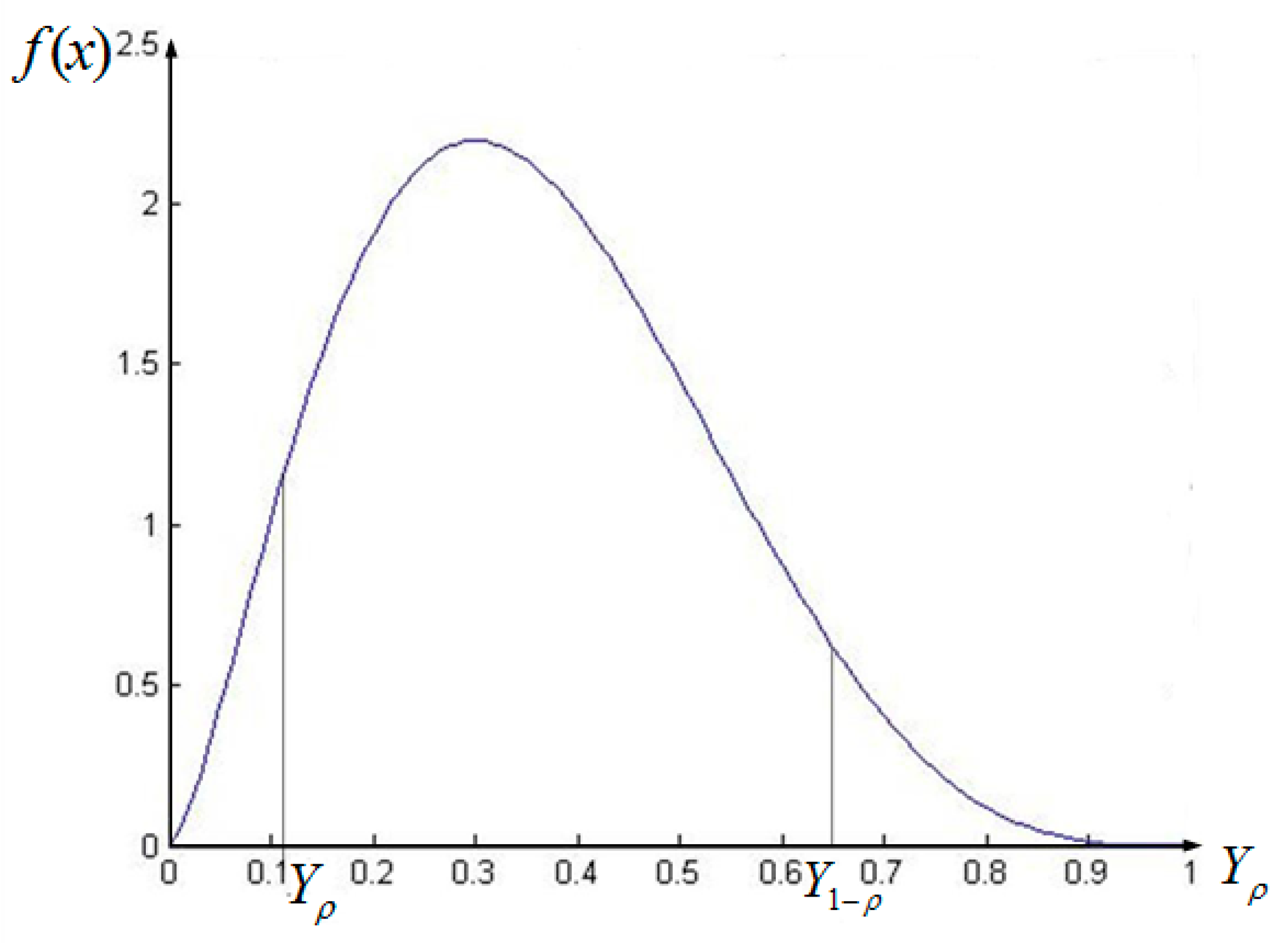
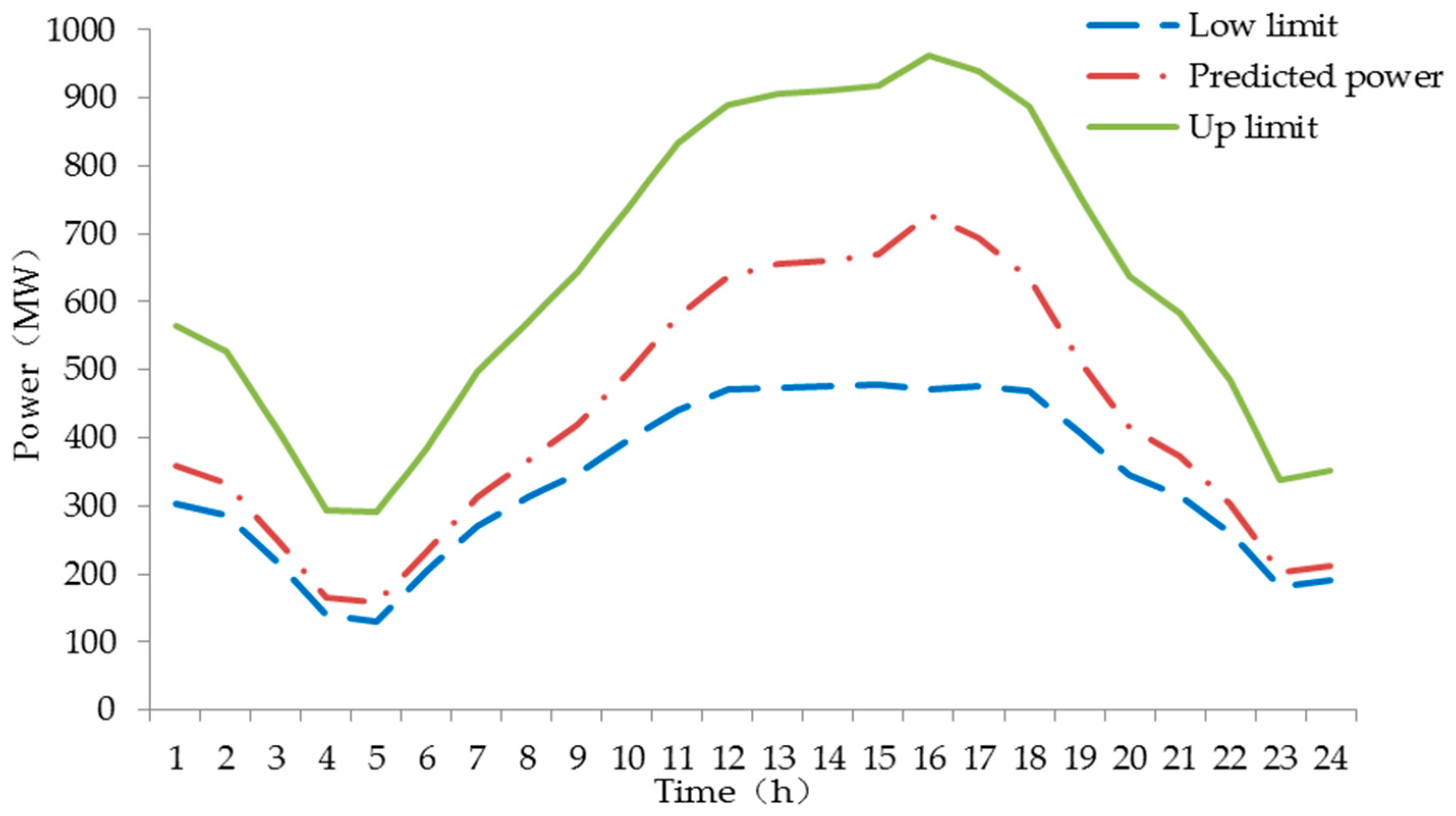
3.2.3. Stochastic Variables

The probability distribution of wind power is estimated based on the Beta distribution [45] and shown in Figure 6, which is described by
f w ( p w p ) = p w p α 1 ( 1 p w p ) β 1 B ( α , β )
where p w p is a normalized wind power output, B ( α , β ) is the Beta distribution function and α , β are the distribution shape parameters. The calculated formulas are
p w p = P w p P w p min P w p max P w p min , p w p [ 0 , 1 ]
B ( α , β ) = 0 1 p w p α 1 × ( 1 p w p ) β 1 d p w p
E ( p w p p r e ) = E ( P w p p r e P w p max ) = α α + β
D ( p w p p r e ) = D ( P w p p r e P w p max ) = α β ( α + β ) 2 ( α + β + 1 )
where P w p is the actual wind power output; P w p min and P w p max are the minimum and maximum outputs of wind turbines, respectively. P w p p r e is the predicted wind power; E ( p w p p r e ) is the expectation of P w p p r e ; and D ( p w p p r e ) is the variance of P w p p r e .
The fractile is used to solve the above chance constraints [46].
Pr ( Y > Y ρ ) = ρ ρ ( 0 , 1 )
where Y is the random variable and Y ρ is the fractile of ρ . In Figure 6, the Y ρ is the upper fractile and the Y 1 ρ is the lower fractile. f ( Y ) is the density function of Y. Equations (24) and (25) can be transformed into Equations (34) and (35), corresponding to the type of Equation (33). When the ρ is determined, the Y ρ and Y 1 ρ can be received by calculating the inverse function through MATLAB. Thus, when the function (36) is satisfied, the constraint (34) is ensured. When the function (37) is satisfied, the constraint (35) is ensured.
Pr { w p i = 1 n w P w p i , t p i = 1 n g P U R i , t + w p i = 1 n w P w p i , t p r e } ρ
Pr { w p i = 1 n w P w p i , t p i = 1 n g P D R i , t + w p i = 1 n w P w p i , t p r e } ρ
p i = 1 n g P U R i , t + w p i = 1 n w P w p i , t p r e w p i = 1 n w Y ρ i
p i = 1 n g P D R i , t + w p i = 1 n w P w p i , t p r e w p i = 1 n w Y 1 ρ i

3.3. Power Dispatch Strategy Process Based On SampEn

The power dispatch strategy is mainly divided in five parts:
1. Renewable energy is connected to the power grid and consumed by electric loads firstly. Thus, the net load time series is generated.
2. The characteristics and numeric features of the net loads containing the slope of the adjacent points shown in Equation (1), the total number of slope sign changes, ratio of sign changing amount to net load amount shown in Equation (4) and the ratio of proportion to the valley-to-peak of the net loads shown in Equation (5) are analyzed.
3. The characteristics of net load mentioned in Step 2 are rolling calculated. According to the results of S a m p E n t g t l N e t L o a d , the closer results are divided into one subsequence. Thus, the net load time series are divided into a few certain subsequences.
4. The SampEn of the subsequences are calculated and the time frame is determined according to the point-in-time of the subsequences. Moreover, the generating mode of thermal generators is confirmed according to the SampEn as Equation (13) shows.
5. The power dispatch strategy based on SampEn is conducted. A prime-dual interior point method is used to solve the optimization problem.
The flow chart of the power dispatch strategy is shown in Figure 7.

4. Case Study

In order to demonstrate the effectiveness of the proposed power dispatch strategy, a 10-unit test system [47] is developed in this work. The unit data and cost coefficients are modified from [47,48] and listed in Table 2, where P max and P min are the maximum and minimum power limit of the units, respectively; a, b, and c are the coefficients of fuel cost functions for units; UR and DR are the ramp-up and ramp-down rate limits of the units, respectively; C o e U R i and C o e D R i are the up and down reserve cost coefficients, respectively; C o e r a m p u p i and C o e r a m p d o w n i are the up and down ramping cost coefficients, respectively. The load demand changing curve is shown in Figure 8, and the maximum load is 2220 MW. The installed capacity of pumped storage is 700 MW and the total available operational thermal power is 2358 MW. There are two wind farms with 500 MW installed capacity, respectively and the wind power penetration is 45%. The predicted wind power curves and the limit curves are shown in Figure 9. The installed capacity of photovoltaic station is 600 MW and the penetration is 27% as shown in Figure 10. The percentage of renewable energy in this model is 72% and the net load curve is shown in Figure 11.

4.1. SampEn Calculation

The characteristics and numeric features of the net loads are analyzed and the SampEn are calculated. The results are shown in Table 3.

4.2. Result Comparison and Analysis of Cases

The simulation in this paper is conducted in four cases.
  • Case 1: power dispatch without SampEn and the wind power reserve confidence degree is 0.9.
  • Case 2: power dispatch based on SampEn at wind power reserve confidence degree of 0.9.
  • Case 3: power dispatch without SampEn and the wind power reserve confidence degree is 0.95.
  • Case 4: power dispatch based on SampEn at wind power reserve confidence degree of 0.95.

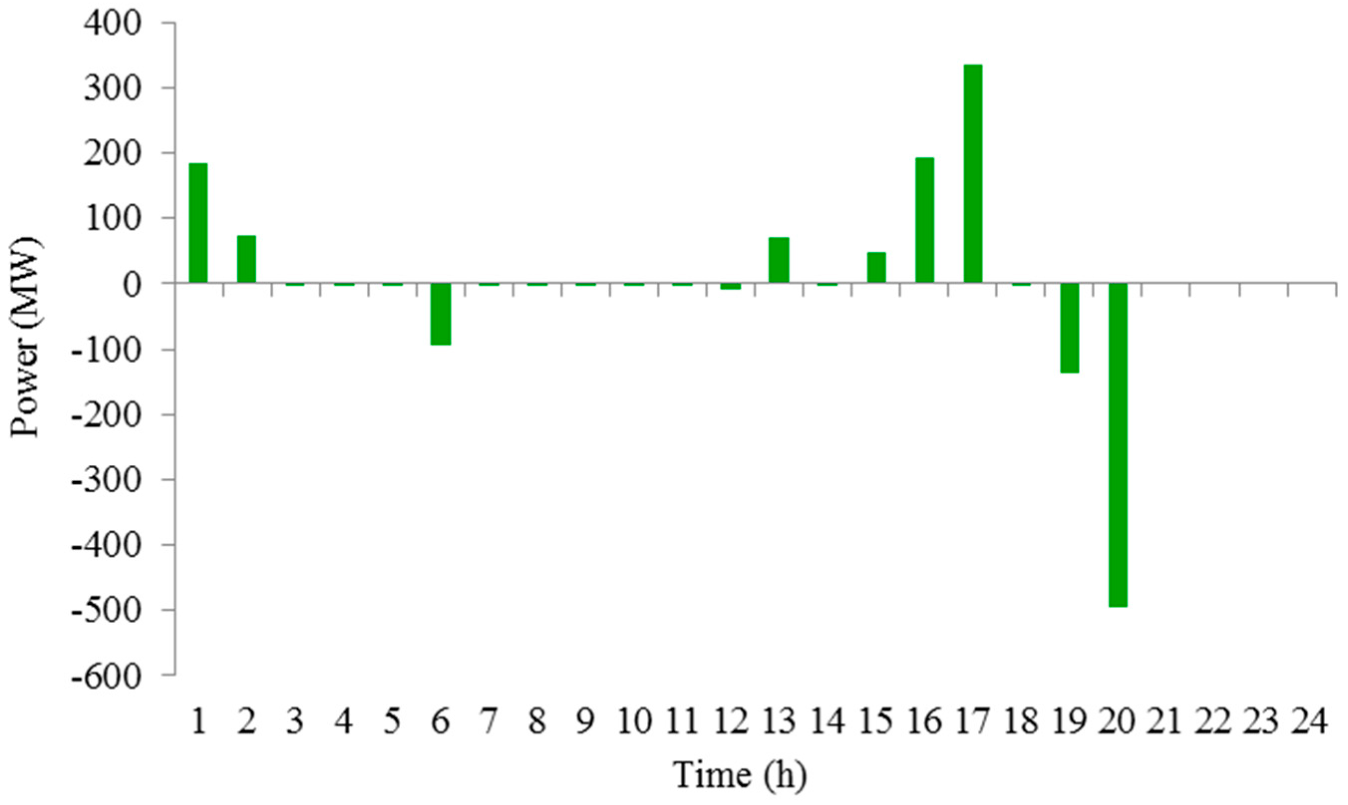
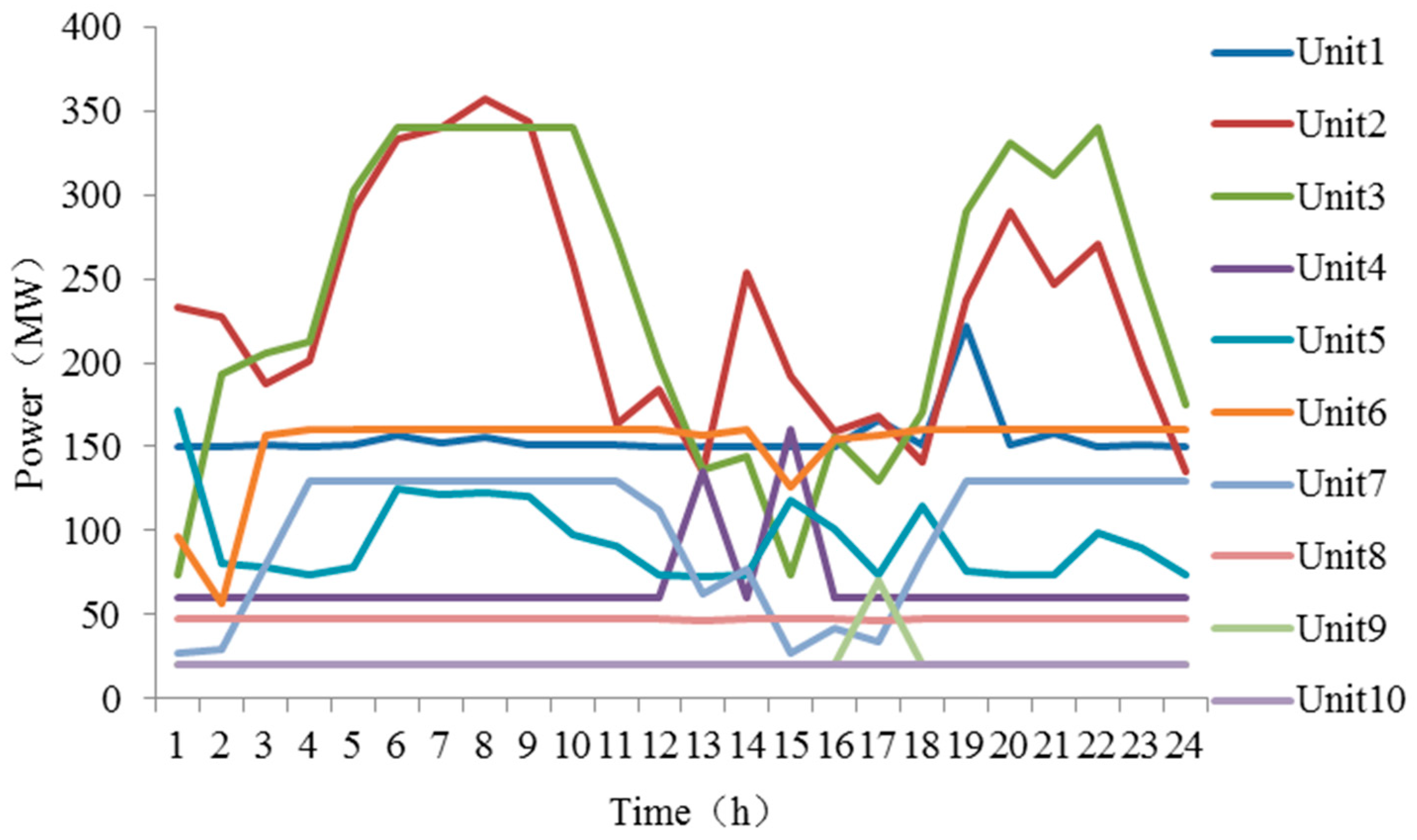
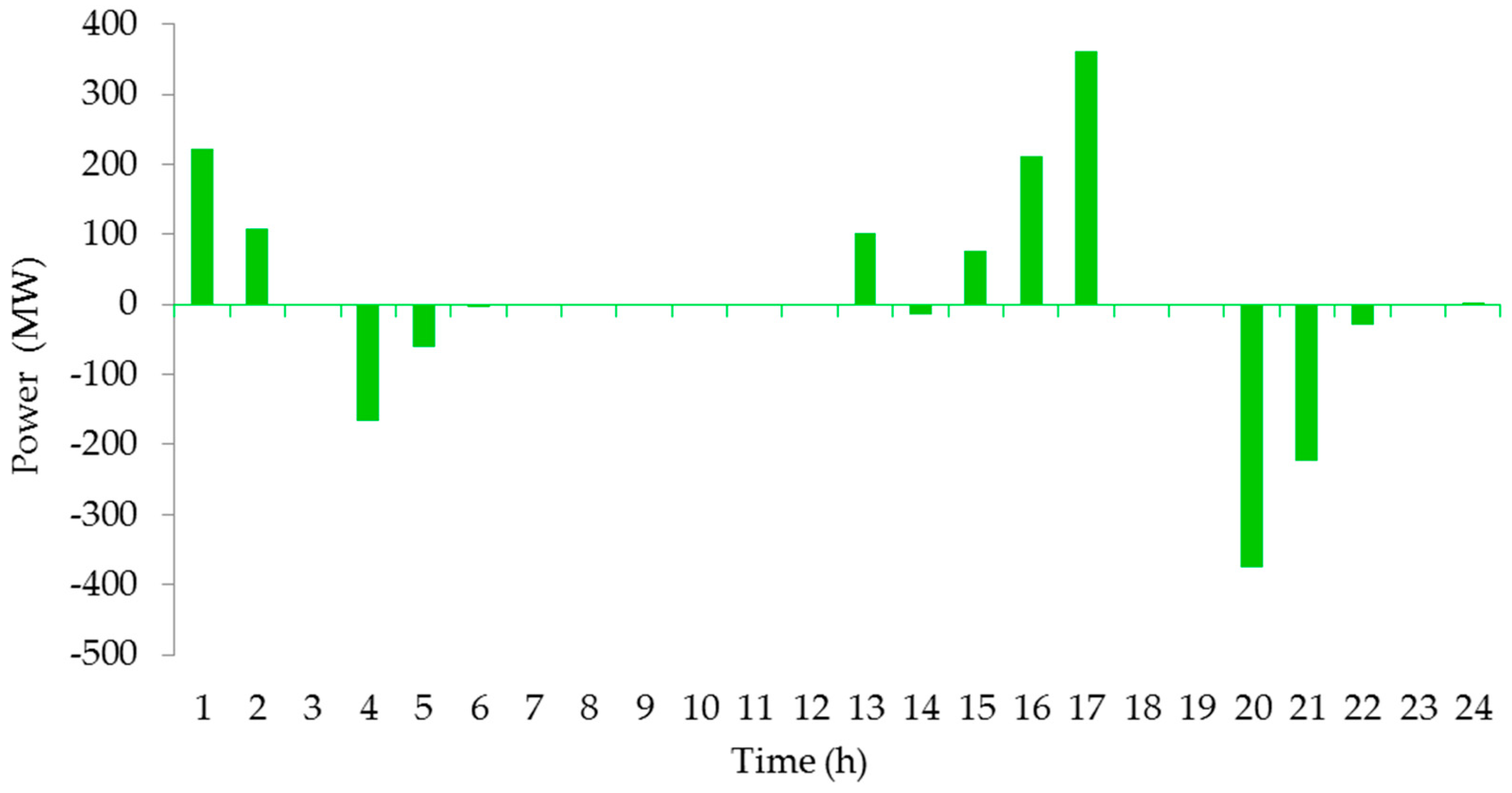
4.2.1. Results in Case 1

The power outputs of thermal generators in Case 1 are shown in Figure 12. The power outputs of pumped storage are shown in Figure 13, where the positive power means the operation state is as loads absorbing power from grid and the negative power means the operation state is generating power.

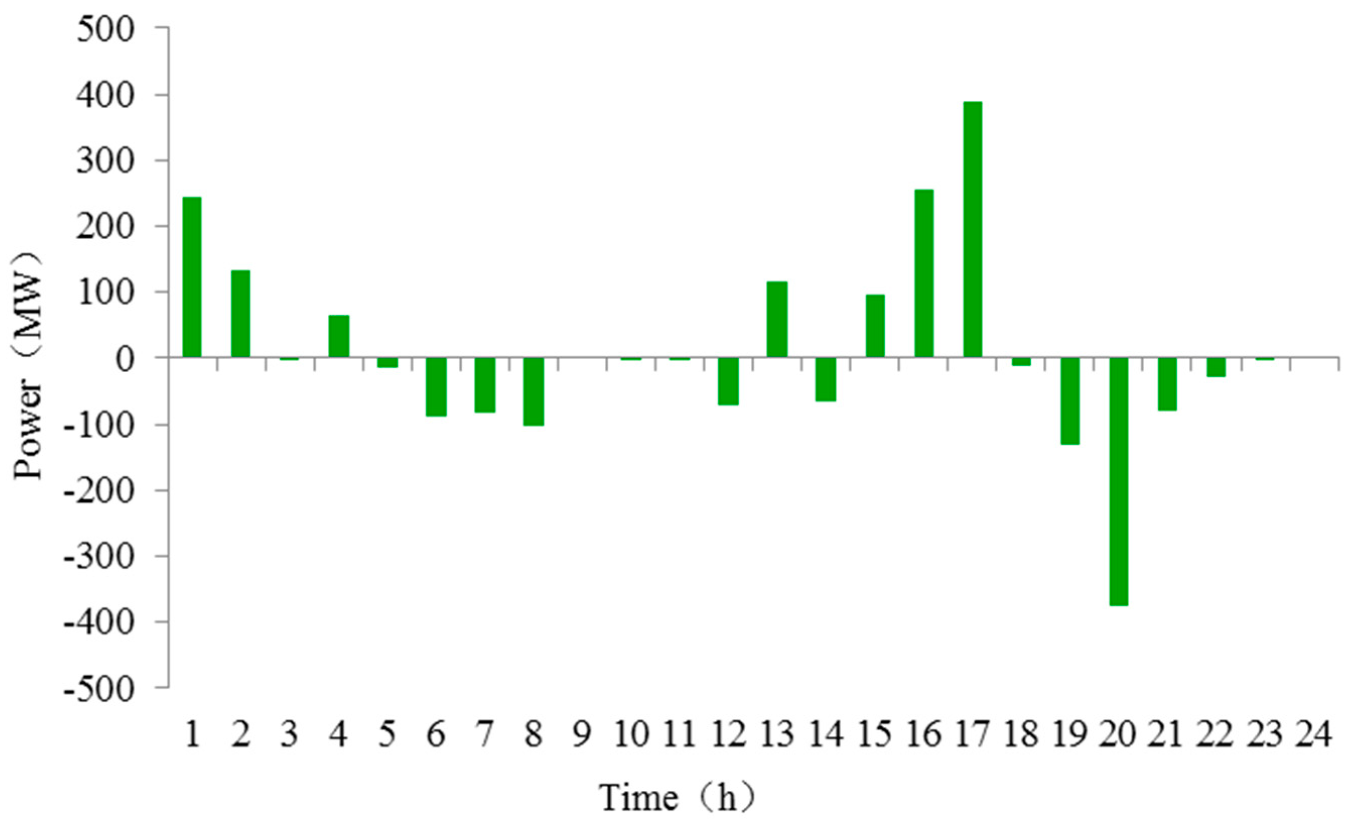
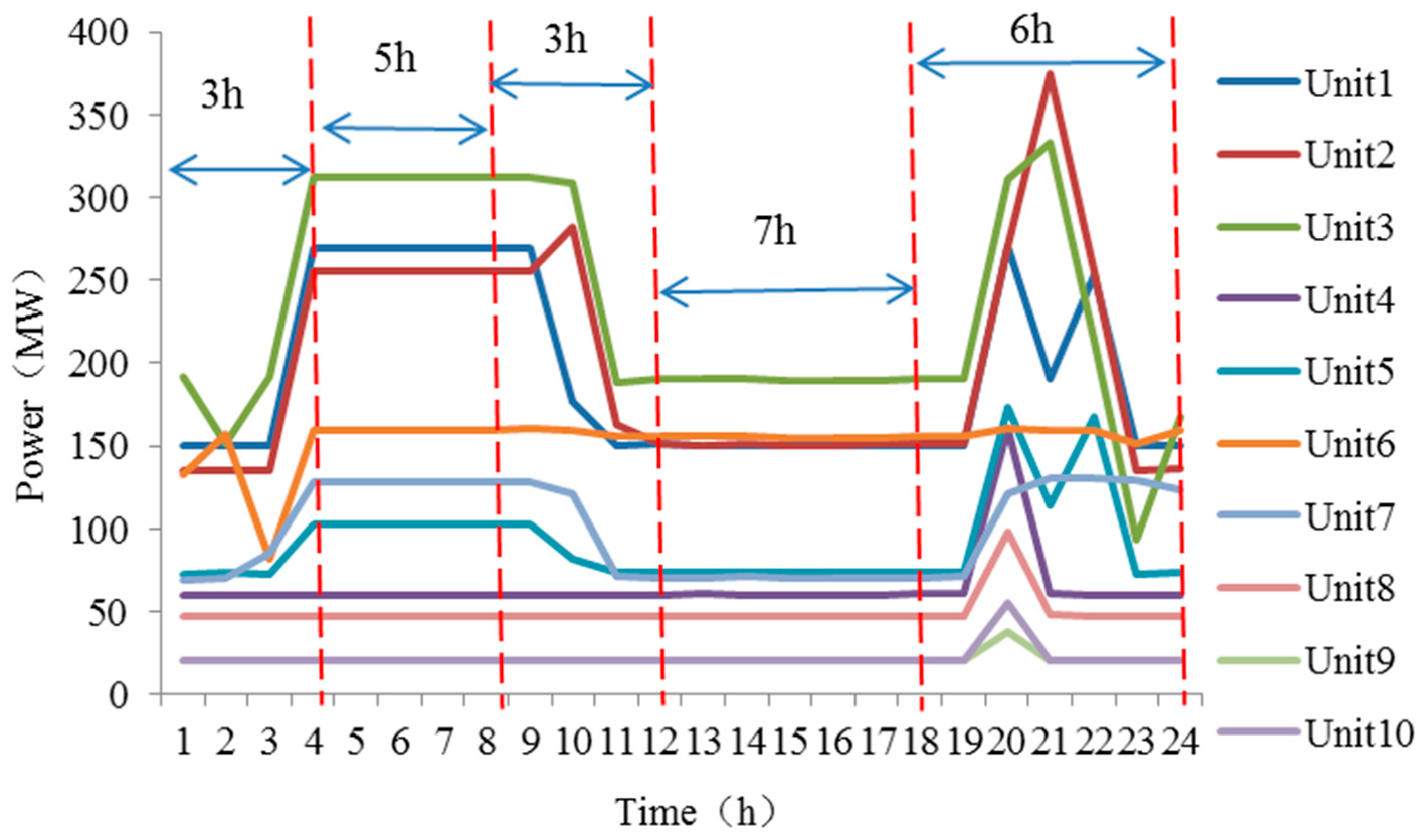
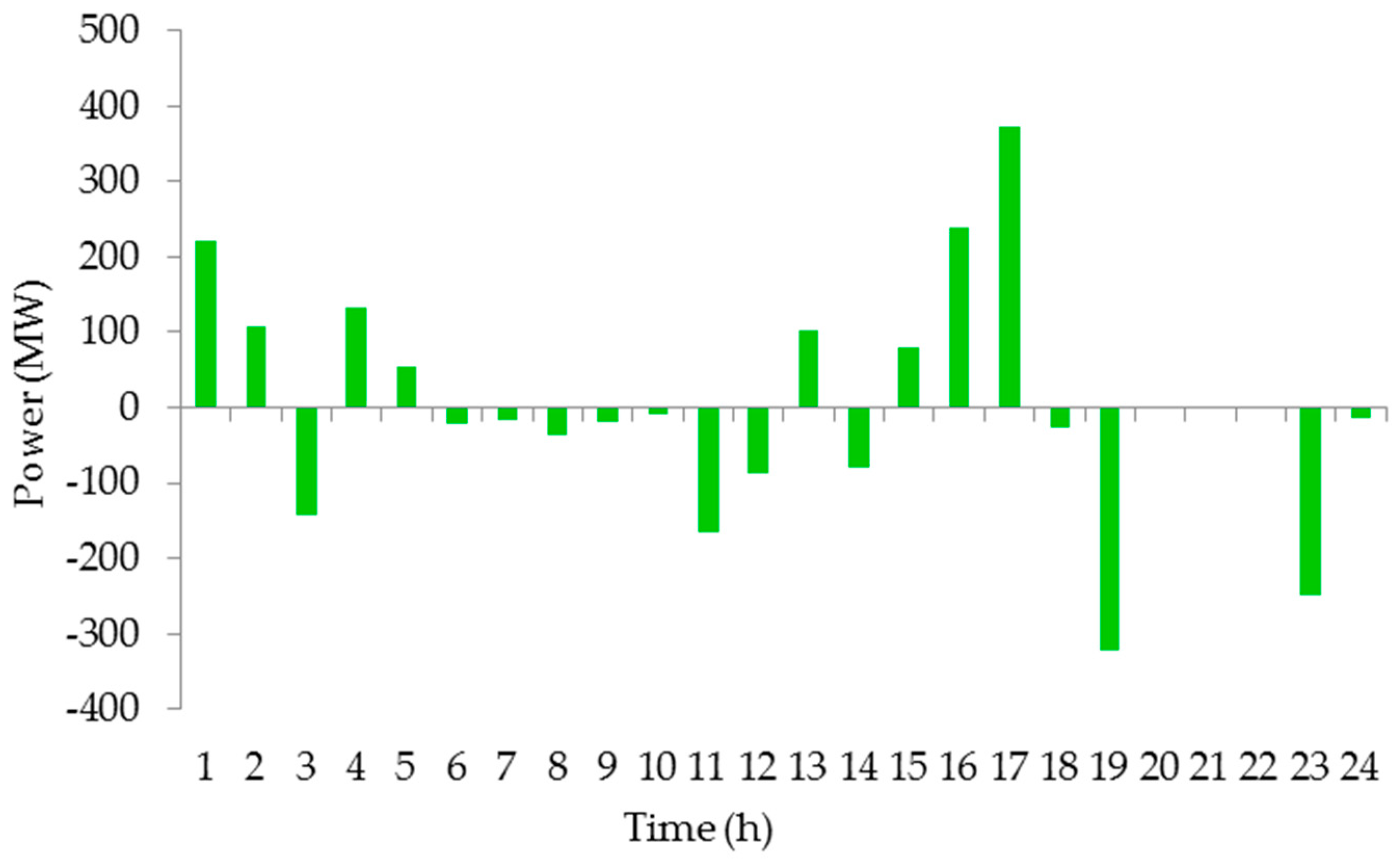
4.2.2. Results in Case 2

The power outputs of thermal generators based on the SampEn in Case 2 are shown in Figure 14. The power outputs of pumped storage are shown in Figure 15, where the positive power means the operation state is as loads absorbing power from grid and the negative power means the operation state is generating power. The power output comparisons of pumped storage in Case 1 and Case 2 are shown in Figure 16.

4.2.3. Results in Case 3

The power outputs of thermal generators in Case 3 are shown in Figure 17. The power outputs of pumped storage are shown in Figure 18, where the positive power means the operation state is as loads absorbing power from grid and the negative power means the operation state is generating power.

4.2.4. Results in Case 4

The power outputs of thermal generators based on the SampEn in Case 4 are shown in Figure 19. The power outputs of pumped storage are shown in Figure 20, where the positive power means the operation state is as loads absorbing power from grid and the negative power means the operation state is generating power. The power output comparisons of pumped storage in Case 3 and Case 4 are shown in Figure 21.

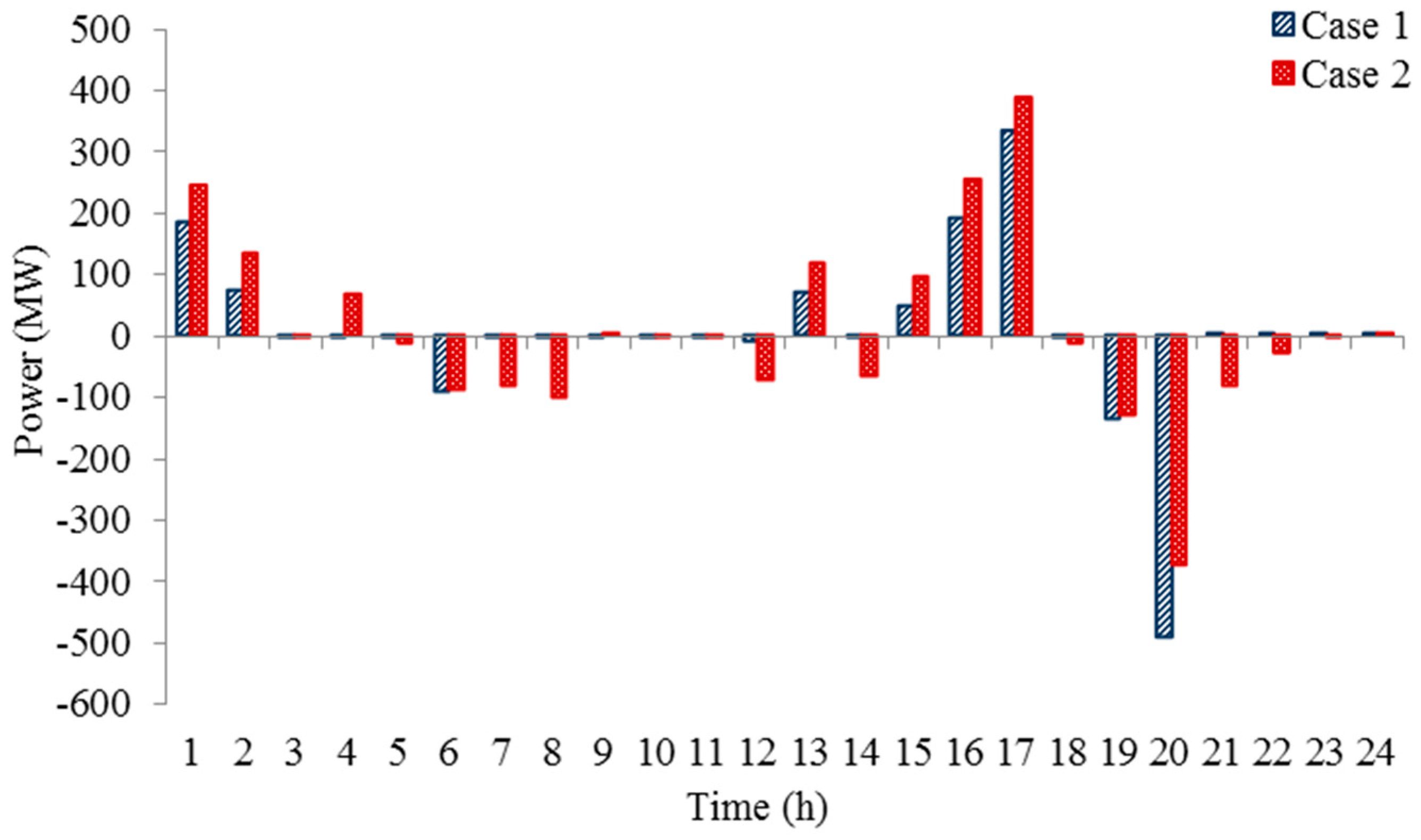
4.2.5. Result Comparison of Case 1 and Case 2

The operation costs, total up and down ramping power of thermal generators in Case 1 and Case 2 are shown in Table 4 together with the throughput power of pumped storage.

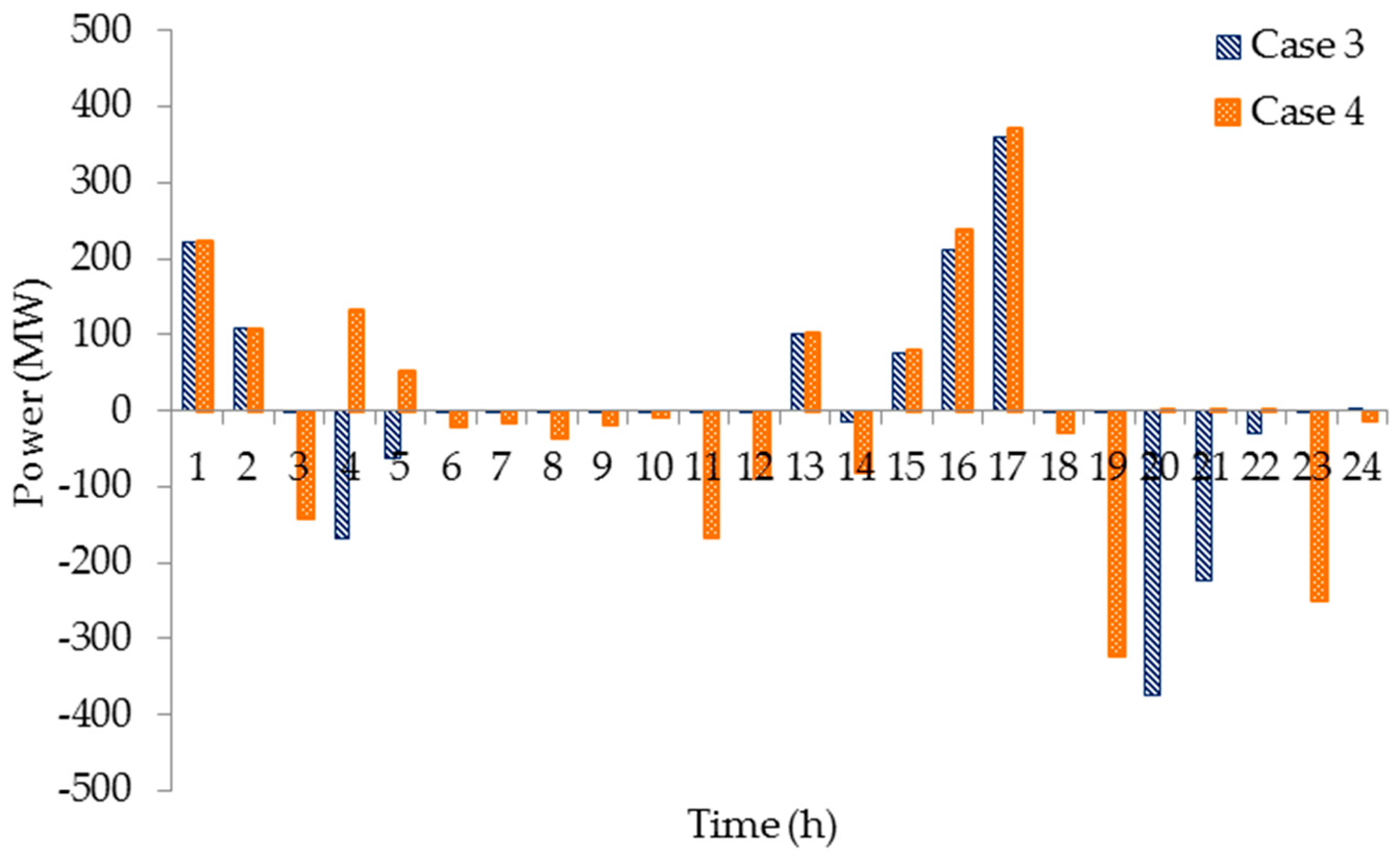
4.2.6. Result Comparison of Case 3 and Case 4

The operation costs, throughput power of pumped storage, total up and down ramping power of thermal generators in Case 3 and Case 4 are shown in Table 5.

4.3. Discussion

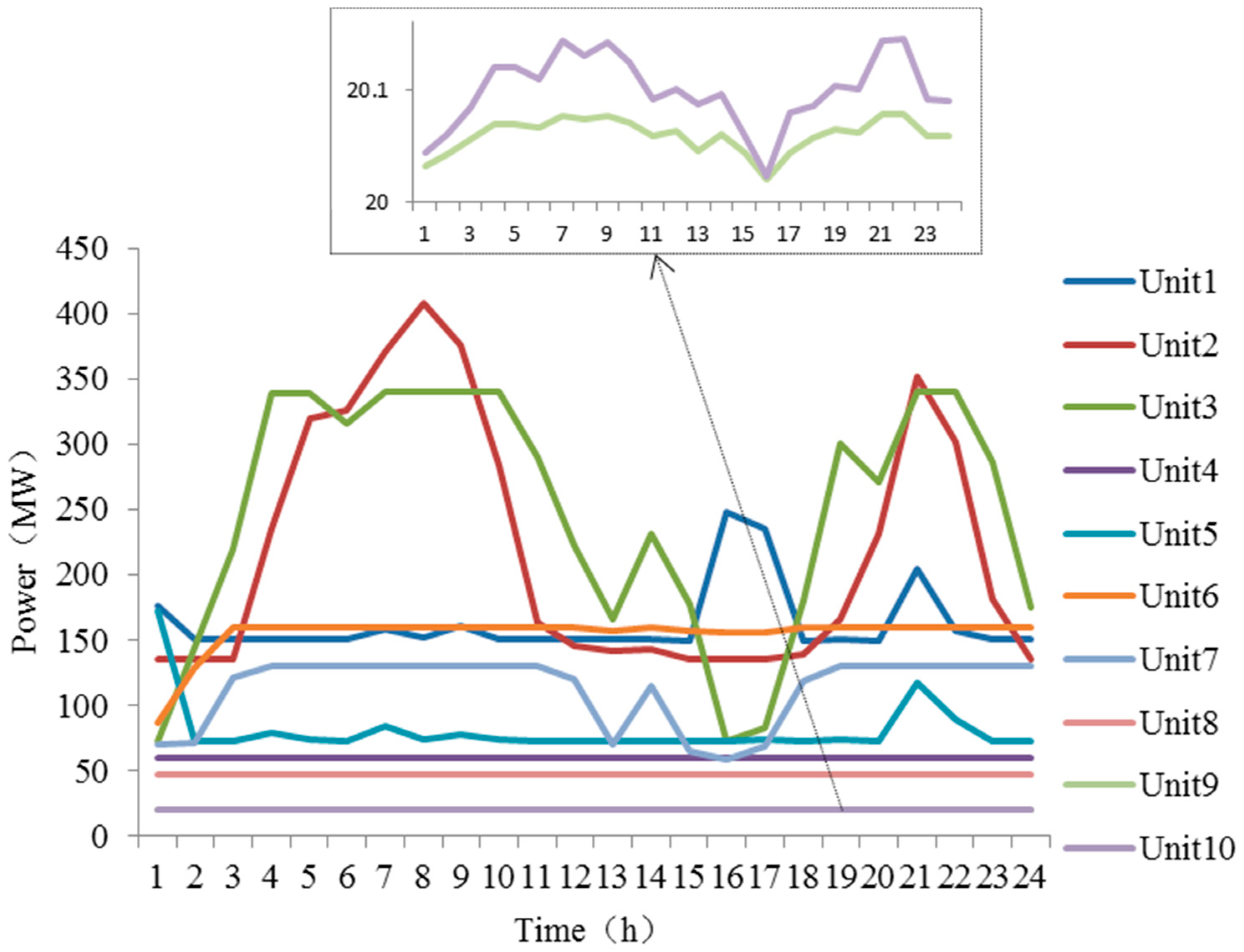
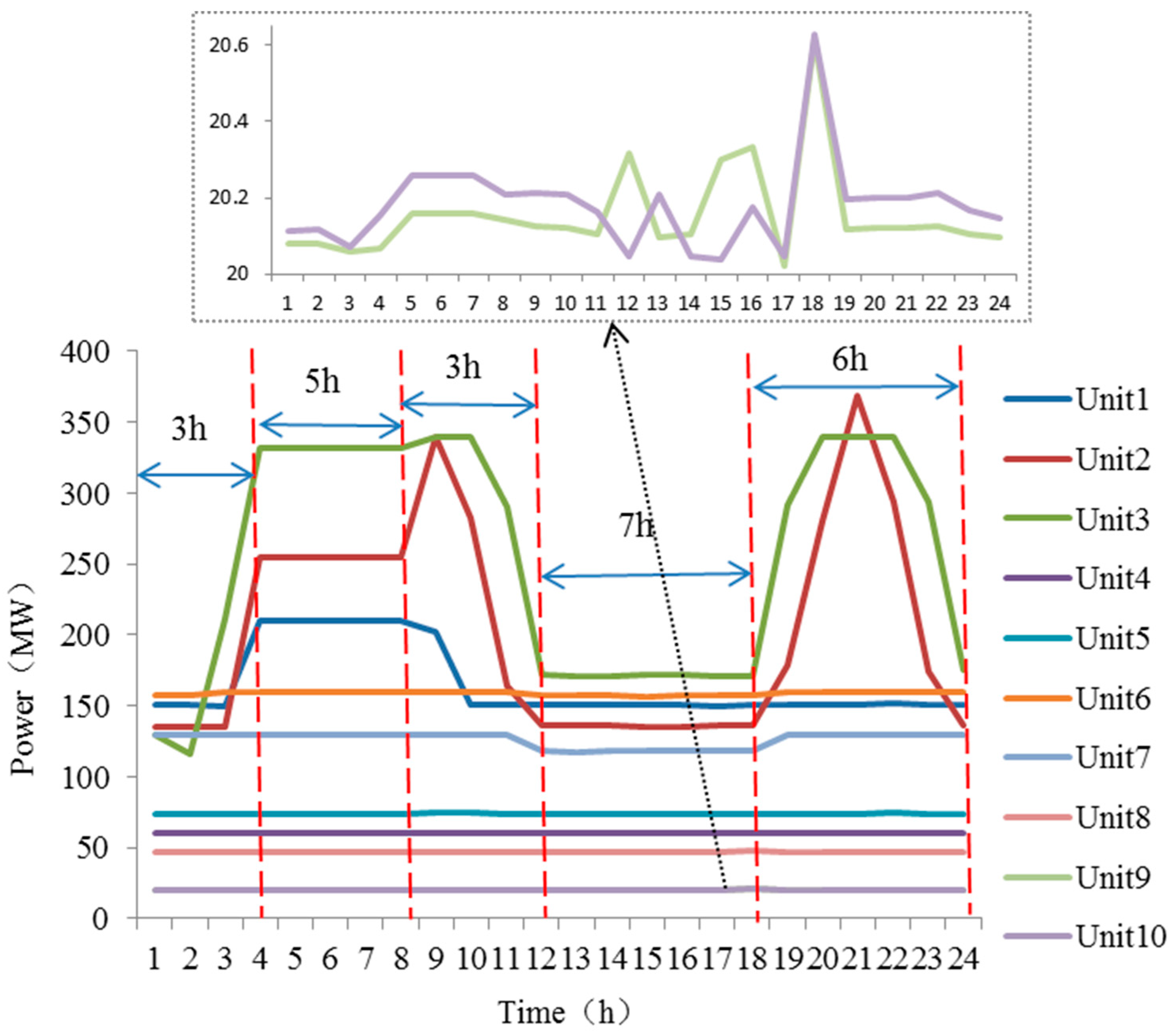
4.3.1. Power Outputs Analysis of Thermal Generators

The power output of thermal generators in Case 1–Case 4 are shown in Figure 12, Figure 14, Figure 17 and Figure 19, respectively. The power outputs of Unit 8 and Unit 9 are similar thus the power output curve of Unit 9 is covered by the one of Unit 8. The optimization in Case 1 and Case 3 aim at minimizing the operational costs. Apart from the traditional operation constraints, the power output plan also pursues the maximum economy and responses to the uncertainty of renewable power energies. Through the net load tracing and SampEn calculation, the power outputs are as Figure 14 and Figure 19 shows. For the time periods with high complexity level net loads, the power outputs of thermal generators are limited according to SampEn. For example, as Table 3 shows, in the second time period (duration is 5 h) and the fourth time period (duration is 7 h), the SampEn are large. The thermal generators are limited and forced to operate continuously and stability. Therefore, the operation is kept stable and the generator efficiency is increased together with the ramping power in these time periods reduced.
In the first, third, and fifth time periods, the SampEn is small, and there will be obviously power increase or decrease and last for hours. Thus, thermal generators need to respond to these power changes. Through the adjustment based on SampEn, the generating mode of thermal generators is settled as “3-5-3-7-6” in this simulation. Moreover, the time scales of the generating mode are corresponding to the results of SampEn.

4.3.2. Power Output Analysis of Pumped Storage

As shown in Figure 13 and Figure 18, at the initial period of time, in order to respond to the load increases in the second time period, the pumped storage in Case 1 and Case 3 should be activated and absorb power from power grid. The absorption of the pumped storage would store the redundant power from the grid for the net load peak time, during which the most amount of energies are required. Thus, the overall system efficiency is increased.
In Case 2 and Case 4 as shown in Figure 15 and Figure 20, at the initial period of time, the pumped storage absorbs power from power grid. However, the power outputs of thermal generators are kept stable or changes slightly. Thus, according to the Equations (6) and (7), the power is absorbed from the renewable energy in the net loads. As Figure 16 and Figure 21 show, during the time periods with high net load complexity level, the throughput of pumped storage is increased in Case 2 and Case 4. The power output adjustment of pumped storage response to the fluctuation of net loads instead of thermal generators. In addition, according to the generating mode of “3-5-3-7-6”, during the “5” and “7” time periods, the thermal power is kept stable and the changes of pumped storage take full response to the fluctuation of net loads. Thus, this strategy increases the interaction between pumped storage and renewable energies and stabilizes the thermal power, which further improves the stability of the system.

4.3.3. Power Output Analysis of the Cases with and Without SampEn

Table 4 shows that, the total operation cost of thermal generators in Case 2 is slightly less than that in Case 1. The result in Case 2 based on SampEn is only 0.04% less than in Case 1, but the operation status of thermal generators has been optimized. In Case 2, the total up and down ramping power have been both optimized up to around 43% compared to the results in Case 1. Moreover, the throughput of pumped storage in Case 2 is 44% more than that in Case 1. Table 5 shows that, the total operation cost of thermal generators in Case 4 is less than that in Case 3. The result in Case 4 based on SampEn is only 0.25% less than in Case 3, but the total up and down ramping power have been both optimized up to around 13% compared to the results in Case 3. Moreover, the throughput of pumped storage in Case 4 is 28% more than that in Case 3.
The overall results show that through the net load tracing and SampEn calculation, the original operation status with large fluctuation is transformed into the generating mode of “3-5-3-7-6”. Thus, the continuity and stability operation of thermal generators are realized and the operation efficiency of the system is improved. The power dispatch strategy based on SampEn can reduce the ramping power of thermal generators while ensuring both the economy and safety of the system.

5. Conclusions

This paper has presented a net load tracing dispatch strategy based on SampEn focusing on the high-percentage renewable energy connected to the power grid. A specific generating mode of thermal generators is determined by the net load tracing and SampEn. The conclusions based on the simulation results are as follows:
1. In the strategy, the renewable energies have priority to connect to power grid and the net loads are the dispatch objects. The renewable energies consumed by traditional loads totally and the curtailment of the wind and photovoltaic power are prevented. Thus, the utilization efficiency of renewable energies is maximized.
2. According to the net load tracing, the SampEn reflecting the complexity of net loads is calculated depending on the analysis of the characteristics and numeric features of net loads. Moreover, based on SampEn, the generating mode of thermal generators, the main power sources response to the fluctuation of renewable energies and their generating and ramping characteristics in different time periods are determined.
3. The interaction between pumped storage and renewable energies is increased in the dispatch based on SampEn. The pumped storage is responsible for the fluctuation of renewable energies instead of thermal generators in the certain time periods, during which the net loads are with large SampEn. Thus, the throughput of pumped storage is increased 44% in Case 2 and 27% in Case 4.
4. In this proposed strategy, the power outputs of thermal generators are smoothed and the generating time periods are optimized. The duration of stable operation of the thermal generators is increased and the ramping power during the time periods, in which the net loads are with large SampEn, are reduced 43% in Case 2 and 13% in Case 4. Overall, the stability of the system is improved with the economy of the system is ensured.

Author Contributions

Data curation, F.P.; Formal analysis, S.H. and C.D.; Methodology, S.H.; Project administration, W.Z.; Supervision, H.S.; Validation, Z.G. and W.Z.; Writing—Original draft, S.H.; Writing—Review and editing, H.S.

Funding

This research received no external funding.

Acknowledgments

This work is supported by The Science and Technology Project of State Grid (2017YF-20, 2017YF-27).

Conflicts of Interest

The authors declare no conflict of interest.

References

  1. Zhou, X.X.; Chen, S.Y.; Lu, Z.X.; Huang, Y.H.; Ma, S.C.; Zhao, Q. Technology features of the new generation power system in China. Proc. CSEE 2018, 38, 1893–1904. [Google Scholar]
  2. Krishnan, S.H.; Ezhilarasi, D.; Uma, G.; Umapathy, M. Pyroelectric-based solar and wind energy harvesting system. IEEE Trans. Sustain. Energy 2014, 5, 73–81. [Google Scholar] [CrossRef]
  3. Hsiao, C.C.; Jhang, J.W.; Siao, A.S. Study on pyroelectric harvesters integrating solar radiation with wind power. Energies 2015, 8, 7465–7477. [Google Scholar] [CrossRef]
  4. Xu, F.; Li, L.L.; Chen, Z.X.; Tu, M.F.; Ding, Q. Generation scheduling model and application with fluctuation reduction of unit output. Autom. Electr. Power Syst. 2012, 36, 45–50+102. [Google Scholar]
  5. Wood, A.J.; Wollenberag, B.F. Power Generation Operation and Control; Wiley: New York, NY, USA, 1996. [Google Scholar]
  6. Bai, J.H.; Xin, S.X.; Liu, J.; Zheng, K. Roadmap of realizing the high penetration renewable energy in China. Proc. CSEE 2015, 35, 3699–3705. [Google Scholar]
  7. Huber, M.; Dimkova, D.; Hamacher, T. Integration of wind and solar power in Europe: Assessment of flexibility requirements. Energy 2014, 69, 236–246. [Google Scholar] [CrossRef] [Green Version]
  8. Min, C.G.; Kim, M.K. Net load carrying capability of generating units in power systems. Energies 2017, 10, 1221. [Google Scholar] [CrossRef]
  9. Zhou, B.R.; Geng, G.C.; Jiang, Q.Y. Hydro-thermal-wind coordination in day-ahead unit commitment. IEEE Trans. Power Syst. 2016, 31, 4626–4637. [Google Scholar] [CrossRef]
  10. Jiang, R.; Wang, J.; Guan, Y. Robust unit commitment with wind power and pumped storage hydro. IEEE Trans. Power Syst. 2012, 27, 800–810. [Google Scholar] [CrossRef]
  11. Hu, S.B.; Sun, H.; Peng, F.X.; Zhou, W.; Cao, W.P.; Su, A.L.; Chen, X.D.; Sun, M.Z. Optimization strategy for economic power dispatch utilizing retired EV batteries as flexible loads. Energies 2018, 11, 1657. [Google Scholar] [CrossRef]
  12. Ortega-Vazquez, M.A.; Kirschen, D.S. Estimating the spinning reserve requirements in systems with significant wind power generation penetration. IEEE Trans. Power Syst. 2009, 24, 114–124. [Google Scholar] [CrossRef]
  13. Papavasiliou, A.; Oren, S.S.; O’Neill, R.P. Reserve requirements for wind power integration: A scenario-based stochastic programming framework. IEEE Trans. Power Syst. 2011, 26, 2197–2206. [Google Scholar] [CrossRef]
  14. Matos, M.A.; Bessa, R.J. Setting the operating reserve using probabilistic wind power forecasts. IEEE Trans. Power Syst. 2011, 26, 594–603. [Google Scholar] [CrossRef]
  15. Lannoye, E.; Flynn, D.; O’Malley, M. Assessment of power system flexibility: A high-level approach. In Proceedings of the IEEE Power & Energy Society General Meeting, San Diego, CA, USA, 22–26 July 2012; pp. 1–8. [Google Scholar]
  16. Wu, Y.K.; Chang, L.T.; Su, P.E.; Hsieh, T.Y.; Jan, B.S. Assessment of potential variability of net load following the integration of 3 GW wind power in Taiwan. Energy Procedia 2016, 100, 117–121. [Google Scholar] [CrossRef]
  17. Marannino, P.; Granelli, G.P.; Montagna, M.; Silvestri, A. Different time-scale approaches to the real power dispatch of thermal units. IEEE Trans. Power Syst. 1990, 5, 169–176. [Google Scholar] [CrossRef]
  18. Generation Dispatching Plan of Electricity Market on Generation Side. Available online: http://tech.bjx.com.cn/html/20071227/59347.shtml (accessed on 25 December 2018).
  19. Cataliotti, A.; Cervellera, C.; Cosentino, V.; Di Cara, D.; Gaggero, M.; Maccio, D.; Marsala, G.; Ragusa, A.; Tine, G. An Improved Load Flow Method for MV Networks Based on LV Load Measurements and Estimations. IEEE Trans. Instrum. Meas. 2018, 68, 430–438. [Google Scholar] [CrossRef]
  20. Cataliotti, A.; Cosentino, V.; Di Cara, D.; Tinè, G. LV Measurement Device Placement for Load Flow Analysis in MV Smart Grids. IEEE Trans. Instrum. Meas. 2016, 65, 999–1006. [Google Scholar] [CrossRef]
  21. Xygkis, T.C.; Korres, G.N. Optimized measurement allocation for power distribution systems using mixed integer sdp. IEEE Trans. Instrum. Meas. 2017, 66, 2967–2976. [Google Scholar] [CrossRef]
  22. Xygkis, T.C.; Korres, G.N.; Manousakis, N.M. Fisher information based meter placement in distribution grids via the d-optimal experimental design. IEEE Trans. Smart Grid 2018, 9, 1452–1461. [Google Scholar] [CrossRef]
  23. Pegoraro, P.A.; Angioni, A.; Pau, M.; Monti, A.; Muscas, C.; Ponci, F.; Sulis, S. Bayesian approach for distribution system state estimation with non-gaussian uncertainty models. IEEE Trans. Instrum. Meas. 2017, 66, 2957–2966. [Google Scholar] [CrossRef]
  24. Zhang, L.; Yang, J.; Jian, X.H.; Zhang, F.; Han, X.S. Unit Commitment with Energy Storage Considering Operation Flexibility at Sub-hourly Time-scales. Autom. Electr. Power Syst. 2018, 42, 48–56. [Google Scholar]
  25. Zhai, J.Y.; Ren, J.W.; Zhou, M.; Li, Z. Multi-Time Scale Fuzzy Chance Constrained Dynamic Economic Dispatch Model for Power System with Wind Power. Power Syst. Technol. 2016, 40, 1094–1099. [Google Scholar]
  26. Yong, T.; Yao, J.; Yang, S.; Yang, Z. Ramp enhanced unit commitment for energy scheduling with high penetration of renewable generation. In Proceedings of the 2015 IEEE Power & Energy Society General Meeting, Denver, CO, USA, 26–30 July 2015. [Google Scholar]
  27. Zhao, D.M.; Yin, J.F. Fuzzy random chance constrained preemptive goal programming scheduling model considering source-side and load-side uncertainty. Trans. China Electrotech. Soc. 2018, 33, 1076–1085. [Google Scholar]
  28. Li, P.; Wand, X.Y.; Han, P.F. Risk Analysis of Microgrid Optimal Operation Scheduling under Double Uncertainty Environment. Proc. CSEE 2017, 37, 4296–4303. [Google Scholar]
  29. Guo, P.; Wen, J.; Zhu, D.D.; Wang, W.Z.; Liu, W.Y. The Coordination Control Strategy for Large-Scale Wind Power Consumption Based on Source-Load Interactive. Trans. China Electrotech. Soci. 2017, 32, 1–9. [Google Scholar]
  30. Zhang, X.H.; Zhao, C.M.; Liang, J.X.; Li, K.; Zhong, J.Q. Robust Fuzzy Scheduling of Power Systems Considering Bilateral Uncertainties of Generation and Demand Side. Autom. Electr. Power Syst. 2018, 42, 67–75. [Google Scholar]
  31. Gangammanavar, H.; Sen, S.; Zavala, V.M. Stochastic optimization of sub-hourly economic dispatch with wind energy. IEEE Trans. Power Syst. 2016, 31, 949–959. [Google Scholar] [CrossRef]
  32. Wang, J.D.; Wang, J.H.; Liu, C.; Ruiz, J.P. Stochastic unit commitment with sub-hourly dispatch constraints. Appl. Energy 2013, 105, 418–422. [Google Scholar] [CrossRef]
  33. Zhang, X.Y.; Yang, J.Q.; Zhang, X.J. Dynamic economic dispatch incorporating multiple wind farms based on FFT simplified chance constrained programming. J. Zhengjiang Univ. (Eng. Sci.) 2017, 51, 976–983. [Google Scholar]
  34. Shaker, H.; Zareipour, H.; Wood, D. Impacts of large-scale wind and solar power integration on California’s net electrical load. Renew. Sustain. Energy Rev. 2016, 58, 761–774. [Google Scholar] [CrossRef]
  35. Yin, Y.; Shang, P.J.; Andrew, C.A.; Peng, C.K. Multiscale joint permutation entropy for complex time series. Physica A 2019, 515, 388–402. [Google Scholar] [CrossRef]
  36. Cuadras, A.; Romero, R.; Ovejas, V.J. Entropy characterisation of overstressed capacitors for lifetime prediction. J. Power Sources 2016, 336, 272–278. [Google Scholar] [CrossRef]
  37. Hsiao, C.C.; Liang, B.H. The generated entropy monitored by pyroelectric sensors. Sensors 2018, 18, 3320. [Google Scholar] [CrossRef] [PubMed]
  38. Zhang, Y.Y. The Theory of Approximate Entropy and its Application. Chin. J. Med. Phys. 2009, 26, 1543–1546. [Google Scholar]
  39. Chou, C.M. Complexity analysis of rainfall and runoff time series based on sample entropy in different temporal scales. Stoch. Environ. Res. Risk Assess. 2014, 28, 1401–1408. [Google Scholar] [CrossRef]
  40. Richman, J.S.; Moorman, J.R. Physiological time-series analysis using approximate entropy and sample entropy. Am. J. Physiol. Heart Circ. Physiol. 2000, 278, 2039–2049. [Google Scholar] [CrossRef] [PubMed]
  41. Zhang, Y.C.; Liu, K.P.; Qin, L.; Fang, N.C. Wind Power Multi-Step Interval Prediction Based on Ensemble Empirical Mode Decomposition-Sample Entropy and Optimized Extreme Learning Machine. Power Syst. Technol. 2016, 40, 2045–2051. [Google Scholar]
  42. Al-Angari, H.M.; Sahakian, A.V. Use of sample entropy approach to study heart rate variability in obstructive sleep apnea syndrome. IEEE Trans. Bio-Med. Eng. 2007, 54, 1900–1904. [Google Scholar] [CrossRef]
  43. Xu, W. The Complexity Algorithms Research of Chaotic Sequences Based on Entropy Theory. Ph.D. Thesis, Heilongjiang University, Harbin, China, 2017. [Google Scholar]
  44. Zhang, X.Q.; Liang, J.; Zhang, X.; Zhang, F.; Zhang, L.; Xu, B. Combined Model for Ultra Short-term Wind Power Prediction Based on Sample Entropy and Extreme Learning Machine. Proc. CSEE 2013, 33, 33–40. [Google Scholar]
  45. Cheng, W.S.; Zhang, H.F. A dynamic economic dispatch model incorporating wind power based on chance constrained programming. Energies 2015, 8, 233–256. [Google Scholar] [CrossRef]
  46. Shen, Z.; Xie, S.Q.; Pan, C.Y. Probability and Statistics; High Education Press: Beijing, China, June 2008; pp. 139–143, 161–163. [Google Scholar]
  47. Attaviriyanupap, P.; Kita, H.; Tanaka, E.; Hasegawa, J. A hybrid EP and SQP for dynamic economic dispatch with nonsmooth fuel cost function. IEEE Trans. Power Syst. 2002, 17, 411–416. [Google Scholar] [CrossRef]
  48. Zhang, X.H.; Zhao, J.Q.; Chen, X.Y. Multi-objective Unit Commitment Fuzzy Modeling and Optimization for Energy-saving and Emission Reduction. Proc. CSEE 2010, 30, 71–76. [Google Scholar]
Figure 1. Actual load curve of one province from 3 March to 24 April.
Energies 12 00193 g001
Figure 2. Actual wind power curve of one province from 3 March to 24 April.
Energies 12 00193 g002
Figure 3. Net load curve of one province from 3 March to 24 April.
Energies 12 00193 g003
Figure 4. Net load curve and the adjacent point slope of 11 April, (a) The consecutive point slope; (b) The net load curve.
Energies 12 00193 g004
Figure 5. Net load curve and the adjacent point slope of 3 March, (a) The consecutive point slope; (b) The net load curve.
Energies 12 00193 g005aEnergies 12 00193 g005b
Figure 6. Beta distribution curve.
Energies 12 00193 g006
Figure 7. Flow chart of power system net load tracing dispatch based on sample entropy.
Energies 12 00193 g007
Figure 8. Load curve.
Energies 12 00193 g008
Figure 9. Prediction wind power curve and the power output limit curve of different confidence degrees.
Energies 12 00193 g009
Figure 10. Photovoltaic power output curve.
Energies 12 00193 g010
Figure 11. Net load curve.
Energies 12 00193 g011
Figure 12. Power output curves of thermal generators in Case 1.
Energies 12 00193 g012
Figure 13. Power output curves of pumped storage generators in Case 1.
Energies 12 00193 g013
Figure 14. Power output curves of thermal generators in Case 2.
Energies 12 00193 g014
Figure 15. Power output curves of pumped storage in Case 2.
Energies 12 00193 g015
Figure 16. Power output comparisons of pumped storage in Case 1 and Case 2.
Energies 12 00193 g016
Figure 17. Power output curves of thermal generators in Case 3.
Energies 12 00193 g017
Figure 18. Power output curves of pumped storage generators in Case 3.
Energies 12 00193 g018
Figure 19. Power output curves of thermal generators in Case 4.
Energies 12 00193 g019
Figure 20. Power output curves of pumped storage in Case 4.
Energies 12 00193 g020
Figure 21. Power output comparisons of pumped storage in Case 3 and Case 4.
Energies 12 00193 g021
Table 1. Data for the net load of a province on 3 March and 4 April
DateTimeSlope Sign Changing AmountPercentage of Slope Sign ChangingValley-to-PeakSlope Sign Changing Amount/Valley-to-PeakSampEn
04111–18110.61731.610.01500.42
19–4130.13457.950.00660.18
42–69150.54247.650.06060.74
70–9610.04795.910.00130.08
03031–4560.132582.030.00230.04
46–96180.35340.370.05290.72
Table 2. Operating data for the 10-unit system
ParametersUnit1Unit2Unit3Unit4Unit5Unit6Unit7Unit8Unit9Unit10
P max (MW)4704603403002431601301208055
P min (MW)1501357360735720472020
a (10−3 $/MW2h)0.430.630.390.700.790.562.114.80109.089.51
B ($/MWh)21.6021.0520.8123.9021.6217.8716.5123.2319.5822.54
C ($/h)958.201313.6604.97471.60480.29601.75502.70639.40455.60692.40
UR12012012010010010050505050
DR12012012010010010050505050
C o e U R i ($/MWh)14.715.515.217.819.319.818.721.723.425.2
C o e D R i ($/MWh)15.214.815.118.621.219.5192223.125.6
C o e r a m p u p i ($/MWh)3.133.083.754.175.889.719.0913.716.6728.57
C o e r a m p d o w n i ($/MWh)3.133.083.754.175.889.719.0913.716.6728.57
Table 3. Data for the SampEn of net load
Time Periods (h)SampEnSampEn Proportion
1–40.045%
4–80.1416%
8–120.082%
12–180.6171%
18–240.066%
Table 4. Results comparison of Case 1 and Case 2
ParametersCase 1Case 2Percentage Optimization of Case 2 Compared to Case 1
Operation cost (105 $)7.17447.17120.04%
Up ramping power (MW)1636.27918.5943.86%
Down ramping power (MW)1526.61869.3743.05%
Throughput of pumped storage (MW)1636.032358.2944.15%
Table 5. Results comparison of Case 3 and Case 4
ParametersCase 3Case 4Percentage Optimization of Case 4 Compared to Case 3
Operation cost (105 $)7.20827.19030.25%
Up ramping power (MW)1932.881681.8912.99%
Down ramping power (MW)1860.821623.4712.76%
Throughput of pumped storage (MW)1955.612497.8227.73%

