1. Introduction
In the modern era, there is an increasing need for modelling financial markets (and engineering sciences, e.g., signal detection) with high volatility. An important characteristic of such a probability distribution is its tail behaviour, determined through its tail thickness. There is a need for modelling such financial data. High variability has also been a common characteristic of modern circular data.
Corresponding circular distributions are characterised by heavy or long tails. The normal and Cauchy distributions, and, sometimes, a mixture of the normal and Cauchy distributions, are suitable for modelling such financial data. The family of stable distributions can provide better modelling for such financial data sets. Highly volatile financial time-series data may be better modelled, in many cases, by the Linnik distribution in comparison to the stable distribution, e.g., see
Anderson and Arnold (
1993). This highly flexible family of distributions is better capable of modelling the inflection points and tail behaviour compared to the existing popular flexible symmetric unimodal models.
There have been a lot of studies establishing the use of the Linnik family of distributions as a highly flexible, important, and useful family for modelling financial data. However, its implementation for real-life data seems to have been somewhat restricted, possibly because of the lack of a simple and efficient estimator of the parameter, particularly that of the index parameter . The estimation of the tail thickness of heavy-tailed financial data using the index parameter is important in the context of modelling.
Our aim in this paper is to provide a universal (for all ), efficient, and easily implementable estimator of after presenting a review of the few existing methods. The issue behind the derivation is to study the advantages and also to point out the shortcomings of some of the estimators and hence to obtain better estimators that eliminate the effects of the shortcomings of the former ones.
We have observed that the circular-statistics-based estimators can be quite useful in this context, which is enhanced in this paper. Circular statistics are obtained for circular data. In many emerging real-life situations, we not only make observations on linear variables but also on circular ones, that is, on angular propagations, orientations, directional movements, and strictly periodic occurrences. Such data are referred to as directional data, which, in two dimensions, are known as circular data. Linear data may be transformed into circular data using the method of wrapping.
Here, we recall two highly flexible families of circular distributions, e.g., the wrapped stable family, in
Section 2, and the wrapped Linnik family in
Section 3, and the novel, universal, efficient, and easily implementable estimators of
derived from these are presented in
Section 7. In
Section 4, descriptions of the classical Hill estimator by
Hill (
1975), and its generalisation by
Brilhante et al. (
2013), are presented. In
Section 5, the fractional moment estimator for the symmetric Linnik distribution proposed by
Kozubowski (
2001) is reviewed. The fractional moment estimator of the characteristic exponent used to measure the tail thickness for skewed stable distributions, proposed by
Kuruoglu (
2001), is particularised to obtain the same for the symmetric stable distribution in
Section 5. In
Section 6, the characteristic function-based estimator proposed by
Anderson and Arnold (
1993) is presented. In
Section 7, the trigonometric method of moment estimators proposed by
SenGupta (
1996) and
SenGupta and Roy (
2023) is presented, which is further modified to obtain an improved estimator (as in
SenGupta and Roy 2019,
2023) in
Section 8. The trigonometric method of moment estimation is exploited here for symmetric circular distributions only. It can be used for asymmetric distributions as well. But the computations involved are complicated and time consuming and hence are not considered here. In
Section 9, the performance of the estimators is discussed through extensive simulations, focusing on their estimated mean bias and estimated root-mean-square errors, as presented in
Table 1 and
Table 2. In
Section 10, the computed values of the estimators are obtained for two real-life financial data sets, which are presented in
Table 3. In
Section 11, novel tests for the index parameter
of the stable and Linnik distributions are introduced and also illustrated with real-life financial data. Some discussions and conclusions on the different estimators are provided in
Section 12. In the Acknowledgement section, the authors express their acknowledgements.
3. The Symmetric Linnik and the Wrapped Linnik Family of Distributions
It was established by
Pakes (
1998) that the characteristic function of a symmetric (
) Linnik (linear) distribution is given by
The density function cannot be written in an analytical form except for = 2. The wrapping of this distribution yields the wrapped symmetric Linnik family of distributions. However, this circular family differs from that of the symmetric wrapped stable family and none of these families is a sub-family of the other. In particular, taking for the wrapped symmetric stable family one gets the wrapped Cauchy, while for the wrapped symmetric Linnik family it gives the wrapped Laplace (double exponential) distribution.
Theorem 2. (a) The trigonometric moment of order p for a wrapped Linnik distribution corresponds to the value of the characteristic function of the linear Linnik random variable at the integer value p. (b) The characteristic function of the wrapped Linnik random variable θ at the integer p is The probability density function of wrapped Linnik distribution is defined as
where the parameter space is given by
We observe that these wrapped distributions preserve the parameter for the corresponding linear distributions.
Without a loss of generality, we take and in the following. The index parameter of the circular family of distributions plays an important role in determining the thickness and hence the tail behaviour of the distribution. There are, in fact, four possible names for the parameter . Some interpret it as the tail thickness parameter or the index parameter used to measure tail thickness mainly for heavy tailed distributions. Others interpret it as the characteristic exponent when it is present in an exponential form in a characteristic function. Sometimes, is also defined as the shape parameter along with its three other companions viz. location parameter , scale parameter , and skewness parameter . For this paper, we assume the symmetric case that is . Several estimators of this parameter have been developed over time.
4. Hill Estimator and Its Generalisation
The classical Hill estimator (see
Hill 1975;
Dufour and Kurz-Kim 2010), is a simple non-parametric estimator based on order statistics. Given a sample of
n observations
the Hill estimator is defined as
with standard error
where
k is the number of observations which lie on the tails of the distribution of interest and is to be optimally chosen depending on the sample size,
n, and tail thickness
, as
and
denotes the
j-order statistic of the sample of size
n.
The asymptotic normality of the classical Hill estimator is provided by
Goldie and Smith (
1987) as
which leads to the following lemma
This estimator uses the linear function of the order statistics and can be used to estimate only. Further, it is also “extremely sensitive” to the choice of the optimal number of tail observations k, which itself is a function of the unknown index parameter being estimated.
The Hill estimator is scale invariant since it is defined in terms of the log of ratios but not location invariant. Therefore, centering needs to be performed in order to address the location invariance.
The classical Hill estimator is actually the logarithm of the geometric mean or the logarithm of the mean of order
of a set of statistics. This estimator has been generalized to a more general mean of order
of the same set of statistics by
Brilhante et al. (
2013) as follows:
where the class of statistics
is taken as the mean of order
p of the statistics
given by
where
is the generalized inverse function of the cumulative distribution function
F of
X and using the distributional identity
with
Y as a unit Pareto random variable and
Under the first order condition that the generalized inverse function
is of regular variation with index
, the consistency of the generalized class of Hill estimators
is established, provided
. In addition, under the assumption of the second order condition, the asymptotic normality of
can also be obtained (see
Brilhante et al. 2013) as
holds for all
and
is asymptotically standard normal and
with
being the second-order parameter, controlling the rate of convergence for the first order condition.
5. Fractional Moment Estimator
Another alternative estimator of the index parameter
is given by
Kozubowski (
2001) as the usual method of moment estimator with fractional order. If
are realizations from the symmetric Linnik distribution with index parameter
and scale parameter
, then the
pth absolute moment is
where
and
. As suggested in
Kozubowski (
2001), using suitable choices of
p as
and 1 and solving the respective equations, the fractional moment estimator of the the index parameter
can be obtained. This estimator is valid only for
. To overcome this restriction, a universal and efficient estimator for both stable and Linnik distributions will appear in our next works.
If
are realizations from the symmetric stable distribution with index parameter
, scale parameter
, and location parameter 0, then the
pth absolute moment given by
Kuruoglu (
2001) is
where
,
and
. Using the method of moments with the corresponding sample moment,
and applying the following property of gamma function,
the fractional moment estimator of the index parameter
can be obtained.
7. The Trigonometric Moment Estimator
It is known, in general, by
Jammalamadaka and SenGupta (
2001) that the characteristic function of
at the integer
p is defined as,
Further by,
Jammalamadaka and SenGupta (
2001) we know that, for the p.d.f given by (
3),
Suppose
are a random sample of size
m drawn from the wrapped stable density given by (
3). We define
Then, we note that
and
.
Using the method of trigonometric moments estimation, and equating
and
to the corresponding functions of the theoretical trigonometric moments, we get the estimator of the index parameter
of wrapped stable distribution (see
SenGupta 1996):
Now, suppose
are a random sample of size
m drawn from the wrapped Linnik density given by (
5). Using the method of trigonometric moments estimation, and equating the empirical trigonometric moments
and
to the corresponding theoretical moments, we get the estimator of index parameter
of wrapped Linnik distribution (as obtained for the wrapped stable distribution by
SenGupta 1996),
where
,
and
is the mean direction given by
. Note that
.
The asymptotic normality of the estimators
and
have been established in the following Theorems 3 and 4 respectively (see
SenGupta and Roy 2019,
2023).
Theorem 4. , where
and Where m denotes the sample size and denotes the dispersion matrix of in both the above theorems.
Unlike for the previous estimators where at the most simulation results were given for the properties of the estimators, the asymptotic distributions obtained in the Theorems 3 and 4 establish rigorously the theoretical and the analytical properties of the trigonometric moment estimators. The estimators can be shown to be consistent and asymptotically normal(CAN) through the use of the theorems. Additionally, the usefulness of the theorems is to provide a methodology to rigorously test for the index parameter
which is illustrated in
Section 11.
8. The Truncated Trigonometric Moment Estimator
The moment estimators
and
need not always remain in the support of the true parameter
(that is (0,2]). Hence, the moment estimators proposed above need not be proper estimators of
. Hence, the modified estimators for wrapped stable and wrapped Linnik distribution free from this defect are, respectively, given by
and
(since the support of
excludes non-positive values).
The asymptotic normality of the modified truncated estimators
and
are established, respectively, in the following theorems (see
SenGupta and Roy 2019,
2023). We have
Theorem 5. where
where
where = and =
Theorem 6. where
where
where = and =
In both the above theorems, and denote the p.d.f and c.d.f of a standard normal variable respectively.
9. Efficiency of the Estimators
It is naturally of interest to see how close these estimators are. Here, we briefly discuss this aspect with an empirical sample. The raw financial data can be transformed into circular data by using the method of wrapping (see, e.g., page 31 of
Jammalamadaka and SenGupta (
2001)). That is, for positive (linear) values, after dividing by 2
, we take the remainder, while for negative (linear) values, we add 2
to the remainder to produce the corresponding circular values in (0,2
]. The fractional moment estimator, as suggested by
Kozubowski (
2001), for the Linnik distribution is valid when
and that, for wrapped stable distribution, as suggested by
Kuruoglu (
2001), needs iterative techniques. The properties of this estimator also need to be studied. The efficiency of the estimators obtained using the four methods has been carried out, as suggested by the referees, by including the estimated bias (through the mean bias) and the standard errors (through the root mean square errors) of the estimators in
Table 1a,b and
Table 2a,b. A comparison of the performance of the truncated trigonometric moment estimator
is made with that of the characteristic function-based estimator
of
of wrapped stable distribution based on their mean bias and root mean square errors (RMSEs) for moderate sample sizes in
Table 1a,b. In
Table 1a,b, a simulation is performed for the values of
and
, each with sample size
and 100 when the skewness parameter
= 0. For each sample size
n, 1000 replications are made. A similar simulation is performed in
Table 2a,b for a comparison of the performance of the estimators of
of the wrapped Linnik distribution. It can be observed from
Table 1a,b and
Table 2a,b that the mean bias and the root mean square error of the truncated trigonometric moment estimator of
is less than that of the characteristic function-based estimator for most sample sizes, indicating the efficiency of the former over the latter.
Table 1.
(a) Data 1: Estimated bias (mean bias) and estimated standard error (RMSE) of the estimator of of wrapped stable distribution. (b) Data 2: Estimated bias (mean bias) and estimated standard error (RMSE) of the estimator of of wrapped stable distribution.
Table 1.
(a) Data 1: Estimated bias (mean bias) and estimated standard error (RMSE) of the estimator of of wrapped stable distribution. (b) Data 2: Estimated bias (mean bias) and estimated standard error (RMSE) of the estimator of of wrapped stable distribution.
| (a) Data 1 |
| Sample Size | Mean Bias () | Mean Bias () | RMSE () | RMSE () |
| 30 | 0.175 | 0.383 | 0.498 | 0.6697 |
| 50 | 0.1215 | 0.429 | 0.4286 | 0.667 |
| 80 | 0.014 | 0.457 | 0.363 | 0.656 |
| 100 | 0.029 | 0.478 | 0.3475 | 0.650 |
| (b) Data 2 |
| Sample Size | Mean Bias () | Mean Bias () | RMSE () | RMSE () |
| 30 | 0.009 | 1.087 | 0.267 | 1.341 |
| 50 | 0.179 | 1.138 | 0.438 | 1.353 |
| 80 | 0.128 | 1.225 | 0.552 | 1.384 |
| 100 | 0.042 | 1.236 | 0.141 | 1.389 |
Table 2.
(a) Data 1: Estimated bias (mean bias) and estimated standard error (RMSE) of the estimator of of wrapped Linnik distribution; (b) Data 2: Estimated bias (mean bias) and estimated standard error (RMSE) of the estimator of of wrapped Linnik distribution.
Table 2.
(a) Data 1: Estimated bias (mean bias) and estimated standard error (RMSE) of the estimator of of wrapped Linnik distribution; (b) Data 2: Estimated bias (mean bias) and estimated standard error (RMSE) of the estimator of of wrapped Linnik distribution.
| (a) Data 1 |
| Sample Size | Mean Bias () | Mean Bias () | RMSE () | RMSE () |
| 30 | 0.491 | 0.287 | 0.812 | 0.583 |
| 50 | 0.058 | 0.215 | 0.058 | 0.482 |
| 80 | 0.190 | 0.201 | 0.396 | 0.451 |
| 100 | 0.191 | 0.188 | 0.392 | 0.425 |
| (b) Data 1 |
| Sample Size | Mean Bias () | Mean Bias () | RMSE () | RMSE () |
| 30 | 0.085 | 0.478 | 0.641 | 0.682 |
| 50 | 0.034 | 0.483 | 0.565 | 0.664 |
| 80 | 0.017 | 0.519 | 0.478 | 0.664 |
| 100 | 0.013 | 0.552 | 0.428 | 0.666 |
10. Examples
In this section, we consider the wrapped stable and the wrapped Linnik densities as possible underlying models of the financial data, on the Box–Jenkins common stock closing price data of IBM taken from
Box et al. (
1976), with the characteristic function estimate and the truncated trigonometric moment estimate, respectively. Further financial data considered in this section, as an example, are the gold price data which were collected per ounce in US dollars over the years 1980–2008. Gold is an important asset to mankind and is hence important in financial market.
Aggarwal and Lucey (
2007) have suggested some statistical procedures which provide the existence of psychological barriers in daily gold prices and also in change of gold prices from day to day. The prices, being in round numbers, present an obstacle with important effects on the conditional mean and variance of the gold price series around psychological barriers.
Mills (
2004) studied the properties of the daily gold price from 1971 to 2002 and found them to be characterised by the presence of autocorrelation, volatility and 15-day scaling. The distribution of daily returns of gold is highly leptokurtic and multi-period returns attain normality only after 235 days.
Byström (
2020) studied the link between happiness and gold price changes. He observed that there is no significant correlation between happiness and gold price changes. However, assuming the tails of the happiness distribution to be non-normal, the gold price change seems to increase particularly on a person’s extremely unhappy days. However, the log returns (as in the analysis of stock data by
Anderson and Arnold (
1993)) data of the Indian gold market that we present here exhibit mild asymmetry, pronounced platykurtic and quite small first-order autocorrelation properties, which motivated us to study the symmetric Linnik distribution as an initial approximation of its distribution. The analysis of stock price data is generally carried out on a difference of order 1 in relation to the original series. So, denoting the original stock price data by
, they undergo transformation as
which is then wrapped by the process as mentioned above. This transformation of log returns aims to achieve symmetry and reduce autocorrelation in the transformed series (for details, refer to
SenGupta and Roy 2019,
2023). The Box–Jenkins data are denoted as data set 1, and the gold price data as data set 2, in the given tables. The computed estimates of
are shown in
Table 3. Note that the values of the estimators
by these two methods are quite different for each of the probability models. The values of the estimators are not comparable between the two families of distributions. However, within each family they determine a specific distribution. For example, an estimate of
close to 1 indicates a Cauchy (wrapped Cauchy) distribution in the family of stable (wrapped stable) distributions, while an estimate of
close to 2 indicates a Laplace (wrapped Laplace) in the family of Linnik (wrapped Linnik) distributions. With real life data sets, the use of these estimators can lead to quite different, possibly even contradictory, conclusions.
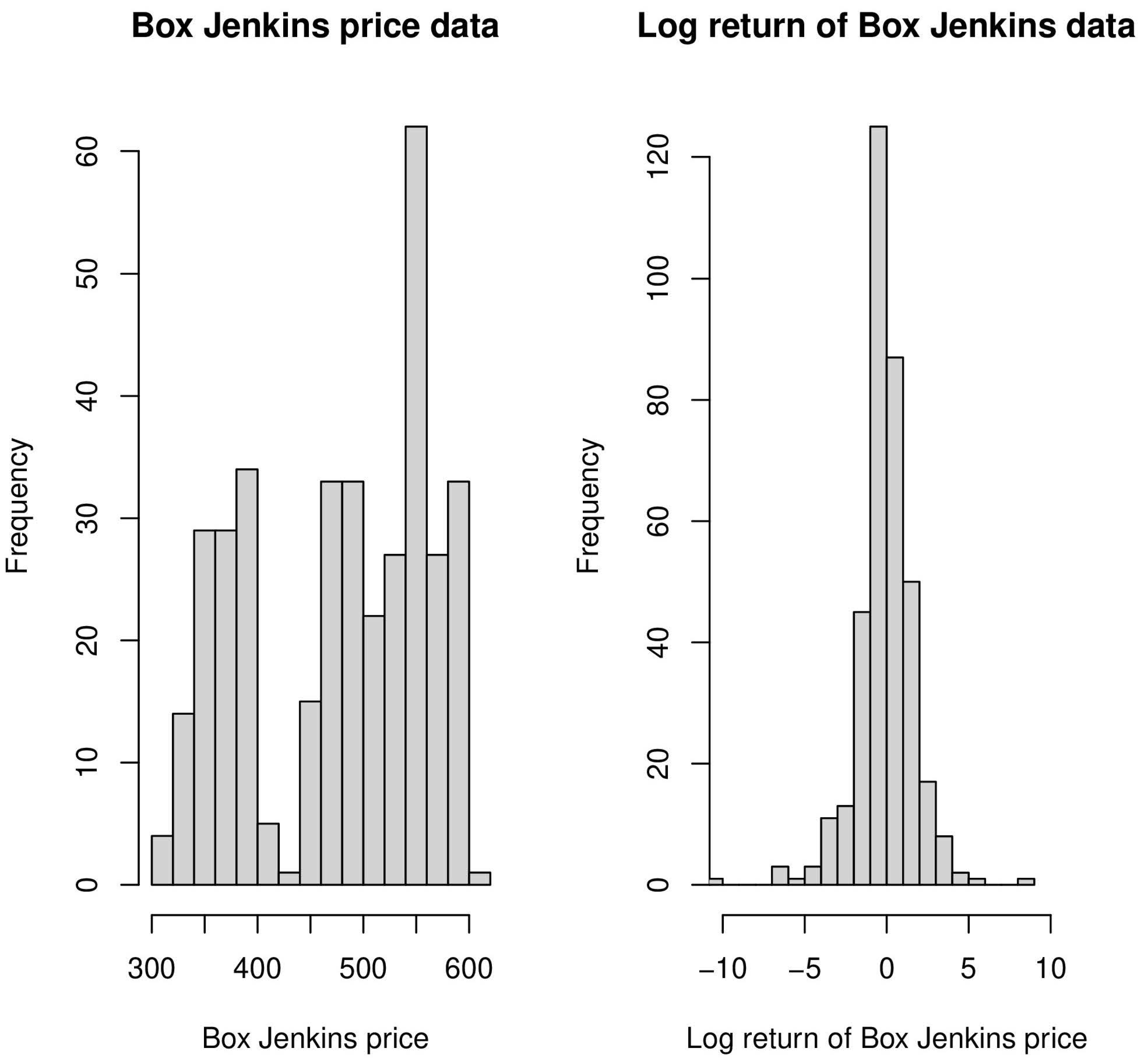
It can be observed from
Figure 1 and
Figure 2 that the distribution of the log returns of the Box–Jenkins data is, while that of the gold price data is approximately symmetric with a certain amount of left skewness, whereas the gold price data are highly skewed in nature and the Box–Jenkins price data are bimodal. Still, we have used both the gold price and Box–Jenkins log return data sets as illustrations for our proposed estimators, as well as to explore their properties. We also note that both the methods of estimation based on trigonometric moments and characteristic function are not applicable to the two price data sets, since the underlying assumptions of the model are violated by the data sets.
Table 3.
The estimates of .
Table 3.
The estimates of .
| Data | | | | |
|---|
| 1 | 1.102854 | 1.941821 | 1.27487 | 2.0 |
| 2 | 0.3752206 | 1.263993 | 0.4149459 | 2.0 |
It can be observed from
Table 3 that both the estimators are quite close to each other for the Box–Jenkins log return data, since they are symmetric in nature. The two estimators for the log return of the gold price data do not differ for wrapped stable distribution, but there seems to be an appreciable difference for wrapped Linnik distribution due to their differences in robustness against the asymmetric nature (e.g., the estimator of the location parameter by the mean and median give similar values for symmetric distribution but do not for asymmetric or skewed distribution, due to the difference in the robustness properties of the estimators). Thus, it is necessary that the assumptions of the symmetry of and independence in the data sets be verified in order to produce good estimates of the parameter by our proposed estimators as above.
11. Novel Tests for Based on Circular Statistics
We are presenting here, to the best of our knowledge, the maiden attempt of testing for the index parameter of stable and Linnik distributions. Let
be realizations of symmetric stable (
) distribution. The choice of
and
are justified, as given in
Section 3. When the sample size
n is large, we can use the asymptotic distribution of
, as stated in Theorem 5, to perform the test for the null hypothesis
. Also, since the data have undergone logarithm ratio transformation, they are thus scale invariant and hence we can take the scale parameter
in the expression of the estimator of the variance,
to perform the test. Thus, the test statistics are given by
where
denotes the trigonometric truncated moment estimator of
for the data, assuming a stable distribution.
Let
be realizations of symmetric Linnik (
) distribution. When the sample size
n is large, we can use the asymptotic distribution of
, as stated in Theorem 6, to perform the test for the null hypothesis
. Also, since the data have undergone logarithm ratio transformation, they are thu scale invariant and hence we can take the scale parameter
in the expression of estimator of the variance,
to perform the test. Thus, the test statistics are given by
where
denotes the trigonometric truncated moment estimator of
for the data assuming the Linnik distribution. Depending on the alternative hypothesis, the cut-off points of the tests can be determined from standard normal distribution tables.
A similar test can also be carried out based on a Hill estimator using Lemma 1, but it is not studied here because the determination of k is complicated.
Example:
Anderson and Arnold (
1993) have suggested the Linnik distribution for the financial data on Box–Jenkins based on their characteristic function-based method of estimation. We assume that the data come from a member of the Linnik family. In this family, the Linnik distribution is characterized by
. This has motivated us to rigorously verify their claim based on the corresponding test
against the alternative hypothesis
. As per the suggestions of the referee, we perform a test for Laplace (a.k.a. double exponential) distribution corresponding to
in the family of Linnik distributions. The test statistics as defined above are given by
The value of the test statistic is obtained as , implying that the null hypothesis of the claim of double exponential distribution is accepted both at the and levels of significance.
The Laplace distribution has been earlier used on an adhoc basis by
Anderson and Arnold (
1993) for the financial data on Box–Jenkins based on results of estimation. We have established it formally by providing rigorous proof through testing procedure which supports their findings.


