The Generalised Extreme Value Distribution Approach to Comparing the Riskiness of BitCoin/US Dollar and South African Rand/US Dollar Returns

Abstract

In this paper, the generalised extreme value distribution (GEVD) model is employed to estimate financial risk in the form of return levels and the value at risk (VaR) for the two exchange rates, BitCoin/US dollar (BTC/USD) and the South African rand/US dollar (ZAR/USD). The Basel Committee on Banking Supervision (BCBS) responsible for developing supervisory guidelines for banks and financial trading desks recommended that VaR be computed and reported. The maximum likelihood estimation (MLE) method is used to estimate the parameters of the GEVD. The estimated risk values are used to compare the riskiness of the two exchange rates and help both traders and investors to define their position in forex trading. This is to helping understanding the risk they are taking when they convert their savings/investments to BitCoin instead of the South African currency, the rand. The high extreme value index associated with the BTC/USD compared to the ZAR/USD implies that BitCoin is riskier than the rand. The BTC/USD has higher values of expected extreme/tail losses of 13.44%, 18.02%, and 23.41% at short (6 months), medium (12 months), and long (24 months) terms, compared to the ZAR/USD expected extreme/tail losses of 2.40%, 2.84%, and 3.28%, respectively. The computed VaR estimates for losses of USD 0.17, USD 0.22, and USD 0.38 per dollar invested in BTC/USD at 90%, 95%, and 99%, compared to ZAR/USD’s USD 0.03, USD 0.03, and USD 0.04 at the respective confidence levels, confirm the high risk associated with BitCoin. The conclusion drawn from this study is that BTC/USD is riskier than ZAR/USD, despite the rand being a developing country’s currency, hence perceived as being risky. The perception is that the rand is riskier than BitCoin and perceptions do influence exchange rates. Kupiec’s backtest results confirmed the model’s adequacy. These findings are helpful to investors, traders, and risk managers when deciding on trading positions for the two currencies.

1. Introduction

Cryptocurrencies are decentralised currencies that are transacted without the regulations of a reserve bank or financial intermediaries. Blockchain technology is used to process transactions. BitCoin is on top of the list of traded cryptocurrencies in terms of traded volume with a market capitalisation of USD 452.1 billion (https://www.forbes.com, accessed on 7 March 2023). Like most technical products, the uptake may be initially slow, but the above literature suggests more significant use of cryptocurrency going into the future. According to Deloitte, “more than 2300 US businesses accepted and used BitCoin, and other digital assets for a host of investment, operational, and transactional purposes in 2020” (https://www2.deloitte.com, accessed on 7 March 2023).

With the collapse of the Bretton Woods gold backed currency system (Garber 1993), the current currencies in use are viewed as fiat currencies. Fiat money is a government issued currency that is not backed by a commodity such as gold. Fiat currencies have lost some of their lustre in times of war, showing that they are not as good as gold.

Indeed, cryptocurrencies such as BitCoin are exchangeable with fiat currencies and are a faster way to exchange currency, even though some economic researchers argue that the BitCoin fails the three traditional requirements of a currency (store of value, medium of exchange, and unit of account (Yermack 2015). Lu (2023) noted that if BitCoin is accepted as a kind of new currency, it is likely that it will improve lives and help to avoid the problem of fetishism that always excludes the majority from its games.

Since BitCoin is not backed by any central bank or government, its users and traders are vulnerable to higher risk (volatility).

BitCoin is a relatively new investment asset and evidence of its use as a currency is available on the given surveys below. As with the global trend, cryptocurrency trading, particularly BitCoin, is gaining a lot of momentum in South Africa Arı (2022), (https://www.altcointrader.co.za/, accessed on 7 March 2021).Thus, according to a survey by triple A, a blockchain technology company, there is a steady increase in movements of people’s savings and investments between the rand and BitCoin (https://triple-a.io/crypto-ownership-south-africa-2022/, accessed on 5 April 2023).

Risk sentiment is how financial market participants (traders and investors) feel and behave, e.g., towards emerging countries’ currencies. The behaviour is particularly important when the economic outlook of one or some emerging countries is poor or deteriorating, economic data is disappointing or downright negative, and markets are exhibiting high levels of price volatility. Those emerging countries that maybe doing well economically may still have their currencies weakened or affected through contagion. Investors move their currencies from emerging countries to “safe haven assets” which are not affected by this negative sentiment around emerging countries.

While the rand is a government backed currency, the South African Reserve Bank (SARB) adopted a flexible exchange rate post independence in 1994 (Van Der Merwe 1996). This approach is the market driven pricing of currency, mainly based on the supply and demand of money in the market. The rand is then affected by speculation (hence perceived as being risky), foreign investor sentiment and contagion emanating from association with similar economies (Pretorius and De Beer 2002). Joale (2011, p. 4) sums it up as follows: “The reduction in controls relating to the exchange rate market and capital flows have resulted in South Africa experiencing a significant increase in the volatility of both securities (stock and bond) prices and the exchange rate of the rand against major world currencies, especially the U.S. Dollar”, and hence the perception of a very risky rand is not without merit.

Cryptocurrencies are said to be very risky (Kaseke et al. 2021). Developing countries’ currencies, including the South African rand, are equally risky (https://assets.ctfassets.net/, accessed on 18 February 2023).

Financial time series (including BitCoin and rand) are leptokurtic in nature, that is, they tend to exhibit fat tails and excess peaks from the mean (Danielsson 2011). Fat tails are responsible for extreme return; hence the use of extreme value theory (EVT) models is recommended in efforts to correctly capture the financial risk of these financial assets.EVT is the theory of measuring and modelling extreme events (large fluctuations). The field of EVT was pioneered by Fisher and Tippett (1928) and Pickands (1975). The purpose of this study is to fit the extreme value theory (EVT)-based generalised extreme value distribution (GEVD) to compare the riskiness of the two currencies by estimating return levels and the value at risk (VaR). The GEVD is preferred as it analyses extreme risk. Edem and Ndengo (2021) showed that GEVD adequately captures tail-related features for financial indices in developing economies such as Rwanda.

In the modelling of financial extreme tail-related risk using the EVT, the extreme value index (EVI), also known as the shape parameter of the distribution, dictates the tail behaviour of the returns’ distribution, according to Rached and Larsson (2019). This parameter is so important and is an indicator of how the tail of a distribution decays, according to Beirlant et al. (2005). A lot of studies have been carried out to refine the methods of estimating EVI. Work includes Dekkers et al. (1989), Beirlant et al. (1996, 2005), Caeiro et al. (2005), and Cai et al. (2013). The parameter itself is a measure of risk when working with the EVT as loss distributions, and it also influences the estimation of risk measures such as return levels, value at risk (VaR), and expected shortfall (ES) (Penalva et al. 2016).

The return level is defined as, say, the maximum loss (exceedance) over an average period of, say, one year. It measures the highest (extreme quantile) to occur within a certain period. Therefore, the return value is the level that is expected to be equalled or exceeded on average once every interval of time with a probability of p (McNeil et al. 2015). Jakata and Chikobvu (2022) defined the waiting time as “the waiting period before observing a maximum loss of the same magnitude”. Gilli and Këllezi (2006) suggested that the maximum loss of an investment portfolio can be better estimated by the return value (level), rather than the more conservative measure of the VaR.

The VaR is a statistic that quantifies the riskiness of a financial portfolio of assets. It is the largest value or amount expected to be lost over a specified time horizon, i.e., daily, weekly, or ten days, at a pre-defined statistical confidence level. Hull (2006, p. 198) defined VaR as the value that “compresses all Greek letters for all the market variables underlying a portfolio into a single number”. Investors and practitioners rely heavily on VaR as a risk measure, even though it is not globally sub-additive. The VaR metric is popular because its practical advantages outweigh its theoretical disadvantages. According to Danielsson et al. (2013), VaR is sub-additive in most practical situations, which is in line with the diversification concept of modern portfolio theory.

This paper compares the riskiness of the BitCoin returns with the South African rand returns using GEVD-based return levels and VaR. The theory of extremes is backed by mathematical theory and governs the behaviour of extremes (outliers). Just as the central limit theorem governs the normal distribution behaviour of data when a large data set is available, Fisher and Tippett (1928) and Pickands (1975) proved a similar theorem for those extremes (outliers).The theorem applies to a population that may exhibit extremes. The normal distribution-based models have been discredited, as they are largely blamed for the global financial crisis of 2008/9. The originality of the work in this paper should be viewed within the context of applying already established statistical distributions to compare extreme risk in BitCoin and rand returns. Similarities and hence conclusions to other developing countries can be inferred, but each developing country’s currency warrants a separate study and hence a separate conclusion.

The paper provides scarce empirical evidence when comparing a risky developing country’s currency, the rand, to BitCoin. The normal distribution-based model empirical evidence is discredited in favour of extreme value theory (EVT) distributions through empirical evidence, such as that provided using the GEVD model.

The rest of the paper is organised as follows: Section 2 presents the literature review. The methodology is in Section 3. Results and discussions are in Section 4 and Section 5 concludes.

2. Literature Review

Dasman (2021) used a statistical test approach in comparing the average returns and volatility of BitCoin against the Indonesian Composite Index, and gold. The BitCoin average returns were significantly higher than the financial assets studied. This would be consistent with mean-variance portfolio theory, which suggests a higher yield for riskier assets (Markowitz 1959).

Other studies confirmed the highly volatile nature of cryptocurrency, including Zhang et al. (2018), Katsiampa et al. (2019), and Hu et al. (2019). This feature has been suggested to be caused by speculation (perceived as being risky), insufficient regulatory measures, and spurious issues, amongst other reasons given by Dowd (2014), and Cheah and Fry (2015). However, Blau (2017), found no evidence of speculation as the reason for the high volatility amongst cryptocurrencies.

While the issue of fat tails has been raised long before the global financial crisis of 2008, such as in the work of Mandelbrot (1963) and Fama (1963, 1965), the widespread implementation in practice has lagged behind till post the global financial crisis (Danielsson 2011), (Makhwiting et al. 2014) and (Makatjane and Moroke 2021). Cirillo and Taleb (2020) emphasised the importance of fat-tailed models in extremes driven by disasters such as pandemics, e.g., the COVID-19 pandemic. An extreme asset price change can significantly affect the performance of an investment over a long time period (e.g., a year) or even threaten the stability of the whole financial market system, and hence should not be downplayed in any serious policy discussion, according to Taleb (2020).

While the value at risk (VaR) is one of the most commonly used risk measures in finance because of its ability to compress all Greeks to a single value, it has shortcomings according to Chou and Wang (2014) and, Hull (2006). Rockafellar and Uryasev (2002) showed that the traditional normal distribution-based VaR is not only incoherent, but also fails to precisely estimate the risk of loss when the loss distributions have ‘fat tails’ unless EVT distributions are used. “This significantly discredits the accuracy of the traditional normal distribution based VaR risk measure” according to Chen (2018). To address the normal distribution-based VaR weaknesses highlighted above, the EVT theory-based GEVD is suggested in this study.

As an alternative, modelling return levels as a risk measure has been used increasingly in geophysical sciences and financial analysis (Chifurira 2018), (Maposa 2016). Musara et al. (2022) used probability plots, quantile plots, and Kolmogorov–Smirnov tests to confirm the model adequacy of GEVD-based return levels as a measure of risk.

There has been an increase in the amount of research to ascertain whether the stylised facts of cryptocurrency are similar to those of other financial assets. Arı (2022) showed that the Levy-driven continuous-time GARCH model shows a better performance in predicting volatility than the discrete-time GARCH. Kaseke et al. (2021) showed that cryptocurrencies have similar distributional characteristics with gold and the FTSE/JSE 40, although the cryptocurrency is more volatile. Takaishi (2018) noted the presence of heavy-tailedness and excess kurtosis in the one-minute returns data of BitCoin. Bouri et al. (2017) observed a high negative skewness and volatility in BitCoin in comparison to other stock returns.

Malladi (2022) used five econometric methods (pooled ordinary least square regression model, fixed-effects model, random-effects model, panel vector error correction model, and generalized autoregressive conditional heteroskedasticity model) to model cryptocurrencies’ volatility and price linkage to other assets classes (such as gold, stocks, and bond markets) and found that the panel vector error correction model fits best. Furthermore, he found that cryptocurrencies exhibit negative alpha, and high beta (riskiness), similar to stocks from emerging markets.

Dyhrberg (2016) argued that the shocks that are prevalent in the financial market do not affect BitCoin and gold returns; hence they can be used for hedging. Conversely, Shanaev and Ghimire (2021) noted relative stability in BitCoin and Ethereum using asymmetric power-law statistical distributions.

This paper uses the GEVD model to compare the riskiness of the BitCoin and the South African rand returns at the extremes/tails of statistical distributions of the returns. Both currencies are measured against the US dollar. The steady rise in the movement of people’s investment between the rand and BitCoin since the introduction of cryptocurrency influenced the selection of the two financial assets. The GEVD model allows for the analysis of extreme gains and losses that may be associated with investing in BitCoin. The rand is also another developing country’s currency which is considered to be very risky. By analysing the extreme gains and losses, this research’s aim is to ascertain which of the two currencies is riskier and use the findings to help investors understand the risk they are taking when they convert their savings/investments to BitCoin instead of the South African currency, the rand. This helps forex traders, risk managers and others to choose their optimal trading position.

3. Methodology

The theory of extremes is backed by mathematical theory and governs the behaviour of extremes (outliers). Just as the central limit theorem governs the normal distribution behaviour of data when a large data set is available, Fisher and Tippett (1928) and Pickands (1975) proved a similar theorem for those extremes (outliers).The theorem applies to a population that may exhibit extremes. The GEVD is a result of the application of the Fischer–Tippet theorem; simply put the theorem says, as the sample size is slowly increased, the maxima or minima of that sample will always follow asymptotically, the GEVD.

The block maxima (BM) method is an EVT approach for identifying the maximum/minimum (extremes) in a data set and models their behaviour, according to Gumbel (1958). Suppose $Y_1,Y_2,\dots ,Y_n$ represents the independent and identically distributed log returns of an asset’s index. Then, for maximum values/gains:

$$M_n=\max [Y_1,Y_2,\dots ,Y_n]$$

(1)

For the minimum values (losses):

$$m_n=\min [Y_1,Y_2,\dots ,Y_n]=-\max [{-Y}_1,-Y_2,\dots ,{-Y}_n]$$

(2)

Losses are negative returns which have been converted into positive values by multiplying by negative one (−1). $M_n$ and $m_n$ are the maxima over an n-observation period.

Suppose we find normalising sequences of real numbers $\left(c_n\right)>0$ and $\left(d_n\right)$ such that

$(M_n-d_n)/c_n$ converges to a distribution as follows:

$$\begin{array}{ll}\mathbb{P}(M_n–d_n)/c_n\le y)& =\mathbb{P}(M_n\le c_{n}y+d_n)\\ & =\mathbb{P}\left(Y_i\le c_{n}y+d_n,i=\mathrm{1,2},..,n\right)\\ & {=F}^n\left(M_n\le c_{n}y+d_n\right)\underset{n\uparrow \infty }{\to }G(y)\end{array}$$

For the non-degenerate distribution function $G$ (not a unit jump), $F$ is in the maximum domain of attraction, i.e., $(F\in MDA(G\left)\right)$. Fisher and Tippett (1928) and Gnedenko (1943) showed that $G\left(y\right)$ is a limiting distribution of normalised maxima of a sequence of independent, identically distributed random variables as follows.

$$G(y)=\left\{\begin{array}{c}\exp \left(-{\left(1+\xi y\right)}^{-\raisebox{1ex}{$1$}\!\left/ \!\raisebox{-1ex}{$\xi $}\right.}\right),\mathrm{if} \xi \ne 0\\ \exp \left(-e^{-y}\right),\mathrm{if} x\ge 0\end{array}\right.$$

(3)

A three-parameter family statistical distribution is obtained by a location-scale transform.

$$G_{\xi ,\mu ,\sigma }\left(y\right)=G_{\xi }\left(\frac{y-\mu }{\sigma }\right),\mu ϵ\mathbb{R},\sigma >0,1+\xi \left(\frac{y-\mu }{\sigma }\right)>0.$$

where $\mu$ and $\sigma$ are the location and scale parameters, respectively. The shape parameter $\xi$ is also known as the extreme value index (EVI).

The probability density function, obtained as the derivative of the above distribution function, is given as

$$g_{\xi ,\mu ,\sigma }\left(y\right)=\frac{1}{\sigma }{\left(1+\xi \left(\frac{y-\mu }{\sigma }\right)\right)}^{-1-\raisebox{1ex}{$1$}\!\left/ \!\raisebox{-1ex}{$\xi $}\right.}\exp \left\{-{\left(1+\xi \left(\frac{y-\mu }{\sigma }\right)\right)}^{-\raisebox{1ex}{$1$}\!\left/ \!\raisebox{-1ex}{$\xi $}\right.}\right\},\mathrm{i}\mathrm{f} \xi \ne 0$$

(4)

$$g_{\xi ,\mu ,\sigma }\left(y\right)=\exp \left(-\frac{y-\mu }{\sigma }\right)\exp \left(-\exp \left(-\frac{y-\mu }{\sigma }\right)\right),\mathrm{i}\mathrm{f} \xi =0$$

(5)

The log-likelihood for the parameters, when $\xi \ne 0$, is

$$l\left(\xi ,\mu ,\sigma \right)=-n\ln \left(\sigma \right)-\left(1+\frac{1}{\xi }\right)\sum _{i=1}^n\mathrm{l}\mathrm{n}\left[1+\xi \left(\frac{y_i-\mu }{\sigma }\right)\right]-\sum _{i=1}^n{\left[1+\xi \left(\frac{y_i-\mu }{\sigma }\right)\right]}^{-\frac{1}{\xi }}$$

(6)

when $\xi =0$

$$l\left(\xi ,\mu ,\sigma \right)=-n\ln \left(\sigma \right)-\sum _{i=1}^n\left(\frac{y_i-\mu }{\sigma }\right)-\sum _{i=1}^n\mathrm{e}\mathrm{x}\mathrm{p}\left(\frac{y_i-\mu }{\sigma }\right)$$

(7)

According to Coles (2001), maximisation of the above function with respect to the parameters vector $\left(\xi ,\mu ,\sigma \right)$, leads to the MLEs for the entire GEVD family.

3.1. Return Level

Jakata and Chikobvu (2022, p. 305) cited Gilli and Këllezi’s (2006) description of a return level as “a better measure of maximum loss of an investment portfolio rather than the more conservative measure of VaR”.

The return level as a risk measure is the value ($y_T$) of the return expected to occur in one out of $T$ periods of length $n$, and is by definition

$$\begin{gathered} R_n^T=\mathbb{P}\left(Y>y_T\right)=\frac{1}{n^T} \\ \begin{array}{ll}\mathbb{P}\left(Y\le y_T\right)& =1-\frac{1}{n^T}\\ & =G^{-1}\left(1-\frac{1}{n^T}\right)\end{array} \end{gathered}$$

where n is the average number of extremes per $T$ periods of length, and for GEVD can be summarised as

$$R_n^T=\left\{\begin{array}{c}\widehat{\mu }-\left(1-\frac{\widehat{\sigma }}{\widehat{\xi }}\left(1-\left(\ln {\left(1-\frac{1}{n^T}\right)}^{-\widehat{\xi }}\right)\right)\right)\\ \widehat{\mu }-\left(1-\widehat{\sigma }\ln \left(-\ln \left(1-\frac{1}{n^T}\right)\right)\right)\mathrm{i}\mathrm{f} \widehat{\xi }=0\end{array}\right.\mathrm{i}\mathrm{f} \widehat{\xi }\ne 0$$

(8)

where $\widehat{\mu }$, $\widehat{\sigma }$ and $\widehat{\xi }$ are estimates from the GEVD model.

3.2. Value at Risk

McNeil et al. (2015) showed that the formula for computing the value at risk, for a small tail probability $p$, and total sample size $n$, for a GEVD with maximum likelihood estimates $(\widehat{\mu },\widehat{\sigma },\widehat{\xi })$ can be expressed as

$$\widehat{{VaR}_p}=\left\{\begin{array}{c}u+\frac{\widehat{\sigma }}{\widehat{\xi }}\left\{{\left(\frac{n}{N_u}p\right)}^{-\widehat{\xi }}-1\right\}\mathrm{i}\mathrm{f} \widehat{\xi }\ne 0\\ u-\widehat{\beta }\ln \left(\frac{n}{N_u}(1-p)\right)\mathrm{i}\mathrm{f} \widehat{\xi }=0\end{array}\right.$$

(9)

and $N_u$ is the number of blocks.

3.3. Backtesting

To validate the model adequacy and effectiveness in the computation of VaR used to compare the two currencies, the Kupiec unconditional coverage test by Kupiec (1995) is used. It is preferred due to its simple but effective ability to guarantee model adequacy (Zhang and Nadarajah 2017). Other techniques such as the Christoffersen conditional coverage test by Christoffersen (1998) goes further to test the clustering of model violations. However, Haas (2001) argues that the Christoffersen test is too weak to produce feasible results.

The unconditional coverage test by Kupiec assumes that the proportion of violations of VaR estimates must be close to the corresponding tail probability level if the model is adequate.

Let $x^p$, be the number of violations observed at level p, i.e., $r_t<{VaR}_p$ (for long positions) or $r_t>{VaR}_p$, (for short positions). The test procedure involves comparing the corresponding proportion of violation [$\frac{x^p}{N}$] to p. The H₀: E$\left[\frac{x^p}{N}\right]=p$ i.e., the expected proportion of violations is equal to $p$.

Under H₀, the Kupiec likelihood ratio test is

$${LR}_{UC}=-2\mathit{ln}\left(\frac{p^{x^p}{\left(1-p\right)}^{N-x^p}}{{\left(\frac{x^p}{N}\right)}^{x^p}{\left(1-\frac{x^p}{N}\right)}^{N-x^p}}\right),$$

(10)

and it follows a chi-square distribution with one degree of freedom, and N is the total observations. We reject H₀ if the Kupiec statistic is greater than the critical value (chi-squared) or p value is less than the p statistic. If the null hypothesis is rejected, it can be concluded that model estimates are significantly different from what is expected.

4. Results Analysis and Discussion

Currency data used in this research was obtained from the finance sector website (www.investing.com/currencies, accessed on 1 July 2021). Analysis was conducted using R (R Core Team 2021), RStudio (RStudio Team 2022), evir (Pfaff and McNeil 2018), rugarch (Ghalanos 2020), ismev (Heffernan and Stephenson 2018) and eva (Bader and Yan 2020) statistical packages. The adjusted closing values of daily exchange rates from 1 January 2015 to 30 June 2021 were fitted to the GEVD model. BitCoin is traded every day, hence there are 2370. The rand is not traded on weekends and South Africa’s public holidays, resulting in 1694 observations. To align our data for analysis, we replaced missing values in the rand exchange rate with zero, since there are no profits or losses realised by the holder of the local currency during the weekend and/or public holidays. The daily log returns were calculated and used for modelling. The formula used is $y_t=\log \left[\frac{P_t}{P_{t-1}}\right],$ where $P_t$ and $P_{t-1}$ are todays’ and yesterdays’ closing values of daily prices (exchange rates), respectively.

In Figure 1 and Figure 2, the log returns are stationary, around the zero-mean, although volatility is non-constant and clustered, indicating heteroscedasticity, which is common with financial data. Isolated extreme returns are visible, and are caused by shocks in the financial markets.

Descriptive Statistics

Table 1. Descriptive statistics of exchange rate price returns.

	Observations	Mean	Median		Maximum	Minimum	Skewness		Kurtosis
BTC/USD	2370	0.001990	0.001757		0.237220	−0.480904	−0.994382		16.15451
ZAR/USD	1694	−0.000125	0.000000		0.049546	−0.048252	−0.264130		4.121644
Test for Normality, autocorrelation and heteroscedasticity
		BTC/USD				ZAR/USD
TEST		Statistic		p-value		Statistic		p-value
Jarque-Bera		17,478.40		0.000000		108.4967		0.000000
Ljung-Box		11.7		0.0006249		0.40504		0.5245
ARCH LM Test		52.87		$4.345 \times$ 10−7		70.789		$2.28 \times$ 101
Test for unit root and stationarity
		BTC/USD				ZAR/USD
Unit Root Test		Statistic		p-value		Statistic		p-value
ADF Test		−52.20130		0.0001		−40.47263		0.0000
PP Test		−52.10963		0.0001		−40.47011		0.0000
KPSS Test		0.092067		0.347000		0.090747		0.347000

below presents the descriptive statistics.

In Table 1 the null hypothesis of normality using Jarque–Bera is rejected at the 5% level of significance, meaning the use of symmetric models should not be considered when analysing the above-mentioned return series.

The significant $p$-value of the Ljung–Box test for ZAR/USD returns suggest the failure to reject the null hypothesis of no autocorrelation. This means observations can be assumed to be independent and identically distributed (i.i.d). However, for the BTC/USD returns, this null hypothesis is rejected, hence a block maxima approach will therefore be used to help deal with the autocorrelation problem. The BM approach reduces this autocorrelation.

The stationarity tests (ADF and PP) show that, at the 5% level of significance, the null hypothesis of a unit root is rejected and it can be concluded that both exchange rate return series are stationary. The KPSS test results showed that all returns are stationary as well.

The gains and losses are analysed separately. The monthly period minima/maxima were extracted from the daily returns of the BTC/USD and ZAR/USD returns data using the BM method. The gains (maxima) and losses (minima) were fitted to the GEVD separately. The fitted models were used to estimate the parameters ($\widehat{\xi }$, $\widehat{\sigma }$ and $\widehat{\mu }$) and to estimate VaR as well as the return levels as a measure of tail-related risk.

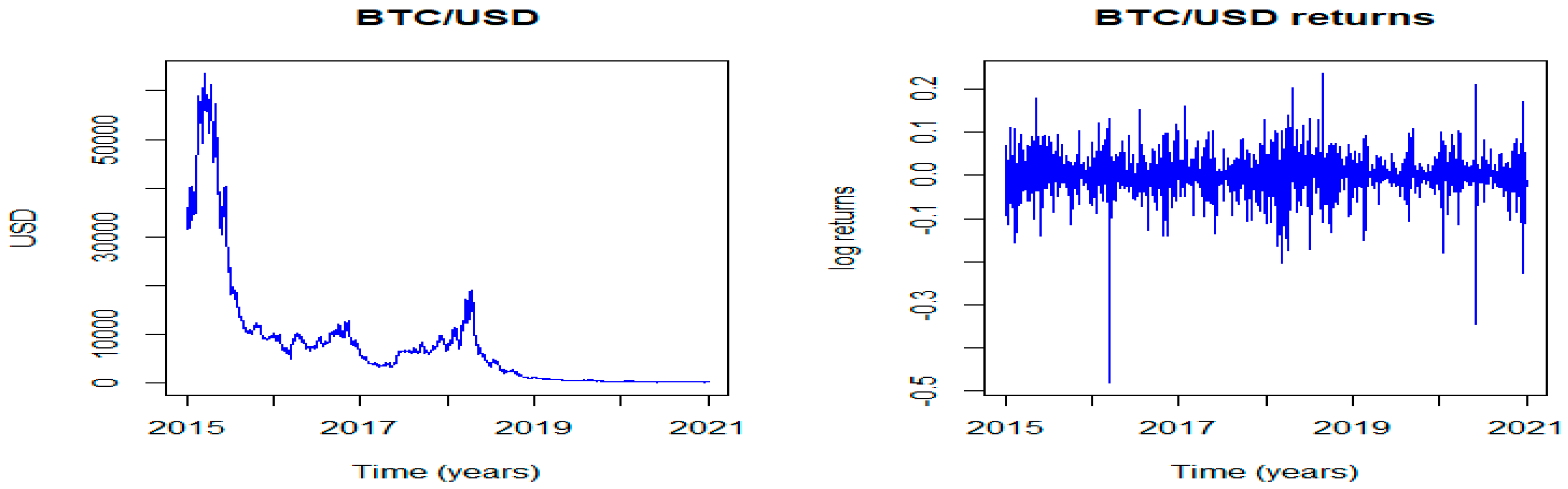
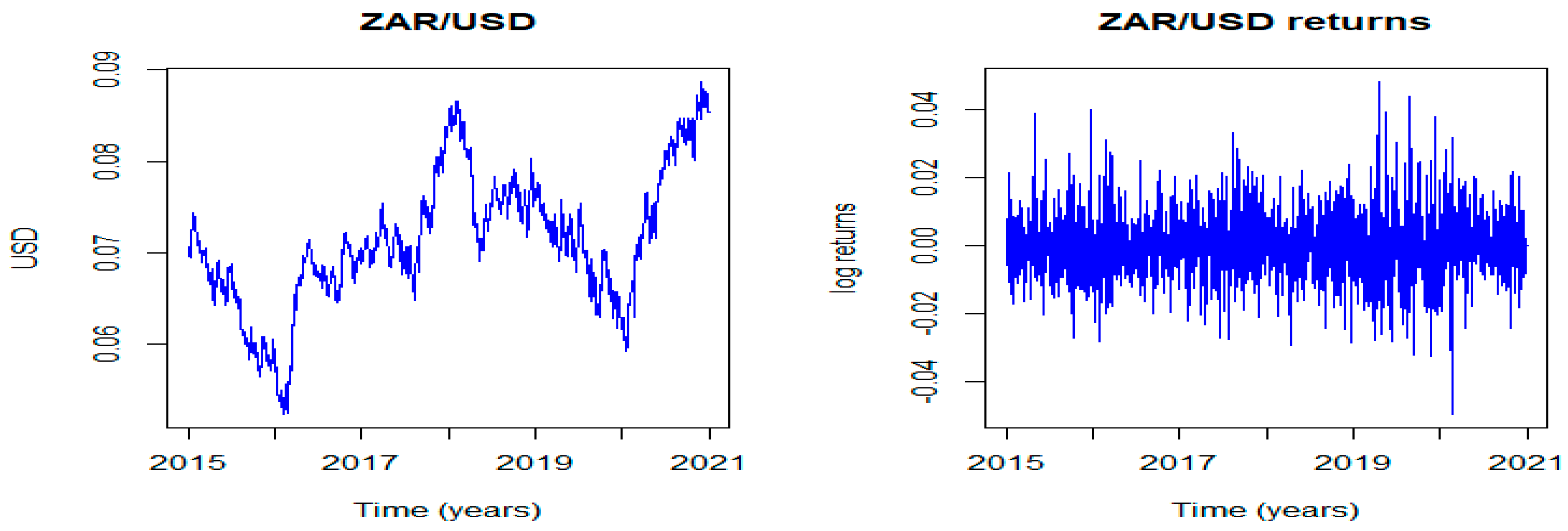
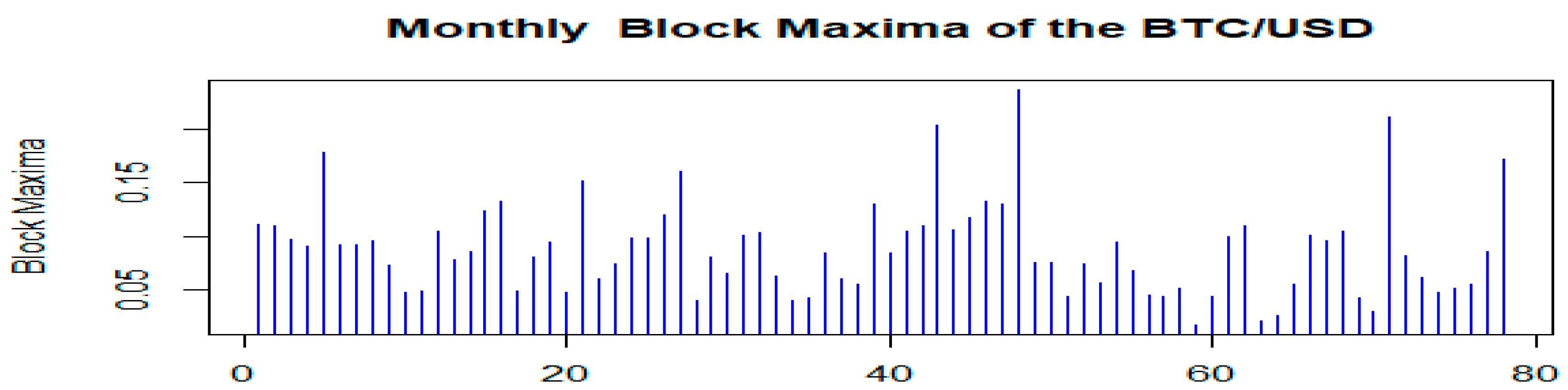
4.1. Analysing the Gains of BTC/USD and ZAR/USD

In order to get the block maxima of gains, the BitCoin returns data were put into monthly blocks. The maximum value in each block/month was selected and retained for further analysis.

The selected monthly BitCoin maxima (gains) are shown on a graph in Figure 3. The maximum value in each block/month was selected and retained for further analysis.

The selected monthly rand maxima (gains) are shown on a graph in Figure 4.

The gains of the two currency exchange rates selected from the monthly block maxima are used to estimate the GEVD parameter estimates.

In Figure 5 we present the graphical goodness of fit plots for BitCoin returns. The probability and quantile plots are almost linear, confirming a good fit. The return levels are within the confidence bands as expected. The density plot is also a good estimate to the histogram of the data. The model does fit the BitCoin gains data well.

In Figure 6, the graphical diagnostic plots show that the probability and quantile plots and rand returns also do not deviate much from the straight line, suggesting that the GEVD model is ideal for rand returns. The return level plots indicate that there are no significant deviations from the given confidence level band. The density plot is a good estimate of the histogram of the rand gains data.

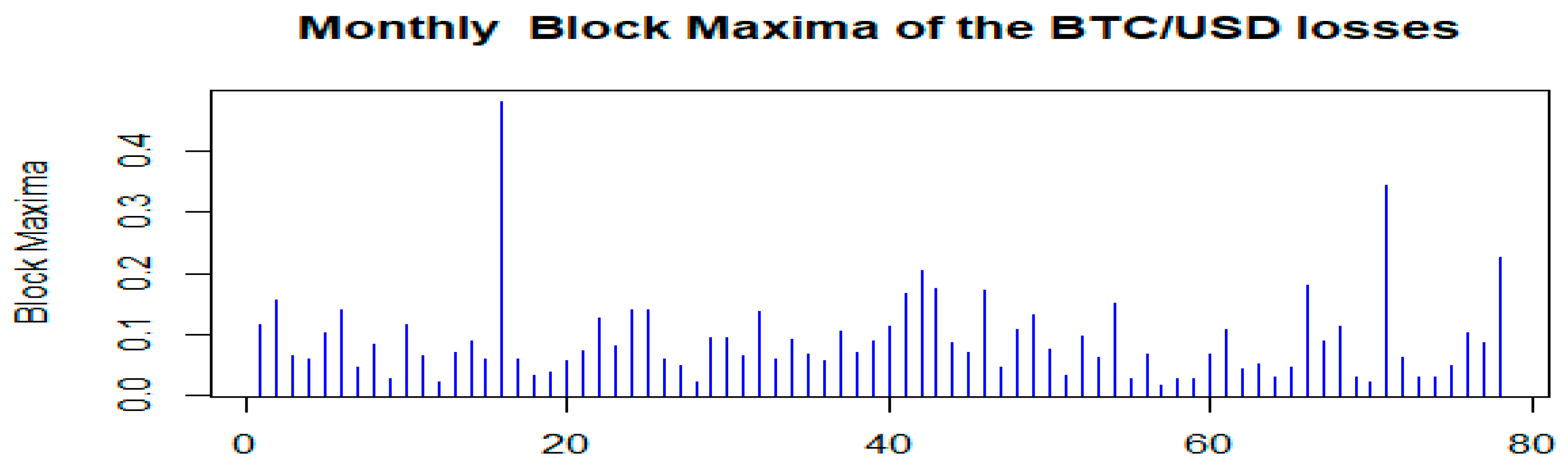
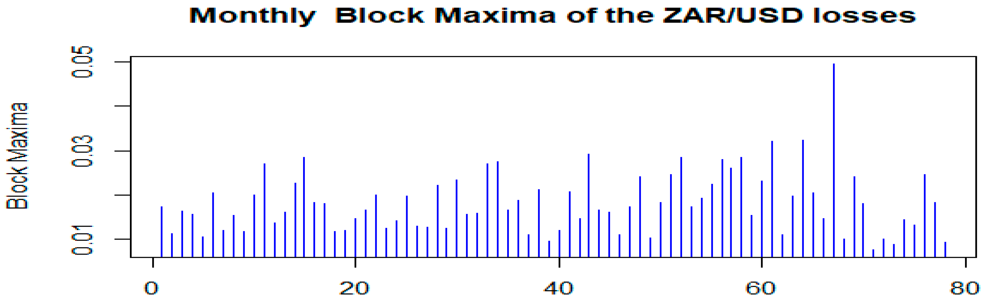
4.2. Analysing Losses for the BTC/USD and ZAR/USD

To obtain to the losses, the data are transformed using the formula $l_t=-1\ast y_t.$ Monthly maxima are again selected from these losses to come up with a new set of losses, much smaller in quantity/size, of the data set.

The selected monthly BitCoin maxima losses are depicted in Figure 7.

Similarly, to get the block maxima for the rand, the losses are transformed using the formula $l_t=-1\ast y_t$ and put into monthly blocks. The maximum value in each block was selected and retained for further analysis. The peaks in this new transformed data set represent maximum losses.

The selected monthly rand maxima losses are depicted in Figure 8. The maxima of losses are then used to fit the GEVD. Figure 7 and Figure 8 give the graphical goodness of fit measures for the losses.

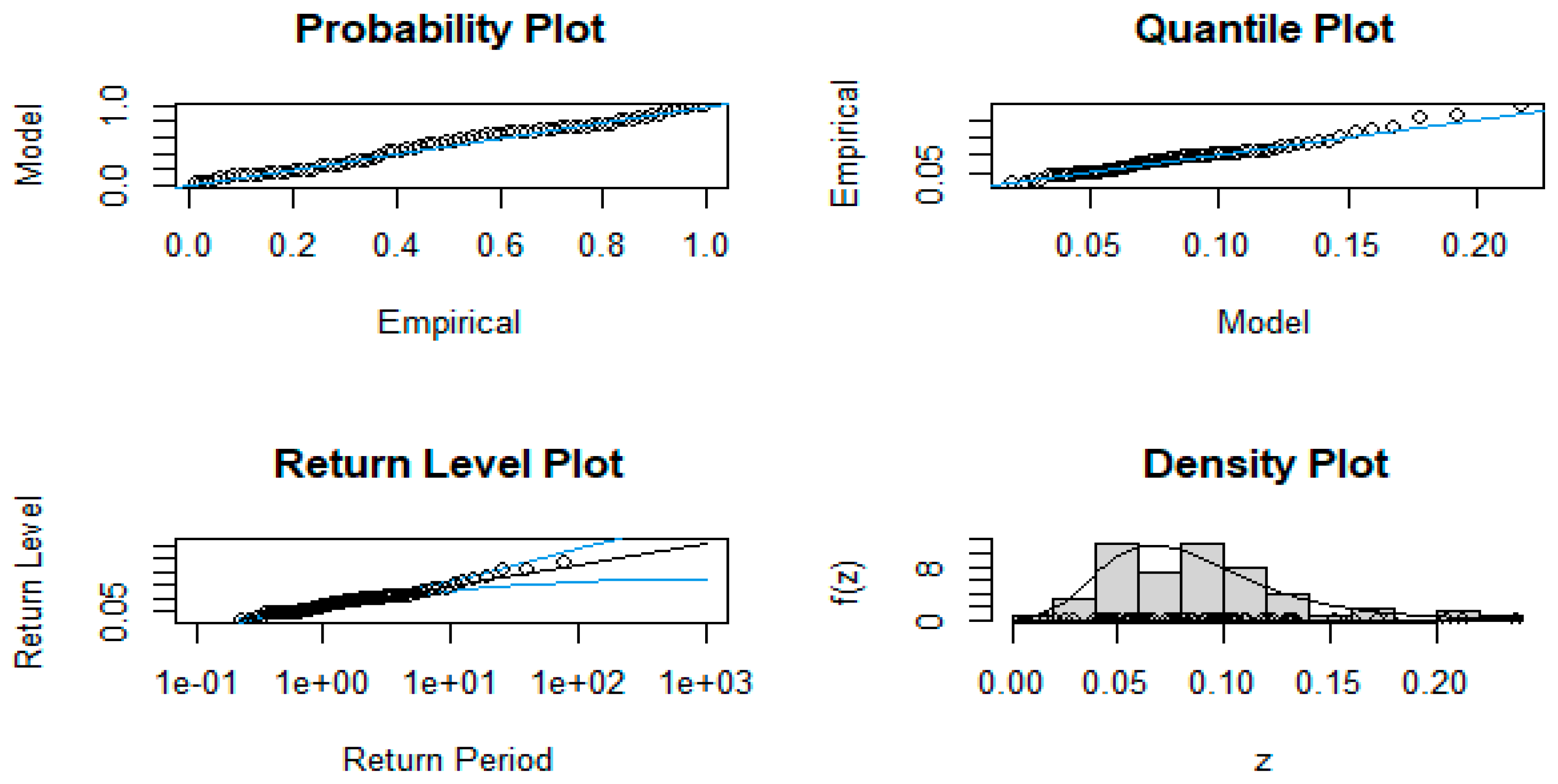
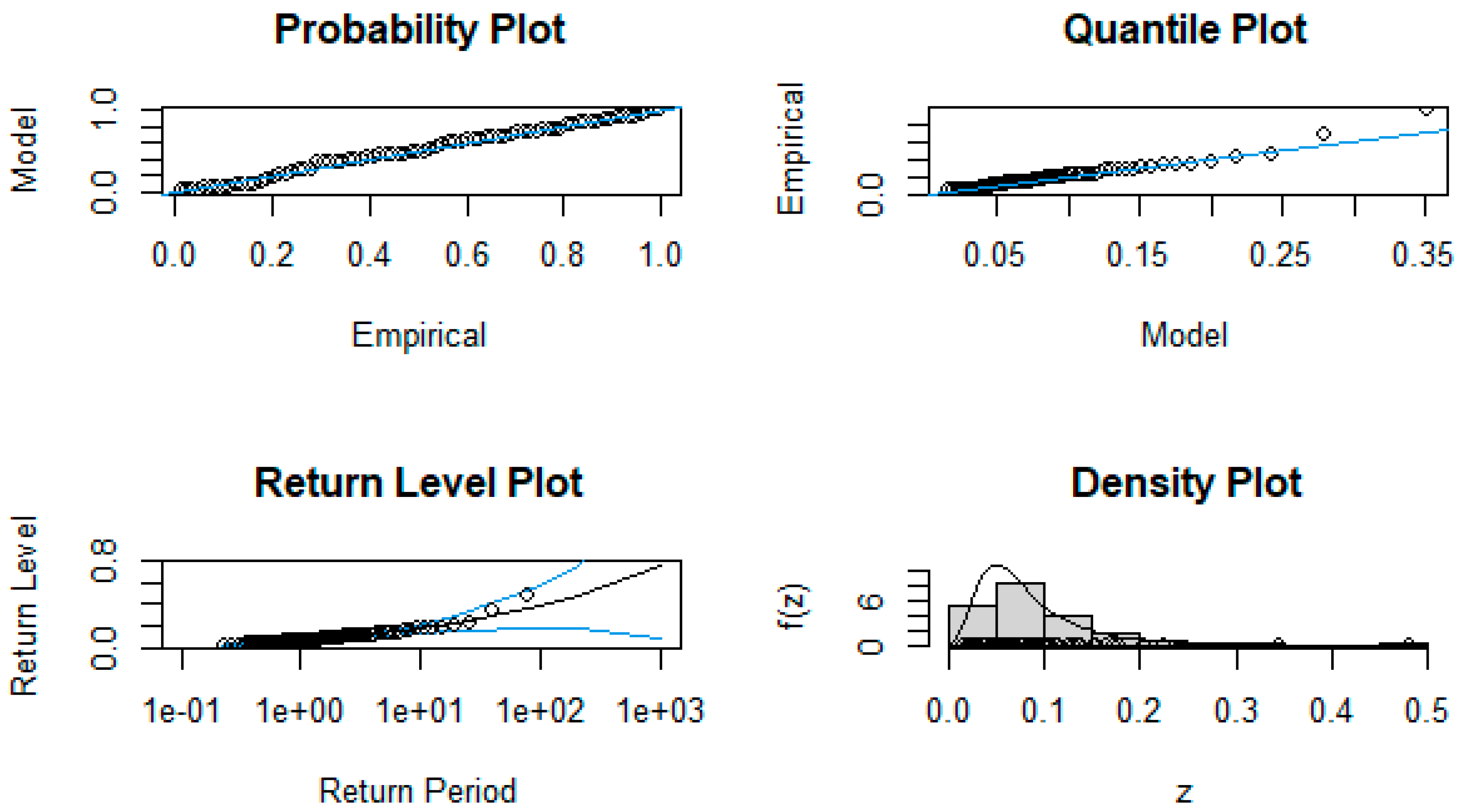
4.3. Model Diagnostics for the Maxima of the BTC/USD (Lower Tail, Loses or Minima Returns)

In Figure 9, the probability and quantile plots for the BitCoin returns do not deviate much from the straight line, suggesting that the GEVD model is ideal for BitCoin losses. The return level plots indicate that there are no significant deviations from the given confidence level band. The density plot is a good estimate of the histogram of the BitCoin losses data.

The diagnostic plots in Figure 10 confirm that the GEVD model is ideal for the rand currency losses.

4.4. Parameter Estimations

The block maxima of both currencies’ returns are fitted to GEVD with monthly block sizes.

Table 2. Parameter estimates using maximum likelihood estimator for GEVD.

Model	Maxima	$\widehat{\mathit{\xi }}$	$\mathit{S}\mathit{e}\mathit{S}\mathit{e}\left(\widehat{\mathit{\xi }}\right)$	$\widehat{\mathit{\sigma }}$	$\mathit{S}\mathit{e}\mathit{S}\mathit{e}\left(\widehat{\mathit{\sigma }}\right)$	$\widehat{\mathit{\mu }}$	$\mathit{S}\mathit{e}\mathit{S}\mathit{e}\left(\widehat{\mathit{\mu }}\right)$
BTC/USD Gains	78	0.0212	0.08501	0.03289	0.00306	0.06764	0.00421
ZAR/USD Gains	78	0.0076	0.08187	0.00656	0.00053	0.01660	0.00084
BTC/USD Losses	78	0.2699	0.11185	0.03537	0.00388	0.05796	0.00469
ZAR/USD Losses	78	0.0694	0.09586	0.00507	0.00040	0.01490	0.00066

shows the MLEs of the parameters and their corresponding standard errors (SE) for both gains and losses.

All EVIs ($\widehat{\xi }\mathrm{’}\mathrm{s}$) are positive, implying that both gains and losses for the two exchange rates follow a heavy tail Fréchet class distribution (Penalva et al. 2016). This parameter estimate confirms data sets are heavy-tailed. In both cases, gains and losses, the BTC/USD has greater index values i.e., on the gains BTC/USD has $\widehat{\xi }$ of 0.0212 compared to rand’s $\widehat{\xi }$ of $0.0076$, also on the losses the BTC/USD has $\widehat{\xi }=0.2699$ compared to ZAR/USD’s $\widehat{\xi }=0.0694$. These EVIs leads one to conclude that the BitCoin is riskier than the South African rand (for the period understudy) from both sides of the trader’s long and short positions. Both currencies have heavier tails on the losses than on the gains.

4.5. Return Levels Estimates

In

Table 3. Return levels estimates using the fitted GEVD model.

	BTC/USD			ZAR/USD
	Lower Bound of Return Level	Point Estimate	Upper Bound of Return Level	Lower Bound of Return Level	Point Estimate	Upper Bound of Return Level
	GAINS			GAINS
6 months	0.11	0.12	0.14	0.03	0.03	0.03
12 months	0.13	0.15	0.18	0.03	0.03	0.04
24 months	0.15	0.18	0.22	0.03	0.04	0.05
	LOSSES			LOSSES
6 months	0.11	0.13	0.17	0.02	0.02	0.03
12 months	0.15	0.18	0.25	0.03	0.03	0.03
24 months	0.18	0.23	0.36	0.03	0.03	0.04

, for the BTC/USD, the expected tail-related losses of 13.44%, 18.02%, and 23.42% at short (6 months), medium (12 months), and long (24 months) terms, respectively, are greater than the expected tail-related gains of 12.46%, 15.00%, and 17.50%.

Based on these results, a short position (selling a BitCoin today and buying it back at a later date) is recommended rather than a long position (holding a BitCoin hoping to sell it at a later date at a higher price) since there is a higher chance of realising a loss than a gain in the long run when holding a BitCoin.

For ZAR/USD, the expected tail-related gains of 2.78%, 3.28%, and 3.75% at short (6 months), medium (12 months), and long (24 months) terms, respectively, are greater than the expected tail-related losses of 2.40%, 2.84%, and 3.28%. Hence a long position (holding a unit of rand hoping to sell it on a later date at a higher price) is recommended rather than a short position (selling a unit of rand today and buying it back at a later date) since there is a higher chance of realising a gain than a loss in the long run when holding a rand.

4.6. Value at Risk Estimates

The VaR estimates using the GEVD model are summarised in

Table 4. VaR estimates.

	BTC/USD		ZAR/USD
	Losses	Gains	Losses	Gains
90%	0.17	0.14	0.03	0.03
95%	0.22	0.17	0.03	0.04
99%	0.38	0.23	0.04	0.05

.

The computed values suggest that the BTC/USD is riskier than the ZAR/USD for both gains and losses since it has a higher value at risk per US dollar invested in each currency. Losses of USD 0.17, USD 0.22, and USD 0.38 per dollar invested in BTC/USD at 90%, 95%, and 99% compared to ZAR/USD’s losses of USD 0.03, USD 0.03, and USD 0.04 at the respective levels of significance, confirm the high risk associated with BitCoin.

Comparing losses to gains for BTC/USD, the results indicate that the prospects of potential extreme losses are greater than the prospects of potential extreme gains. Comparing losses to gains for ZAR/USD, the results indicate that the prospects of potential extreme gains are greater than the prospects of potential extreme losses.

4.7. Backtest Results

The VaR estimates from the fitted GEVD model are backtested using the Kupiec test. The $p$-values greater than 5% imply that the model adequacy is achieved.

Table 5. Kupiec backtest results.

	BTC/USD		ZAR/USD
	Losses	Gains	Losses	Gains
90%	0.76	0.76	0.66	0.94
95%	0.63	0.58	0.63	0.31
99%	0.81	0.81	0.81	0.81

summarises the findings.

Based on the Table 4 above, GEVD fits fairly well to both BTC/USD and ZAR/USD currency series’ gains and losses, hence model adequacy is accepted in all cases as the p-values are greater than the 5% significance level.

5. Discussion and Conclusions

In this study, the GEVD model is employed to estimate return levels and VaR and are used to compare the riskiness of the BitCoin and South African rand, both indices measured against the US Dollar. Both exchange rates exhibited heavy-tail behaviour in gains and losses, providing a good fit to the tails of the distributions. The shape parameter for instance, which is a useful tool for checking how heavy the tails are, gave values greater than zero, signifying the GEVD is the heavy tail type Fréchet class distribution (Penalva et al. 2016). This demonstrates the existence of heavy-tailedness or the presence of extremes (outliers). The EVT model provided a good fit to the tails of the distribution of the returns. The diagnostic plots showed that the probability and quantile plots do not deviate significantly from a straight line, signifying a good fit.

In Table 2, the higher expected tail-related losses than the expected tail-related gains in BitCoin implies that a short position (selling a BitCoin today and buying it back at a later date) is recommended for traders rather than a long position (holding a BitCoin hoping to sell it on a later date at a higher price). However, for the rand, the opposite is true; the higher expected tail-related gains than the expected tail-related losses implies that a long position (holding a unit rand hoping to sell it on a later date at a higher price) is recommended for traders rather than a short position (selling a unit rand today and buying it back in a later date). Both the return level values and VaR estimates lead one to conclude that BitCoin can have higher returns but is also riskier than rand. The conclusion drawn from this study is that the BTC/USD exchange rate is riskier than the ZAR/USD exchange rate despite the rand being a developing country’s currency, and hence perceived as being risky. The rand as hard cash is not convertible against major world currencies, but BitCoin is convertible. The perception is that the rand is riskier than BitCoin.

This information is useful to local foreign currency traders and investors who need to fully appreciate the tail-related return levels and risk exposure when they convert their savings or investments to BitCoin instead of the South African currency, the rand. Particularly when the market enters a turbulent time, BitCoin is riskier than the South African rand, a developing country’s currency.

5.1. Limitations

There are some disadvantages or certain limitations in using the GEVD. The implementation of the method works with block maxima in selecting the extremes (outliers). The approach usually results in smaller datasets since only one maximum value is used per time interval (the time block). The rest of the data is discarded if it is not a maximum in that particular block. This can be deemed as wasteful. The disadvantage is more pronounced when using the MLE to estimate GEVD parameters if the sample size becomes too small. The parameter estimate will be biased, which will result in inaccurate results.

The conclusion drawn from this study is that the BTC/USD exchange rate is riskier than the ZAR/USD exchange rate, despite the rand being a developing country’s currency, and hence perceived as being risky. However, it must be noted that this conclusion transcends time but not assets. There is a need for risk managers to model each asset (including currencies of developing economies) and ascertain their riskiness against the cryptocurrency of their choice. Similarities, and hence conclusions, to other developing countries can be inferred, but each developing country’s currency warrants a separate study and hence a separate conclusion.

5.2. Future Research

Future research will look into machine learning models that adapt faster to new information. The models can be used to capture the risk behaviour of the two assets post the COVID-19 pandemic. This study used data up to 2021, when the effects of the pandemic were still lingering. A generalised pareto distribution (GPD) approach to comparing the two assets’ risks will be investigated in future research. The GPD uses a different approach in selecting extremes (outliers) for the analysis.

References

1. Arı, Yakup. 2022. From Discrete to Continuous: GARCH Volatility Modeling of the Bitcoin. EGE, Academic Review 22: 353–70. [Google Scholar] [CrossRef]
2. Bader, Brian, and Jun Yan. 2020. eva: Extreme Value Analysis with Goodness-of-Fit Testing. R Package Version 0.2.6. Available online: https://cran.r-project.org/web/packages/eva/eva.pdf (accessed on 10 December 2022).
3. Beirlant, Jan, Goedele Dierckx, and Armelle Guillou. 2005. Estimation of the extreme-value index and generalized quantile plots. Bernoulli 11: 949–70. [Google Scholar] [CrossRef]
4. Beirlant, Jan, Petra Vynckier, and Jozef L. Teugels. 1996. Tail index estimation, Pareto quantile plots, and regression diagnostics. Journal of American Statistical Association 91: 1659–67. [Google Scholar]
5. Blau, Benjamin M. 2017. Price dynamics and speculative trading in BitCoin. Research in International Business and Finance 41: 493–99. [Google Scholar] [CrossRef]
6. Bouri, Elie, Peter Molnár, Georges Azzi, David Roubaud, and Lars Ivar Hagfors. 2017. On the hedge and safe haven properties of BitCoin: Is it really more than a diversifier? Finance Research Letters 20: 192–98. [Google Scholar] [CrossRef]
7. Caeiro, Frederico, M. Ivette Gomes, and Dinis Pestana. 2005. Direct reduction of bias of the classical hill estimator. REVSTAT 3: 113–36. [Google Scholar]
8. Cai, Juan-Juan, Laurens de Haan, and Chen Zhou. 2013. Bias correction in extreme value statistics with index around zero. Extremes 16: 173–201. [Google Scholar] [CrossRef]
9. Cheah, Eng-Tuck, and John Fry. 2015. Speculative bubbles in BitCoin markets? An empirical investigation into the fundamental value of BitCoin. Economics Letters 130: 32–36. [Google Scholar] [CrossRef]
10. Chen, James Ming. 2018. On Exactitude in Financial Regulation: Value-at-Risk, Expected Shortfall, and Expectiles. Risks 6: 61. [Google Scholar] [CrossRef]
11. Chifurira, Retius. 2018. Modelling Mean Annual Rainfall for Zimbabwe. Ph.D. thesis, University of the Free State, Bloemfontein, South Africa. [Google Scholar]
12. Chou, Heng-Chih, and David K. Wang. 2014. Estimation of Tail-Related Value-at-Risk Measures: Range Based Extreme Value Approach. Quantitative Finance 14: 293–304. [Google Scholar] [CrossRef]
13. Christoffersen, Peter F. 1998. Evaluating interval forecasts. International Economic Review 39: 841–62. [Google Scholar] [CrossRef]
14. Cirillo, Pasquale, and Nassim Nicholas Taleb. 2020. Tail risk of contagious diseases. Nature Physics 16: 606–13. [Google Scholar] [CrossRef]
15. Coles, Stuart. 2001. An Introduction to Statistical Modeling of Extreme Values. Berlin: Springer. [Google Scholar] [CrossRef]
16. Danielsson, Jon. 2011. Financial Risk Forecasting. London: Wiley. [Google Scholar]
17. Danielsson, Jón, Bjørn N. Jorgensen, Gennady Samorodnitsky, Mandira Sarma, and Casper G. de Vries. 2013. Fat tails, VaR and subadditivity. Journal of Econometrics 172: 283–91. [Google Scholar] [CrossRef]
18. Dasman, Sunita. 2021. Analysis of Return and Risk of Cryptocurrency Bitcoin Asset as Investment Instrument, Chapters. In Accounting and Finance Innovations. Edited by Nizar Mohammad Alsharari. London: IntechOpen. [Google Scholar] [CrossRef]
19. Dekkers, Arnold L. M., John H. J. Einmahl, and Laurens De Haan. 1989. A moment estimator for the index of an extreme-value distribution. Annals of Statistics 17: 1833–55. [Google Scholar] [CrossRef]
20. Dowd, Kevin. 2014. New Private Monies: A Bit-Part Player? (Hobart Paper 174). Institute of Economic Affairs Monographs. Available online: https://papers.ssrn.com/sol3/papers.cfm?abstract_id=2535299 (accessed on 12 March 2023).
21. Dyhrberg, Anne Haubo. 2016. BitCoin, gold and the dollar—A Garch volatility analysis. Finance Research Letters 16: 85–92. [Google Scholar] [CrossRef]
22. Edem, Katu Daniel, and Marcel Ndengo. 2021. Modeling Bank of Kigali Stock Risks in Rwanda Stock Exchange Using Extreme Value Distribution. Journal of Financial Risk Management 10: 225–40. [Google Scholar] [CrossRef]
23. Fama, Eugene F. 1963. Mandelbrot and the stable Paretian hypothesis. Journal of Business 36: 420–29. [Google Scholar] [CrossRef]
24. Fama, Eugene F. 1965. The behavior of stock market prices. Journal of Business 38: 34–105. [Google Scholar] [CrossRef]
25. Fisher, Heidi R., and L. H. C. Tippett. 1928. Limiting forms of the frequency distribution of the largest or smallest member of a sample. In Mathematical Proceedings of the Cambridge Philosophical Society. Cambridge: Cambridge University Press, vol. 24, pp. 180–90. [Google Scholar]
26. Garber, Peter. 1993. The Collapse of the Bretton Woods Fixed Exchange Rate System in NBER Chapters. Cambridge: National Bureau of Economic Research, Inc. [Google Scholar]
27. Ghalanos, Alexios. 2020. rugarch: Univariate GARCH Models. R Package Version 1.4-4. Available online: https://cran.r-project.org/web/packages/rugarch/rugarch.pdf (accessed on 10 December 2022).
28. Gilli, Manfred, and Evis Këllezi. 2006. An application of extreme value theory for measuring financial risk. Computational Economics 27: 207–28. [Google Scholar] [CrossRef]
29. Gnedenko, Boris Vladimirovich. 1943. Sur la distribution limite du terme maximum of d’unesérie Aléatorie. Annals of Mathematics 44: 423–53. [Google Scholar] [CrossRef]
30. Gumbel, Emil Julius. 1958. Statistics of Extremes. New York: Columbia University Press. [Google Scholar]
31. Haas, Marcus. 2001. New Methods in Backtesting. Working Paper. Financial Engineering Research Center. Available online: www.ime.usp.br/∼rvicente/risco/haas.pdf (accessed on 12 March 2023).
32. Heffernan, Janet E., and Alec G. Stephenson. 2018. ismev: An Introduction to Statistical Modeling of Extreme Values. R Package Version 1.42. Available online: https://cran.r-project.org/web/packages/ismev/ismev.pdf (accessed on 10 December 2022).
33. Hu, Albert S., Christine A. Parlour, and Uday Rajan. 2019. Cryptocurrencies: Stylized facts on a new investible instrument. Financial Management 48: 1049–68. [Google Scholar] [CrossRef]
34. Hull, John C. 2006. Risk Management and Financial Institutions, 1st ed. Hoboken: Prentice Hall. [Google Scholar]
35. Jakata, Owen, and Delson Chikobvu. 2022. Extreme value modelling of the South African Industrial Index (J520) returns using the generalised extreme value distribution. International Journal of Applied Management Science 14: 299–315. [Google Scholar] [CrossRef]
36. Joale, Dan. 2011. Analyzing the Effect of Exchange Rate Volatility on South Africa’s Exports to the US—Theory and Evidence. Available online: https://www.researchgate.net/publication/228240802_Analyzing_the_Effect_of_Exchange_Rate_Volatility_on_South_Africa’s_Exports_to_the_US_-_Theory_and_Evidence (accessed on 12 March 2023).
37. Kaseke, Forbes, Shaun Ramroop, and Henry Mhwambi. 2021. A Comparison of the Stylised Facts of BitCoin, Ethereum and the JSE Stock Returns. African Finance Journal 23: 50–64. [Google Scholar]
38. Katsiampa, Paraskevi, Shaen Corbet, and Brian Lucey. 2019. Volatility spillover effects in leading cryptocurrencies: A BEKK-MGARCH analysis. Finance Research Letters 29: 68–74. [Google Scholar] [CrossRef]
39. Kupiec, Paul H. 1995. Techniques for verifying the accuracy of risk management models. Journal of Derivatives 3: 73–84. [Google Scholar] [CrossRef]
40. Lu, Yawen. 2023. Is Bitcoin A Blessing or A Curse? Frontiers in Business, Economics and Management 7: 223–24. [Google Scholar] [CrossRef]
41. Makatjane, Katleho, and Ntebogang Moroke. 2021. Predicting Extreme Daily Regime Shifts in Financial Time Series Exchange/Johannesburg Stock Exchange—All Share Index. International Journal of Financial Studies 9: 18. [Google Scholar] [CrossRef]
42. Makhwiting, Monnye Rhoda, Caston Sigauke, and Maseka Lesaoana. 2014. Modelling Tail Behavior of Returns Using the Generalised Extreme Value Distribution. Economics, Management, and Financial Markets 9: 41. [Google Scholar]
43. Malladi, Rama K. 2022. Pro forma modeling of cryptocurrency returns, volatilities, linkages and portfolio characteristics. China Accounting and Finance Review. ahead-of-print. [Google Scholar] [CrossRef]
44. Mandelbrot, Benoît. 1963. The variation of certain speculative prices. Journal of Business 26: 394–419. [Google Scholar] [CrossRef]
45. Maposa, Daniel. 2016. Statistics of Extremes with Applications to Extreme Flood Heights in the Lower Limpopo River Basin of Mozambique. Ph.D. thesis, University of Limpopo, Polokwane, South Africa. [Google Scholar]
46. Markowitz, Harry M. 1959. Portfolio Selection: Efficient Diversification of Investments. New York: John Wiley & Sons. [Google Scholar]
47. McNeil, Alexander J., Rüdiger Frey, and Paul Embrechts. 2015. Quantitative Risk Management: Concepts, Techniques and Tools-Revised Edition. Princeton: Princeton University Press. [Google Scholar]
48. Musara, Keith, Saralees Nadarajah, and Martin Wiegand. 2022. Statistical modeling of annual highest monthly rainfall in Zimbabwe. Scientific Reports 12: 7698. [Google Scholar] [CrossRef] [PubMed]
49. Penalva, Helena, Sandra Nunes, and M. Manuela Neves. 2016. Extreme Value Analysis—A Brief Overview With an Application to Flow Discharge Rate Data in A Hydrometric Station in the North of Portugal. REVSTAT—Statistical Journal 14: 193–215. [Google Scholar]
50. Pfaff, Bernhard, and Alexander McNeil. 2018. evir: Extreme Values in R. R Package Version 1.7-4. Available online: https://cran.r-project.org/web/packages/evir/evir.pdf (accessed on 10 December 2022).
51. Pickands, James. 1975. Statistical inference using extreme order statistics. Annals of Statistics 3: 119–31. [Google Scholar]
52. Pretorius, Anmar, and Jesse De Beer. 2002. Financial Contagion in Africa: South Africa and a Troubled Neighbour, Zimbabwe. Paper presented at the 7th Annual Conference of the African Econometrics Society, Kruger National Park, South Africa, June 19–23. [Google Scholar]
53. R Core Team. 2021. R: A Language and Environment for Statistical Computing. Vienna: R Foundation for Statistical Computing. Available online: https://www.R-project.org/ (accessed on 1 December 2021).
54. Rached, Imen, and Elisabeth Larsson. 2019. Tail Distribution and Extreme Quantile Estimation Using Non-parametric Approaches. In High-Performance Modelling and Simulation for Big Data Applications. Lecture Notes in Computer Science. Heidelberg: Springer, vol. 11400. [Google Scholar] [CrossRef]
55. Rockafellar, R. Tyrrell, and Stanislav Uryasev. 2002. Conditional value-at-risk for general loss distributions. Journal of Banking & Finance 26: 1443–71. [Google Scholar] [CrossRef]
56. RStudio Team. 2022. RStudio: Integrated Development Environment for R. Boston: RStudio, PBC. Available online: http://www.rstudio.com/ (accessed on 10 December 2022).
57. Shanaev, Savva, and Binam Ghimire. 2021. A Fitting Return to Fitting Returns: Cryptocurrency Distributions Revisited. SSRN Electronic Journal. [Google Scholar] [CrossRef]
58. Takaishi, Tetsuya. 2018. Statistical properties and multifractality of BitCoin. Physica A: Statistical Mechanics and Its Applications 506: 507–19. [Google Scholar] [CrossRef]
59. Taleb, Nicholas. 2020. Statistical Consequences of Fat Tails: Real World Preasymptotics, Epistemology, and Applications. York: STEM Academic Press. [Google Scholar] [CrossRef]
60. Van Der Merwe, E. 1996. Exchange Rate Management Policies in South Africa: Recent Experience and Prospects. South African Reserve Bank Occasional Paper No. 8. June 1995. Pretoria, South Africa: Available online: https://books.google.com.hk/books/about/Exchange_Rate_Management_Policies_in_Sou.html?id=E7AxAQAAIAAJ&redir_esc=y (accessed on 31 March 2023).
61. Yermack, David. 2015. Is Bitcoin a Real Currency? An Economic Appraisal. In Handbook of Digital Currency. Amsterdam: Elsevier, pp. 31–43. [Google Scholar] [CrossRef]
62. Zhang, Wei, Pengfei Wang, Xiao Li, and Dehua Shen. 2018. Some stylized facts of the cryptocurrency market. Applied Economics 50: 5950–65. [Google Scholar] [CrossRef]
63. Zhang, Yuanyuan, and Saralees Nadarajah. 2017. A review of backtesting for value at risk. Communications in Statistics-Theory and Methods 47: 3616–39. [Google Scholar] [CrossRef]
Figure 1. Plot of BTC/USD prices (left) and one-day log returns (right).
Jrfm 16 00253 g001
Figure 2. Plot of ZAR/USD prices (left) and one-day log returns (right).
Jrfm 16 00253 g002
Figure 3. Block maxima for upper tail (gains) for BTC/USD.
Jrfm 16 00253 g003
Figure 4. Block maxima for upper tail (gains) for ZAR/USD.
Jrfm 16 00253 g004
Figure 5. Model diagnostics for the maxima of the BTC/USD (upper tail, gains or maxima returns).
Jrfm 16 00253 g005
Figure 6. Model diagnostics for the maxima of the ZAR/USD (upper tail, gains or maxima returns).
Jrfm 16 00253 g006
Figure 7. Block maxima for lower tail (losses) of BTC/USD.
Jrfm 16 00253 g007
Figure 8. Block maxima for lower tail (losses) of ZAR/USD.
Jrfm 16 00253 g008
Figure 9. Model diagnostics for the maxima of the BTC/USD (lower tail, loses or minima returns).
Jrfm 16 00253 g009
Figure 10. Model diagnostics for the maxima of the ZAR/USD (lower tail, loses or minima returns).
Jrfm 16 00253 g010