Article

The Naive Estimator of a Poisson Regression Model with a Measurement Error

Department of Applied Mathematics, Tokyo University of Science, Kagurazaka 1-3, Shinjuku-ku, Tokyo 1628601, Japan
*
Author to whom correspondence should be addressed.
J. Risk Financial Manag. 2023, 16(3), 186; https://doi.org/10.3390/jrfm16030186
Submission received: 18 January 2023 / Revised: 21 February 2023 / Accepted: 6 March 2023 / Published: 9 March 2023
(This article belongs to the Special Issue Financial Data Analytics and Statistical Learning)

Abstract

:
We generalize the naive estimator of a Poisson regression model with a measurement error as discussed in Kukush et al. in 2004. The explanatory variable is not always normally distributed as they assume. In this study, we assume that the explanatory variable and measurement error are not limited to a normal distribution. We clarify the requirements for the existence of the naive estimator and derive its asymptotic bias and asymptotic mean squared error (MSE). The requirements for the existence of the naive estimator can be expressed using an implicit function, which the requirements can be deduced by the characteristic of the Poisson regression models. In addition, using the implicit function obtained from the system of equations of the Poisson regression models, we propose a consistent estimator of the true parameter by correcting the bias of the naive estimator. As illustrative examples, we present simulation studies that compare the performance of the naive estimator and new estimator for a Gamma explanatory variable with a normal error or a Gamma error.

1. Introduction

We often cannot measure explanatory variables correctly in regression models because an observation may not be performed properly. The estimation result may be distorted when we estimate the model from data with measurement errors. We call models with measurement errors in an explanatory variable Error in Variable (EIV) models. In addition, actual phenomena often cannot be explained adequately by a simple linear structure, and the estimation of non-linear models, especially generalized linear models, from data with errors is a significant problem. Various studies have focused on non-linear EIV models (see, for example, Box 1963; Geary 1953). Classical error models assume that an explanatory variable is measured with independent stochastic errors (Kukush and Schneeweiss 2000). Berkson error models assume that the explanatory variable is a controlled variable with an error and that only the controlled variable can be measured (Burr 1988; Huwang and Huang 2000). Approaches to EIV models vary according to the situation. In this paper, we consider the former EIV. The corrected score function in Nakamura (1990) has been used to estimate generalized linear models. In particular, the Poisson regression model is easy to handle analytically in generalized linear models as we see later. Thus, we focus on the Poisson regression model with measurement errors.
Approaches to a Poisson regression model with classical errors have been discussed by Kukush et al. (2004), Shklyar and Schneeweiss (2005), Jiang and Ma (2020), Guo and Li (2002), and so on. Kukush et al. (2004) described the statistical properties of the naive estimator, corrected score estimator, and structural quasi score estimator of a Poisson regression model with normally distributed explanatory variable and measurement errors. Shklyar and Schneeweiss (2005) assumed an explanatory variable and a measurement error with a multivariate normal distribution and compared the asymptotic covariance matrices of the corrected score estimator, simple structural estimator, and structural quasi score estimator of a Poisson regression model. Jiang and Ma (2020) assumed a high-dimensional explanatory variable with a multivariate normal error and proposed a new estimator for a Poisson regression model by combining Lasso regression and the corrected score function. Guo and Li (2002) assumed a Poisson regression model with classical errors and proposed an estimator that is a generalization of the corrected score function discussed in Nakamura (1990) for generally distributed errors; they derived the asymptotic normality of the proposed estimator.
In this study, we generalize the naive estimator discussed in Kukush et al. (2004). They reported the bias of the naive estimator, however, the explanatory variable is not always normally distributed as they assume. In practice, the assumption of a normal distribution is not realistic. Here, we assume that the explanatory variable and measurement error are not limited to normal distributions. However, the naive estimator does not always exist in every situation. Therefore, we clarify the requirements for the existence of the naive estimator and derive its asymptotic bias. The constant vector to which the naive estimator converges in probability does not coincide with the unknown parameter in the model. Therefore, we propose a consistent estimator of the unknown parameter using the naive estimator. It is obtained from a system of equations that represent the relationship between the unknown parameter and constant vector. As illustrative examples, we present explicit representations of the new estimator for a Gamma explanatory variable with a normal error or a Gamma error.
In Section 2, we present the Poisson regression model with measurement errors and the definition of the naive estimator and show that the naive estimator has an asymptotic bias for the true parameter. In Section 3, we consider the requirements for the existence of the naive estimator and derive its asymptotic bias and asymptotic mean squared error (MSE) assuming that the explanatory variable and measurement error are generally distributed. In addition, we introduce application examples of a Gamma explanatory variable with a normal error or a Gamma error. In Section 4, we propose the corrected naive estimator as a consistent estimator of the true parameter under general distributions and give application examples for a Gamma explanatory variable with a normal error or a Gamma error. In Section 5, we present simulation studies that compare the performance of the naive estimator and corrected naive estimator. In Section 6, we apply the naive and corrected naive estimators to real data in two cases. Finally, discussions are presented in Section 7.

2. Preliminary

In this section, we state the statistical model considered in this paper and the definition of the naive estimator and show that the naive estimator has an asymptotic bias for the true parameter.

2.1. Poisson Regression Models with an Error

We assume a single covariate Poisson regression model between the objective variable Y and explanatory variable X
Y | X P o ( exp ( β 0 + β 1 X ) ) .
X can typically be correctly observed. We assume here that X has a stochastic error U as
W = X + U ,
where U is supposed to be independent of ( X , Y | X ) . We also assume that
( Y i , X i , U i ) ( i = 1 , , n )
are independent and identically distributed samples of the distributions of ( Y | X , X , U ) . Although we can observe Y | X and W, we assume that X and U cannot be directly observed. However, even if we know the family of the distributions of X and U, we can-not make a statistical inference regarding X and U if we can observe only W. Because U is the error distribution, the mean of U is often zero, and we may suppose that we have empirical information about the degree of error (the variance of U). Therefore, in this study, we assume that the mean and variance of U are known. From the above assumption, Y and W are independent for the given X.
f Y , W | X ( y , w | x ) = f Y , W , X ( y , w , x ) f X ( x ) = f Y , W , U ( y , w , w x ) f X ( x ) = f Y , X ( y , x ) f U ( w x ) f X ( x ) = f Y | X ( y | x ) f W | X ( w | x ) .
We use this conditional independence when we calculate the expectations.

2.2. The Naive Estimator

The naive estimator β ^ ( N ) = ( β ^ 0 ( N ) , β ^ 1 ( N ) ) for β = ( β 0 , β 1 ) is defined as the solution of the equation
S n ( β ^ ( N ) | X ) = 0 2 = 0 0 ,
where
S n ( b | X ) = 1 n i = 1 n { Y i exp ( b 0 + b 1 W i ) } ( 1 , W i )
is a function of indeterminant b = ( b 0 , b 1 ) given X = ( X 1 , , X n ) . The naive estimator can be interpreted as the maximum likelihood estimator if we wrongly assume that Y | W P o ( exp ( β 0 + β 1 W ) ) because (2) is the log-likelihood equation for Y | W P o ( exp ( β 0 + β 1 W ) ) . The correct distribution of Y | W is
f Y | W ( y | w ) = 1 f W ( w ) s u p p ( f U ) f Y | W , U ( y | w , u ) f U ( u ) f X ( w u ) d u = 1 f W ( w ) s u p p ( f U ) f Y | X ( y | w u ) f U ( u ) f X ( w u ) d u = 1 f W ( w ) s u p p ( f U ) P o ( exp ( β 0 + β 1 ( w u ) ) ) f U ( u ) f X ( w u ) d u
assuming that U is independent of ( X , Y | X ) . The right-hand side must be different from P o ( exp ( β 0 + β 1 W ) ) in general. If one ignores the error U and fits the likelihood estimation using W instead of X, a biased estimator is obtained. In fact, by the law of large numbers, we have
S n ( β ^ ( N ) | X ) = 1 n i = 1 n { Y i exp ( β ^ 0 ( N ) + β ^ 1 ( N ) W i ) } ( 1 , W i ) p E X , W [ E Y | ( X , W ) [ { Y exp ( β ^ 0 ( N ) + β ^ 1 ( N ) W ) } ( 1 , W ) ] ] .
Thus, the naive estimator converges to b = ( b 0 , b 1 ) which is the solution of the estimating equation
E X , W [ E Y | ( X , W ) [ { Y exp ( β ^ 0 ( N ) + β ^ 1 ( N ) W ) } ( 1 , W ) ] ] = 0 2 .
Equation (3) implies that for a given X
β ^ ( N ) p b β .
The solution b of the estimating equation is generally different from β .

3. Properties of the Naive Estimator

In this section, we consider the requirements for the existence of the naive estimator and derive its asymptotic bias and asymptotic MSE assuming that the explanatory variable and measurement error are generally distributed. In addition, we introduce application examples for a Gamma explanatory variable with a normal error or a Gamma error.

3.1. The Existence of the Naive Estimator

The naive estimator does not always exist for general random variables X and U. Thus, we assume the existence of the expectation
E X , Y , W [ { Y exp ( b 0 + b 1 W ) } ( 1 , W ) ]
as a requirement for the existence of the naive estimator. Consequently, the following four expectations should exist.
E [ Y ] = E X [ E [ Y | X ] ] = E X [ exp ( β 0 + β 1 X ) ] = e β 0 M X ( β 1 ) , E [ exp ( b 0 + b 1 W ) ] = e b 0 E [ e b 1 X + b 1 U ] = e b 0 M X ( b 1 ) M U ( b 1 ) , E [ Y W ] = E X [ E [ Y | X ] E [ W | X ] ] = E X [ ( X + E [ U ] ) exp ( β 0 + β 1 X ) ] = e β 0 E [ U ] M X ( β 1 ) + e β 0 E [ X e β 1 X ] = e β 0 E [ U ] M X ( β 1 ) + e β 0 M X ( β 1 ) , E [ W exp ( b 0 + b 1 W ) ] = E X [ E U [ ( X + U ) exp ( b 0 + b 1 X + b 1 U ) ] ] = e b 0 E [ X e b 1 X ] M U ( b 1 ) + e b 0 E [ U e b 1 U ] M X ( b 1 ) = e b 0 M U ( b 1 ) M X ( b 1 ) + e b 0 M X ( b 1 ) M U ( b 1 ) .
Therefore, these expectations require that M X ( β 1 ) , M X ( b 1 ) , M U ( b 1 ) exist. This condition is the requirement for the existence of the naive estimator. Here, we assume the existence of
M X ( β 1 ) , M X ( b 1 ) , M U ( b 1 )
for the distributions of X and U.

3.2. Asymptotic Bias of the Naive Estimator

The naive estimator satisfies
β ^ ( N ) p b
and has an asymptotic bias for the true β . Here, we derive the asymptotic bias under general conditions. From (3), we obtain two equations:
E [ Y ] = E [ exp ( b 0 + b 1 W ) ] , E [ Y W ] = E [ W exp ( b 0 + b 1 W ) ] .
From (4) with the above equalities, we have
e β 0 M X ( β 1 ) = e b 0 M X ( b 1 ) M U ( b 1 ) , e β 0 E [ U ] M X ( β 1 ) + e β 0 M X ( β 1 ) = e b 0 ( M X ( b 1 ) ) M U ( b 1 ) + e b 0 ( M U ( b 1 ) ) M X ( b 1 ) = e b 0 ( M X ( b 1 ) M U ( b 1 ) ) = e b 0 M W ( b 1 ) .
Therefore, we use a transformation to obtain the following system of equations:
b 0 = β 0 + log M X ( β 1 ) M W ( b 1 ) , K W ( b 1 ) = 1 M W ( b 1 ) M W ( b 1 ) = E [ U ] + M X ( β 1 ) M X ( β 1 ) ,
where K W is the cumulant generating function of W. Thus, b = ( b 0 , b 1 ) is determined by the solution of this system of equations. Therefore, the equation
K W ( b 1 ) = E [ U ] + M X ( β 1 ) M X ( β 1 )
should have a solution with respect to b 1 . Here, we set
G ( β 1 , b 1 ) : = K W ( b 1 ) E [ U ] K X ( β 1 ) .
We assume G ( β 1 , b 1 ) has zero in R 2 and satisfies
G ( β 1 , b 1 ) b 1 = K W ( b 1 ) 0 .
G is continuously differentiable because we assume the existence of (5). Then, by the theorem of implicit functions, there exists a unique C 1 -class function g that satisfies b 1 = g ( β 1 ) in the neighborhood of the zero of G. Using this expression, we write the asymptotic bias of the naive estimator as
lim n E [ β ^ 0 ( N ) β 0 ] = b 0 β 0 = log M X ( β 1 ) M W g ( β 1 ) , lim n E [ β ^ 1 ( N ) β 1 ] = b 1 β 1 = g ( β 1 ) β 1 .
We also derive the asymptotic MSE of the naive estimator. The MSE can be represented as the sum of the squared bias and variance. The asymptotic variance of the naive estimator is 0 because the naive estimator is a consistent estimator of b . Thus, we obtain the asymptotic MSE of the naive estimator as
lim n E [ ( β ^ 0 ( N ) β 0 ) 2 ] = ( b 0 β 0 ) 2 = log M X ( β 1 ) M W g ( β 1 ) 2 , lim n E [ ( β ^ 1 ( N ) β 1 ) 2 ] = ( b 1 β 1 ) 2 = ( g ( β 1 ) β 1 ) 2 .
Therefore, the asymptotic bias is given by the following theorem assuming general distributions.
Theorem 1. 
Let Y | X P o ( exp ( β 0 + β 1 X ) ) . Assume that W = X + U and U is independent of ( X , Y | X ) . Assume the existence of M X ( β 1 ) , M X ( b 1 ) , M U ( b 1 ) . Let
G ( β 1 , b 1 ) : = K W ( b 1 ) E [ U ] K X ( β 1 ) .
Assume the function G has a zero in R 2 , namely there exist solutions with G ( β 1 , b 1 ) = 0 , and satisfies
G ( β 1 , b 1 ) b 1 = K W ( b 1 ) 0 .
Then, the asymptotic biases of the naive estimators β ^ 0 ( N ) and β ^ 1 ( N ) are given by
log M X ( β 1 ) M W g ( β 1 ) a n d g ( β 1 ) β 1
respectively, where g is a C 1 -class function satisfying b 1 = g ( β 1 ) in the neighborhood of the zero of G. Furthermore, the asymptotic MSEs of the naive estimators β ^ 0 ( N ) and β ^ 1 ( N ) are given by their squared asymptotic biases.

3.3. Examples

In this section, we present two type of examples. First, we assume that a Gamma explanatory variable with a normal error. Let
X Γ ( k , λ ) , U N ( 0 , σ 2 ) ,
where k > 0 , λ > 0 , 0 < σ 2 < . We apply the naive estimation under this condition. From the assumptions of Theorem 1, we assume the existence of
M X ( β 1 ) , M X ( b 1 ) a n d M U ( b 1 ) .
Therefore, we obtain the parameter conditions
λ β 1 > 0 , λ b 1 > 0 .
Next, we derive b = ( b 0 , b 1 ) . Under this condition, we obtain
G ( β 1 , b 1 ) = K W ( b 1 ) E [ U ] K X ( β 1 ) = k λ b 1 + σ 2 b 1 k λ β 1 .
Thus, the set of zeros of G is
( β 1 , b 1 ) R 2 ; β 1 = k + λ σ 2 ( λ b 1 ) k + σ 2 ( λ b 1 ) b 1 b 1 .
In addition,
G ( β 1 , b 1 ) b 1 = k ( λ b 1 ) 2 + σ 2 > 0 .
Therefore, G has a zero in R 2 and satisfies G ( β 1 , b 1 ) b 1 0 . From G ( β 1 , b 1 ) = 0 , we obtain two implicit functions
b 1 ( 1 ) = ( λ β 1 ) λ σ 2 + k + s 2 ( λ β 1 ) σ 2 , b 1 ( 2 ) = ( λ β 1 ) λ σ 2 + k s 2 ( λ β 1 ) σ 2 ,
where s = ( λ β 1 ) 2 λ 2 σ 4 + 2 ( λ β 1 ) ( λ 2 β 1 ) σ 2 k + k 2 > 0 . Then, we obtain two expressions of b 0 corresponding to b 1 .
b 0 ( 1 ) : = β 0 + log M X ( β 1 ) M W ( b 1 ( 1 ) ) = β 0 + k log ( λ β 1 ) λ σ 2 k s 2 ( λ β 1 ) 2 σ 2 ( λ β 1 ) 2 λ 2 σ 4 + 2 ( λ β 1 ) 2 σ 2 k + k 2 + ( ( λ β 1 ) λ σ 2 + k ) s 4 ( λ β 1 ) 2 σ 2 , b 0 ( 2 ) : = β 0 + log M X ( β 1 ) M W ( b 1 ( 2 ) ) = β 0 + k log ( λ β 1 ) λ σ 2 k + s 2 ( λ β 1 ) 2 σ 2 ( λ β 1 ) 2 λ 2 σ 4 + 2 ( λ β 1 ) 2 σ 2 k + k 2 ( ( λ β 1 ) λ σ 2 + k ) s 4 ( λ β 1 ) 2 σ 2 .
In addition,
s = ( ( λ β 1 ) λ σ 2 k ) 2 + 4 ( λ β 1 ) 2 σ 2 k ;
therefore, s satisfies s > ( λ β 1 ) λ σ 2 k . From the antilogarithm condition, b = ( b 0 ( 2 ) , b 1 ( 2 ) ) is a solution of the system of Equation (6) in the range of R 2 . Thus, the asymptotic biases are given by
b 0 β 0 = k log ( λ β 1 ) λ σ 2 k + s 2 ( λ β 1 ) 2 σ 2 ( λ β 1 ) 2 λ 2 σ 4 + 2 ( λ β 1 ) 2 σ 2 k + k 2 ( ( λ β 1 ) λ σ 2 + k ) s 4 ( λ β 1 ) 2 σ 2 , b 1 β 1 = λ 2 β 1 + k s 2 ( λ β 1 ) σ 2 .
Next, we present another example, Gamma explanatory variable with a Gamma error. Let
X Γ ( k 1 , λ ) , U Γ ( k 2 , λ ) ,
where k 1 > 0 , k 2 > 0 , λ > 0 . We apply the naive estimation under this condition. From the assumptions of Theorem 1, we assume the existence of
M X ( β 1 ) , M X ( b 1 ) a n d M U ( b 1 ) .
Therefore, we obtain the parameter conditions
λ β 1 > 0 , λ b 1 > 0 .
Next, we derive b = ( b 0 , b 1 ) . Under this condition, we obtain
G ( β 1 , b 1 ) = k 1 + k 2 λ b 1 k 1 λ β 1 k 2 λ .
Thus, the set of zeros of G is
( β 1 , b 1 ) R 2 ; b 1 = k 1 λ β 1 k 1 λ + k 2 ( λ β 1 ) .
In addition,
G ( β 1 , b 1 ) b 1 = k 1 + k 2 ( λ b 1 ) 2 > 0 .
Therefore, G has a zero in R 2 and satisfies G ( β 1 , b 1 ) b 1 0 . From G ( β 1 , b 1 ) = 0 , we obtain the implicit function
b 1 = k 1 λ β 1 k 1 λ + k 2 ( λ β 1 ) .
Thus, by Theorem 1, the asymptotic biases are given by
b 0 β 0 = k 1 log ( 1 β 1 / λ ) + ( k 1 + k 2 ) log ( 1 b 1 / λ ) , b 1 β 1 = k 2 ( λ β 1 ) β 1 k 1 λ + k 2 ( λ β 1 ) .

4. Corrected Naive Estimator

In this section, we propose a corrected naive estimator as a consistent estimator of β under general distributions and give application examples for a Gamma explanatory variable with a normal error or a Gamma error. From (7), we have the following system of equations:
β 0 = b 0 + log M W ( b 1 ) M X ( β 1 ) , G ( β 1 , b 1 ) = K W ( b 1 ) E [ U ] K X ( β 1 ) = 0 .
By solving this system of equations for β 0 , β 1 and replacing b = ( b 0 , b 1 ) with the naive estimator β ^ ( N ) = ( β ^ 0 ( N ) , β ^ 1 ( N ) ) , we obtain the consistent estimator of the true β . Here,
β ^ ( N ) = β ^ 0 ( N ) β ^ 1 ( N ) p b = b 0 b 1 .
Therefore,
β ^ ( C N ) p β .
Thus, β ^ ( C N ) is a consistent estimator of β . If G has zero in R 2 and satisfies
G ( β 1 , b 1 ) β 1 = K X ( β 1 ) 0 ,
then, by the theorem of implicit functions, there exists a unique C 1 -class function h that satisfies β 1 = h ( b 1 ) in the neighborhood of the zero of G. We note that h is the inverse function of g in Theorem 1. We propose a corrected naive estimator that is the consistent estimator of the true β as follows.
Theorem 2. 
Let Y | X P o ( exp ( β 0 + β 1 X ) ) . Assume that W = X + U and U is independent of ( X , Y | X ) . Assume the existence of M X ( β 1 ) , M X ( b 1 ) , M U ( b 1 ) . Let
G ( β 1 , b 1 ) : = K W ( b 1 ) E [ U ] K X ( β 1 ) .
Assume G has zero in R 2 and satisfies
G ( β 1 , b 1 ) β 1 = K X ( β 1 ) 0 .
Then, the corrected naive estimator β ^ ( C N ) = ( β ^ 0 ( C N ) , β ^ 1 ( C N ) ) , which corrects the bias of the naive estimator β ^ ( N ) = ( β ^ 0 ( N ) , β ^ 1 ( N ) ) , is given by
β ^ 0 ( C N ) = β ^ 0 ( N ) + log M W ( β ^ 1 ( N ) ) M X ( β ^ 1 ( C N ) ) , β ^ 1 ( C N ) = h ( β ^ 1 ( N ) ) ,
where h is a C 1 -class function satisfying β 1 = h ( b 1 ) in the neighborhood of the zero of G. Furthermore, the corrected naive estimator is a consistent estimator of β.
Example 1. 
We derive the corrected naive estimator assuming
X Γ ( k , λ ) , U N ( 0 , σ 2 ) .
We obtain
G ( β 1 , b 1 ) = k λ b 1 + σ 2 b 1 k λ β 1 , G ( β 1 , b 1 ) β 1 = k ( λ β 1 ) 2 < 0 .
G has zero in R 2 and satisfies G ( β 1 , b 1 ) β 1 0 . From G ( β 1 , b 1 ) = 0 , we obtain the implicit function
β 1 = σ 2 λ b 1 2 ( k + λ 2 σ 2 ) b 1 σ 2 b 1 2 λ σ 2 b 1 k = h ( b 1 ) .
Thus, by Theorem 2, the corrected naive estimator is given by
β ^ 0 ( C N ) = β ^ 0 ( N ) + log M W ( β ^ 1 ( N ) ) M X ( β ^ 1 ( C N ) ) = β ^ 0 ( N ) + 1 2 β ^ 1 ( N ) 2 σ 2 + k log ( 1 β ^ 1 ( C N ) / λ ) k log ( 1 β ^ 1 ( N ) / λ ) , β ^ 1 ( C N ) = h ( β ^ 1 ( N ) ) = λ σ 2 β ^ 1 ( N ) 2 ( k + λ 2 σ 2 ) β ^ 1 ( N ) σ 2 β ^ 1 ( N ) 2 λ σ 2 β ^ 1 ( N ) k .
Example 2. 
We derive the corrected naive estimator assuming
X Γ ( k 1 , λ ) , U Γ ( k 2 , λ ) .
We obtain
G ( β 1 , b 1 ) = k 1 + k 2 λ b 1 k 1 λ β 1 k 2 λ , G ( β 1 , b 1 ) β 1 = k 1 ( λ β 1 ) 2 < 0 .
G has zero in R 2 and satisfies G ( β 1 , b 1 ) β 1 0 . From G ( β 1 , b 1 ) = 0 , we obtain the implicit function
β 1 = ( k 1 + k 2 ) b 1 λ k 1 λ + k 2 b 1 = h ( b 1 ) .
Thus, by Theorem 2, the corrected naive estimator is given by
β ^ 0 ( C N ) = β ^ 0 ( N ) + log M W ( β ^ 1 ( N ) ) M X ( β ^ 1 ( C N ) ) = β ^ 0 ( N ) + k 1 log ( 1 β ^ 1 ( C N ) / λ ) ( k 1 + k 2 ) log ( 1 β ^ 1 ( N ) / λ ) , β ^ 1 ( C N ) = h ( β ^ 1 ( N ) ) = ( k 1 + k 2 ) β ^ 1 ( N ) λ k 1 λ + k 2 β ^ 1 ( N ) .

5. Simulation Studies

In this section, we present simulation studies that compare the performance of the naive estimator and corrected naive estimator. We denote the sample size by n and the number of simulations by MC. We calculate the estimated bias for β ^ ( N ) and β ^ ( C N ) as follows:
B I A S ( β ^ ( N ) ) ^ = 1 M C i = 1 M C β ^ i ( N ) β , B I A S ( β ^ ( C N ) ) ^ = 1 M C i = 1 M C β ^ i ( C N ) β ,
where β ^ i ( N ) and β ^ i ( C N ) represent the naive estimator and corrected naive estimator in the ith time simulation, respectively. Similarly, we calculate the estimated MSE matrix for β ^ ( N ) and β ^ ( C N ) as follows:
M S E ( β ^ ( N ) ) ^ = 1 M C i = 1 M C ( β ^ i ( N ) β ) ( β ^ i ( N ) β ) , M S E ( β ^ ( C N ) ) ^ = 1 M C i = 1 M C ( β ^ i ( C N ) β ) ( β ^ i ( C N ) β ) .

5.1. Case 1

We assume X Γ ( k , λ ) , U N ( 0 , σ 2 ) . Let β 0 = 0.2 , β 1 = 0.3 , k = 2 , λ = 1.2 , n = 500 , M C = 1000 . We perform simulations with σ 2 = 0.05 , 0.5 , 2 . Note that we assume that the true value of σ 2 is known. We estimate k , λ in the formula of the corrected naive estimator by the moment method in terms of W because the value of X cannot be directly observed.
k ^ = 1 n i = 1 n w i λ ^ , λ ^ = 1 n i = 1 n w i 1 n i = 1 n ( w i w ¯ ) 2 σ 2 ,
where w i ( i = 1 , , n ) is the samples of W.
Table 1 shows the estimated bias of the true β . Asy.Bias β ^ 0 and Asy.Bias β ^ 1 denote the theoretical asymptotic biases of β ^ 0 ( N ) and β ^ 1 ( N ) , respectively, given in Theorem 1. The bias correction of the naive estimator is performed by the corrected naive estimator. With increasing σ 2 , the bias of the naive estimator increases. However, the bias of the corrected naive estimator is small for large σ 2 .
Table 2 shows the estimated MSE of the true β . Asy.MSE β ^ 0 and Asy.MSE β ^ 1 denote the theoretical asymptotic MSEs of β ^ 0 ( N ) and β ^ 1 ( N ) , respectively, given in Theorem 1. The MSE of the corrected naive estimator is smaller than that of the naive estimator in all cases.

5.2. Case 2

We assume X Γ ( k 1 , λ ) , U Γ ( k 2 , λ ) . Let β 0 = 0.2 , β 1 = 0.3 , k 1 = 2 , λ = 1.2 , n = 500 , M C = 1000 . We perform simulations with k 2 = 0.072 , 0.72 , 2.88 . Similarly, we assume that the true value of k 2 is known. We estimate k 1 , λ in the formula of the corrected naive estimator by the moment method in terms of W because the value of X cannot be directly observed.
k ^ 1 = 1 n i = 1 n w i λ ^ k 2 , λ ^ = 1 n i = 1 n w i 1 n i = 1 n ( w i w ¯ ) 2 ,
where w i ( i = 1 , , n ) is the samples of W.
Table 3 shows the estimated bias of the true β . Similarly, the bias correction of the naive estimator is performed by the corrected naive estimator. The bias of the corrected naive estimator is small when the variance of the error is large. Table 4 shows the estimated MSE of the true β . The MSE of the corrected naive estimator is also smaller than that of the naive estimator.

6. Real Data Analysis

In this section, we apply the naive and corrected naive estimators to real data in two cases. First, we consider football data provided by Understat (
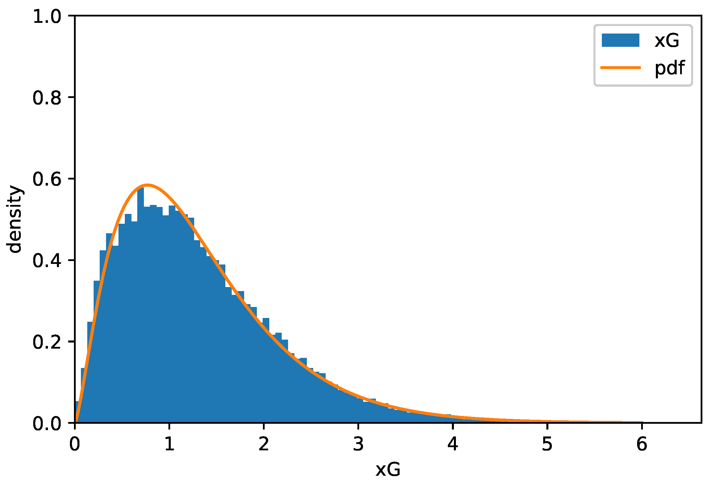
2014). In this work, we focus on Goals and expected Goals (xG) in data on N = 24,580 matches over 6 seasons between 2014–2015 and 2019–2020 from the Serie A, the Bundesliga, La Liga, the English Premier League, Ligue 1, and the Russian Premier League. Detail, such as the types and descriptions of the features, used in this section are provided in Table 5.
We use goals as an objective variable Y and xG as an explanatory variable X and assume Y | X P o ( exp ( β 0 + β 1 X ) ) as the true model. Thus, this Poisson regression model refers to the extent to which expected goals (xG) explains (true) goals. We assume that the true parameter β is obtained by the estimate from all N data.
As a diagnostic technique, we calculate a measure of goodness-of-fit to verify that the dataset follows a Poisson regression model. Table 6 shows estimates of ϕ and R M c F (McFadden 1974), where R M c F is the ratio of the log-likelihood estimate to the initial log-likelihood. ϕ = V [ Y | X ] / E [ Y | X ] is an overdispersion parameter. We may consider that overdispersion is not observed because ϕ = 1 equates to the standard Poisson regression model. The estimated value of β is ( 0.5225 , 0.5308 ) . Thus, we use this estimate as a true value. We assume X (xG) Γ ( k 1 , λ ) and obtain estimates of k 1 , λ as k 1 = 2.425 , λ = 1.851 (see Figure 1).
Expected goals (xG) is a performance metric used to represent the probability of a scoring opportunity that may result in a goal. xG is typically calculated from shot data. The measurer assigns a probability of scoring to a given shot and calculates the sum of the probabilities over a single game as xG. Observation error may occur in subjective evaluations. We can consider the situation that a high scorer happened to rate. Thus, we assume that X includes a stochastic error U given as
W = X + U .
Because W must be a positive value, we choose a positive error by U Γ ( k 2 , λ ) with k 2 = k 1 / 10 , k 1 / 3 , k 1 . We sample 1000 random samples from among all N samples to obtain the values of the estimates of β s. We repeat the estimations M C = 10,000 times to obtain the Monte Carlo mean of β s. The bias is calculated by the difference between the Monte Carlo mean and the true value.
Table 7 shows the estimated bias calculated by 10,000 simulations. The estimated bias of the corrected naive estimator is smaller than that of the naive estimator in all cases.
Next, we apply the naive and corrected naive estimators to financial data based on data collected in the FinAccess survey conducted in 2019, provided by Kenya National Bureau of Statistics (2019). In this study, we focus on the values labelled as finhealthscore and Normalized Household weights, with a sample size of N = 8669 . Details of the features used in this section, such as their types and descriptions, are provided in Table 8.
We use finhealthscore as an objective variable Y and normalized household weights as an explanatory variable X and assume Y | X P o ( exp ( β 0 + β 1 X ) ) as the true model. We further assume that the true parameter β is obtained by the estimate from all N data.
As a diagnostic technique, we calculate a measure of goodness-of-fit to verify that the dataset follows a Poisson regression model. Table 9 shows estimates of ϕ and R M c F (McFadden 1974). Overdispersion tends to occur to some extent in this Poisson regression model because the estimate of ϕ is greater than 1. The estimated value of β is ( 1.0442 , 0.1568 ) . As in the previous example, we regard the estimate as a true value. We assume X Γ ( k 1 , λ ) and obtain estimates of k 1 , λ as k 1 = 2.0746 , λ = 2.0746 (see Figure 2).
According to Kenya National Bureau of Statistics (2019), the data from the FinAccess survey were weighted and adjusted for non-responses to obtain a representative dataset at the national and county level. Thus, we may consider the situation that X exhibits a stochastic error U as
W = X + U .
We assume a positive error by U Γ ( k 2 , λ ) with k 2 = k 1 / 10 , k 1 / 3 , k 1 because the distribution of normalized household weights is positive. We sample random 1000 samples from among all N samples to obtain the values of the estimates of β s. We repeat the estimations over M C = 10,000 iterations to obtain the Monte Carlo mean of β s. The bias is calculated by the difference between the Monte Carlo mean and the true value.
Table 10 shows estimated bias calculated by 10,000 simulations. The estimated bias of the corrected naive estimator is smaller than that of the naive estimator in all cases.

7. Discussion

In this study, we have proposed a corrected naive estimator as a consistent estimator for a Poisson regression model with a measurement error. Although Kukush et al. (2004) showed that the naive estimator has an asymptotic bias, the authors did not provide a method to correct this bias. Therefore, we developed an approach to estimate a Poisson regression model with an error. In contrast, the authors of Kukush et al. (2004) also proposed a corrected score estimator and a structural quasi-score estimator for a Poisson regression model with an error. These estimators are score-based and consistent for unknown parameters. Hence, a generalization of these estimators should be considered in future research. In addition, the model considered in the present work is restricted in the univariate case. Extending the explanatory variable to the multivariate case also remains a challenge of note.

Author Contributions

K.W. mainly worked this study supported by the second named author. K.W.: Derivation of the formulae, Proof of propositions, Application to the specific problems, Conduct the simulation study, Real data analysis, Coding of the programs. T.K.: Basic idea, Theoretical advice of the proof, Advice at each step, Whole checking. All authors have read and agreed to the published version of the manuscript.

Funding

This research received no external funding.

Institutional Review Board Statement

Not applicable.

Informed Consent Statement

Not applicable.

Data Availability Statement

Data were obtained from https://understat.com/ and https://knbs.or.ke (accessed on 11 February 2023).

Acknowledgments

The authors thank to four anonymous referees for giving us valuable and insightful comments on the first draft. We missed future views of the draft and did not discuss drawbacks of our approach. Thanks to their sincere support for the draft, the revised version is now improved.

Conflicts of Interest

The authors declare no conflict of interest.

References

  1. Box, George Edward Pelham. 1963. The Effects of Errors in the Factor Levels and Experimental Design. Technometrics 5: 247–62. [Google Scholar] [CrossRef]
  2. Burr, Deborah. 1988. On Errors-in-Variables in Binary Regression-Berkson Case. Journal of the American Statistical Association 83: 739–43. [Google Scholar]
  3. Geary, ROBERT C. 1953. Non-Linear Functional Relationship between Two Variables When One Variable is Controlled. Journal of the American Statistical Association 48: 94–103. [Google Scholar] [CrossRef]
  4. Guo, Jie Q., and Tong Li. 2002. Poisson regression models with errors-in-variables:implication and treatment. Journal of Statistical Planning and Inference 104: 391–401. [Google Scholar] [CrossRef]
  5. Huwang, Longcheen, and YH Steve Huang. 2000. On error-in-variables in polynomial regression-Berkson case. Statistica Sinica 10: 923–36. [Google Scholar]
  6. Jiang, Fei, and Yanyuan Ma. 2020. Poisson Regression with Error Corrupted High Dimensional Features. Statistica Sinica 32: 2023–46. [Google Scholar] [CrossRef]
  7. Kenya National Bureau of Statistics (KNBS). 2019. Available online: https://knbs.or.ke (accessed on 11 February 2023).
  8. Kukush, Alexander, and Hans Schneeweiss. 2000. A Comparison of Asymptotic Covariance Matrices of Adjusted Least Squares and Structural Least Squares in Error Ridden Polynomial Regression. Sonderforschungsbereich 386: Paper 218. [Google Scholar] [CrossRef]
  9. Kukush, Alexander, Hans Schneeweis, and Roland Wolf. 2004. Three Estimators for the Poisson Regression Model with Measurement Errors. Statistical Papers 45: 351–68. [Google Scholar] [CrossRef] [Green Version]
  10. McFadden, Daniel. 1974. Conditional logit analysis of qualitative choice behavior. Computations in Statistics-Theory and Methods 47: 105–42. [Google Scholar]
  11. Nakamura, Tsuyoshi. 1990. Corrected score function for errors-in-variables models: Methodology and application to generalized linear models. Biometrika 77: 127–37. [Google Scholar] [CrossRef]
  12. Shklyar, Schneeweiss, and Hans Schneeweiss. 2005. A comparison of asymptotic covariance matrices of three consistent estimators in the Poisson regression model with measurement errors. Journal of Multivariate Analysis 94: 250–70. [Google Scholar] [CrossRef] [Green Version]
  13. Understat. 2014. Available online: https://understat.com/ (accessed on 11 February 2023).
Figure 1. Distribution of xG.
Jrfm 16 00186 g001
Figure 2. Distribution of normalized household weights.
Jrfm 16 00186 g002
Table 1. Estimated bias of a Gamma distribution with a Normal error.
Asy.Bias β ^ 0 BIAS ( β ^ 0 ) ^ Asy.Bias β ^ 1 BIAS ( β ^ 1 ) ^
σ 2 = 0.05 Naive0.011110.01139−0.005993−0.007199
CN00.0000353200.0002603
σ 2 = 0.5 Naive0.099120.1025−0.05297−0.05582
CN00.00781700.0007142
σ 2 = 2 Naive0.27570.2774−0.1454−0.1472
CN0−0.00949300.002736
Table 2. Estimated MSE of a Gamma distribution with a normal error.
Asy.MSE β ^ 0 MSE ( β ^ 0 ) ^ Asy.MSE β ^ 1 MSE ( β ^ 1 ) ^
σ 2 = 0.05 Naive0.00012350.0030030.000035920.0004536
CN00.00292000.0004254
σ 2 = 0.5 Naive0.0098240.013620.0028060.003508
CN00.00380600.0006354
σ 2 = 2 Naive0.076000.081240.021150.02214
CN00.0102100.002160
Table 3. Estimated bias of a Gamma distribution with a Gamma error.
Asy.Bias β ^ 0 BIAS ( β ^ 0 ) ^ Asy.Bias β ^ 1 BIAS ( β ^ 1 ) ^
k 2 = 0.072 Naive−0.002634−0.005415−0.007887−0.008874
CN0−0.000663600.0002777
k 2 = 0.72 Naive−0.02090−0.01725−0.06378−0.06475
CN0-0.00029630−0.003184
k 2 = 2.88 Naive−0.04953−0.05439−0.1558−0.1569
CN00.0029540−0.003224
Table 4. Estimated MSE of a Gamma distribution with a Gamma error.
Asy.MSE β ^ 0 MSE ( β ^ 0 ) ^ Asy.MSE β ^ 1 MSE ( β ^ 1 ) ^
k 2 = 0.072 Naive0.085330.0031090.0000069400.0005384
CN00.00307400.0004743
k 2 = 0.72 Naive0.055800.0053200.00043680.004894
CN00.00445700.0008818
k 2 = 2.88 Naive0.020800.011470.0024530.02553
CN00.00740100.001963
Table 5. Details of the variables.
FeaturesTypeDescription
Goalscountingnumber of goals scored in the match
xGcontinuousperformance metric used to evaluate football team and player performance
Table 6. Estimates of ϕ and R M c F .
ϕ ^ R McF ^
0.89070.1589
Table 7. Estimated bias and asymptotic bias in football data.
Asy.Bias β ^ 0 BIAS ( β ^ 0 ) ^ Asy.Bias β ^ 1 BIAS ( β ^ 1 ) ^
k 2 = k 1 / 10 Naive−0.01148−0.01337−0.03534−0.03471
CN0−0.00180400.0006200
k 2 = k 1 / 3 Naive−0.03263−0.02383−0.1020−0.1067
CN00.0081760−0.005575
k 2 = k 1 Naive−0.06889−0.04692−0.2210−0.2291
CN00.018710-0.01215
Table 8. Details of the variables.
FeaturesTypeDescription
finhealthscorecountingScore of financial health for households
Normalized Household weightscontinuousWeighted and normalized households
Table 9. Estimates of ϕ and R M c F .
ϕ ^ R McF ^
1.43600.4478
Table 10. Estimated bias and asymptotic bias in financial data.
Asy.Bias β ^ 0 BIAS ( β ^ 0 ) ^ Asy.Bias β ^ 1 BIAS ( β ^ 1 ) ^
k 2 = k 1 / 10 Naive−0.0005704−0.002225−0.01327−0.01207
CN0−0.00162800.001275
k 2 = k 1 / 3 Naive−0.001581−0.004088−0.03694−0.03522
CN0-0.00240400.002119
k 2 = k 1 Naive−0.003204−0.008314−0.07534−0.07283
CN0−0.00474400.004338
Disclaimer/Publisher’s Note: The statements, opinions and data contained in all publications are solely those of the individual author(s) and contributor(s) and not of MDPI and/or the editor(s). MDPI and/or the editor(s) disclaim responsibility for any injury to people or property resulting from any ideas, methods, instructions or products referred to in the content.

