
Balance of Risks and the Anchoring of Consumer Expectations
Department of Economics, University of Notre Dame, Notre Dame, IN 46556, USA
J. Risk Financial Manag. 2023, 16(2), 79; https://doi.org/10.3390/jrfm16020079
Submission received: 30 December 2022
/
Revised: 16 January 2023
/
Accepted: 21 January 2023
/
Published: 28 January 2023
(This article belongs to the Special Issue Central Banking and Financial Stability)
Abstract
:This paper shows that expected inflation risks pose threats to the anchoring of expectations. I propose a new method for fitting subjective probability distributions to density forecasts that allows for asymmetric beliefs over inflation outcomes. Using data from the Federal Reserve Bank of New York’s Survey of Consumer Expectations, I show that medium run expectations move in the direction of perceived short run risks. A diffusion index of consumers’ perceived balance of risks to inflation shows that high short run inflation expectations coincide with the balance of medium risks being weighted to the upside.
Keywords:
inflation; risks; consumer expectations; balance of risks; subjective distributions; anchoringJEL Classification:
E31; D83; D841. Introduction
Monetary policymakers have as a critical goal the anchoring of inflation expectations. Theory predicts that stable expectations lead to stable inflation (Orphanides and Williams 2007). Price stability may in turn facilitate financial stability. When inflation is low, market participants may interpret an asset’s price as a reliable metric of its real economic value. When inflation is high, it becomes more difficult to disentangle market-driven price fluctuations from inflationary fluctuations. Low and stable inflation can also provide monetary policymakers with the flexibility to smooth business cycle and financial shocks (Bernanke 2006). Central banks accordingly devote considerable attention to monitoring expectations and the extent to which they are anchored (or de-anchored). Research has defined well-anchored expectations as close to the central bank’s inflation target, unresponsive to short-term fluctuations, and expressing minimal subjective uncertainty (Kumar et al. 2015). Recent work has also considered the cross-sectional skewness of expectations as an indicator of de-anchoring. Reis (2021) shows that a thickening of the right tail of the cross-sectional inflation distribution is among the first sign of upside de-anchoring. Natoli and Sigalotti (2018) shows that the negative tail of the options-implied short run inflation expectation distribution is associated with lower long run beliefs.
This paper considers how the inflation risks that consumers expect contribute to the (de-)anchoring of expectations. Monetary policymakers often speak in terms of risk to the inflation outlook and particularly in terms of unbalanced risk.1 In a 2020 speech, former Vice Chair of the Federal Reserve Richard Clarida said of the expectations of FOMC participants, “there is no presumption that the subjective distributions—or, for that matter, observed empirical distributions—for [inflation] are symmetric.” This highlighting of the potential for asymmetry in subjective distributions accompanies the addition of historical values of the diffusion index of participants’ inflation risk weightings to the Summary of Economic Projections (SEP).2 A forecaster’s “balance of risks” or “risk weighting” indicates the direction of risks (high inflation v. low inflation or deflation) that the forecaster believes is more likely. The risks to inflation itself vary over time; understanding whether consumers anticipate inflationary or deflationary risks indicates the direction in which expectations may become de-anchored. In its communication with the public, the Federal Reserve projects that they view price stability and expectations monitoring with an eye towards the direction of risks. Their goal is to keep tail risks to inflation from becoming realized in inflation itself.3 Preventing perceived short run tail risks from moving into long run expectations is a complementary goal.
The availability of density inflation forecasts allows us to consider how the expected risks implied by an individual’s subjective probability distribution over inflation signal threats to anchoring. Using data from the Federal Reserve Bank of New York’s Survey of Consumer Expectations (SCE) from 2013 through the end of 2021, this paper examines empirically consumers’ perceived inflation tail risk. I first introduce a method of fitting subjective distributions that incorporates a respondent’s point forecast as the mode of their subjective distribution and allows for asymmetry in these distributions. The resultant distributions have similar interpretations to the SEP projections and an assessed balance of risks. The central tendency of the distribution is close to the most likely perceived outcome, while the skewness gives the risk weighting around this projection. A positively skewed distribution reveals a perceived risk that is weighted to the upside; the bulk of the distribution is located around a low level of inflation with the tail—or perceived to be rare—outcome located at higher values of inflation. This novel method for fitting a distribution to probabilistic forecasts allows for asymmetry in subjective inflation distributions.4
Do anticipated risks to inflation pose a threat to the anchoring of longer run expectations? Kumar et al. (2015) posits that anchored long run expectations should not be predictable given short run expectations. I extend this framework for anchored expectations to argue that anchored long run expectations should be unpredictable given the risks implied by consumers’ subjective probability distribution over short run inflation. I find that upside (downside) tail risk in the subjective distribution of year-ahead inflation moves the central tendency of the expected three year-ahead distribution up (down). This implies that consumers believe inflation will move over the medium term in the direction of their perceived risk, suggesting that monetary policymakers should consider monitoring tail risks in expectations. Structuring communication to manage these risks and prevent de-anchoring may further promote financial stability.
To track the predominant direction of perceived risks to inflation over time, I construct a diffusion index of consumers’ perceived balance of risks to near-term and medium-term inflation paralleling the SEP diffusion index for FOMC participants. This index subtracts the share of consumers with negatively-skewed distributions from the share of positively-skewed distributions. In a given period, the index will increase as more consumers perceive inflationary risk relative to their modal projection and decrease as more consumers perceive disinflationary or deflationary risk. In 2021, the value of this index for medium-run inflation and aggregate level of short-run expectations rose to their highest levels in survey history.
My paper fits most closely with the literature on risks in inflation expectations. These include (Andrade et al. 2012, 2014) that derive measures of inflation risk for professional forecasters in the U.S. and Eurozone, respectively. García and Manzanares (2007) fit a skewed-normal distribution to probabilistic forecasts from the U.S. Survey of Professional Forecasters to allow for asymmetry in these forecasts. Ruge-Murcia (2003) considers a central banker’s utility under deviations from the inflation target, with the potential for asymmetric preferences over the direction of risks. Killian and Manganelli (2008) model a central banker as a risk manager who must manage the risks of inflation falling outside the range of a targeting zone, with the potential for asymmetric risk aversion in upside and downside risks. Galati et al. (2021) show that long-run inflation expectations of Dutch households are poorly anchored, largely due to household’s placing large probability on inflation outcomes above the central bank’s target. Using financial market data, Fleckenstein et al. (2017) and Apergis and Apergis (2021) use U.S. inflation swaps and options to measure the markets perceived deflation risk and inflation expectations, respectively. Gimeno and Ibanez (2018) uses European options to study expected tail risks to Euro area inflation. Adams et al. (2021) uses quantile regression to measure macroeconomic risks around consensus forecasts from the Survey of Professional Forecasters. These last two papers focus—as this paper does—on the direction of risks to the macroeconomic outlook.
I also contribute to the literature on fitting subjective distributions to probabilistic forecasts. D’Amico and Orphanides (2008) fits a normal distribution to density forecasts. Engelberg et al. (2009) proposes a method fitting triangular distribution to histograms where the respondent fills one or two bins and a parametric generalized beta distribution when the respondent fills three or more bins. The SCE uses this same method with the modification that they assume a uniform distribution for respondents filling a single bin (Armantier et al. 2016). I modify the (Engelberg et al. 2009) method by pinning the mode of a consumer’s subjective probability distribution to her point forecast.
Another set of papers considers the effect of inflation and inflation risk on financial markets and financial market participants. Vukovic et al. (2022) explores how inflation affects portfolio selection using quantile regression. Chaudary and Marrow (2022) and Boon et al. (2020) explore how inflation expectations and inflation risks, respectively, are priced into the stock market.
The paper proceeds as follows: Section 2 describes the data as well as my proposed method for fitting subjective distributions. This method incorporated asymmetry into subjective inflation distributions. Accordingly, in Section 3, I argue that this method provides a useful measure for aggregate expectations in this dataset and shows how asymmetry is incorporated into these distributions. Section 4 discusses how perceived tail risks in short run inflation affect their medium run expectations. This section shows that, ceteris paribus, an individual’s medium run expectations are predictable from the direction of the risks they anticipate to short run inflation. Section 5 discusses the diffusion index for SCE respondents as an aggregate measure of perceived inflation risk and shows that perceptions of risks in the medium term increase with expectations of short run inflation. Section 6 situates the paper alongside similar work and concludes with a discussion of the recent history of inflation expectations.
2. Data
I use monthly inflation expectations data from from the Federal Reserve Bank of New York’s Survey of Consumer Expectations. This survey is a representative rotating panel of American households. These households remain in the survey for up to 12 months. The sample period includes data from June 2013 to December 2021, the last date for which microdata are publicly available. This yields 130,250 observations across 18,549 households. Household heads provide their inflation expectations in two formats, first as a point estimate and then as probabilities that inflation may fall in a set of ranges. They are first asked:
What do you expect the rate of [inflation/deflation] to be over the next 12 months?5 Please give your best guess.
Respondents provide this answer as a percentage. Many consumers respond with particularly high values of inflation. For example, 13% of respondents provide a forecast of 10% or higher. As such, the Federal Reserve Bank of New York elicits density forecasts of inflation and calculates the mean implied by a probability distribution fitted to the resulting histogram. The density forecast question asks consumers to consider several possible outcomes for inflation.
Now, we would like you to think about the different things that may happen to inflation over the next 12 months. We realize that this question may take a little more effort.
In your view, what would you say is the percent chance that, over the next 12 months...
The respondent is then presented with a set of ranges for the rate of inflation or deflation, where deflation is defined for them as the opposite of inflation. The ranges are a rate of inflation or higher, between and , between and , between and , between and , and the same set of bins for the rate of deflation. The questions eliciting point estimates and subjective distributions are repeated for the agent’s expectations of inflation over the 12 month period from 24 months from the survey period to 36 months after the survey period. I refer to the expectations over the next 12 months as short run inflation expectations and expectations over the period from 24 to 36 months from the survey date as medium run inflation expectations.
Considered together, the point and density forecasts can provide information about the shape of an individual’s subjective probability distribution. Using the point estimate rather than fitting a subjective distribution without it allows for the expression of additional heterogeneity (across and within) forecasters that provide identical histogram forecasts. Define a unique histogram forecast as a set of answers for each of the bins for either short run or medium run inflation. A unique forecast refers to a given unique histogram forecast coupled with a point forecast. Across all household-date observations in the survey, there are roughly 1.5 times as many unique forecasts as unique histogram forecasts.6 Households will repeat the same unique histogram forecast multiple times with different point estimates. Among these forecasts repeated by the same household, only roughly include the same point estimate across all repetitions. This means that a given household’s expectations may be moving even as the histogram forecast remains stable.
The data suggest that households make point estimates consistent with the modes of their subjective distribution. Define a modal forecast as a point estimate that falls in the bin in which a household places maximum probability.7 The majority of consumers give point forecasts consistent with the modal definition— of short run forecasts and of medium run ahead forecasts are modal forecasts. This contrasts with of short run and medium run forecasts that fall in the same bin as the mean forecast calculated by the SCE.
I fit subjective probability distributions closely paralleling the method of (Engelberg et al. 2009). They construct subjective distributions by fitting isoceles triangles to the histograms of respondents placing positive probability in one or two bins and generalized beta distributions to the histograms of respondents filling three or more bins. My method pins the mode of the distribution to the consumer’s point estimate and fits a scalene triangle to one- and two-bin forecasts and a generalized beta with a fixed mode to forecasts with positive probability in three or more bins. This method is described in detail in Appendix A. The method has two main advantages over (Engelberg et al. 2009). First, in these data, point forecasts are modal forecasts and this method reflects that. The second advantage is that this method allows for asymmetry in subjective probability distributions over inflation. This enables the expression of unbalanced expected risks to inflation or expected risks in one direction and not the other.
Denote the implied medians of the short run and medium run distributions as and , respectively, and the means as and . I use the interquartile range, as a measure of the second moment and solve for (Bowley 1920)’s measure of skewness for each individual distribution:
where denotes the 75th percentile and the other percentiles are similarly notated. The skewness of the subjective distribution also represents a consumer’s perceived balance of risks. If the distribution is skewed to the right, the perceived tail risk is at levels of inflation above the inflation outcome that the consumer has deemed most likely. This means that the balance of risks to inflation is weighted to the upside. When the distribution is negatively skewed, the balance of risks is weighted to the downside; that is, the expected tail outcome is below the consumer’s most likely inflation outcome.
I quantify tail risks in either direction by defining the left and right tails as the difference between percentiles:
These give measures of how far the extremes of the distribution go. The left tail tells us how far beyond the 25th percentile the distribution extends to downside outcomes. The right tail captures the range of upside outcomes beyond the 75th percentile. Measures of inflation-at-risk or expected inflation-at-risk, such as those discussed in (Andrade et al. 2012 and López-Salido and Loria 2022), measure risk by value of the 25th or 75th percentile. The tails as I have defined them give a sense of how far a consumer thinks inflation can go in either direction conditional on reaching an already high or low level. The right (left) tail will increase in length as rare perceived outcomes are weighted more to the upside (downside). A tail will decrease in length if the mode of the distribution is close to the relevant bound of the support of the consumer’s subjective distribution. An example helps illustrate what these tails measure. Consider a consumer whose subjective probability distribution over inflation has a 75th percentile at 5%. If the 95th percentile of this distribution is at 6%, the tail length will be 1 percentage point. If the consumer had a subjective probability distribution with the same 75th percentile and a 95th percentile at 7%, the tail length would increase to 2 percentage points. The consumer with the longer tail length places positive probability on more extreme outcomes. I use the tails rather than the 5th and 95th percentiles themselves because these percentiles are highly correlated with the median of the distribution. The transformation reduces the multicollinearity problem and provides information about anticipated extreme outcomes independent of the location of the distribution.
Table 1 provides summary statistics for these values over the sample period. The survey-weighted average implied mean throughout the sample for both short run and medium run is roughly 4.2 and 4.0, respectively. The average IQR is roughly 5.5 and the the average left and right tails roughly 3.0 and 2.8, respectively. These numbers are large compared to a series that is targeted to 2% for the entirety of the sample period. We should keep these magnitudes in mind when considering how components of the short run distribution will impact medium run-expectations. The average distribution is symmetric, indicating an approximate balance of consumers having positively- and negatively-skewed distributions. However, this balance changes from period to period, as will be discussed in Section 5.
3. A New Measure of Expected Inflation
I propose measuring aggregate consumer expectations with the subjective fit using the method described briefly in Section 2 and in detail in Appendix A.8
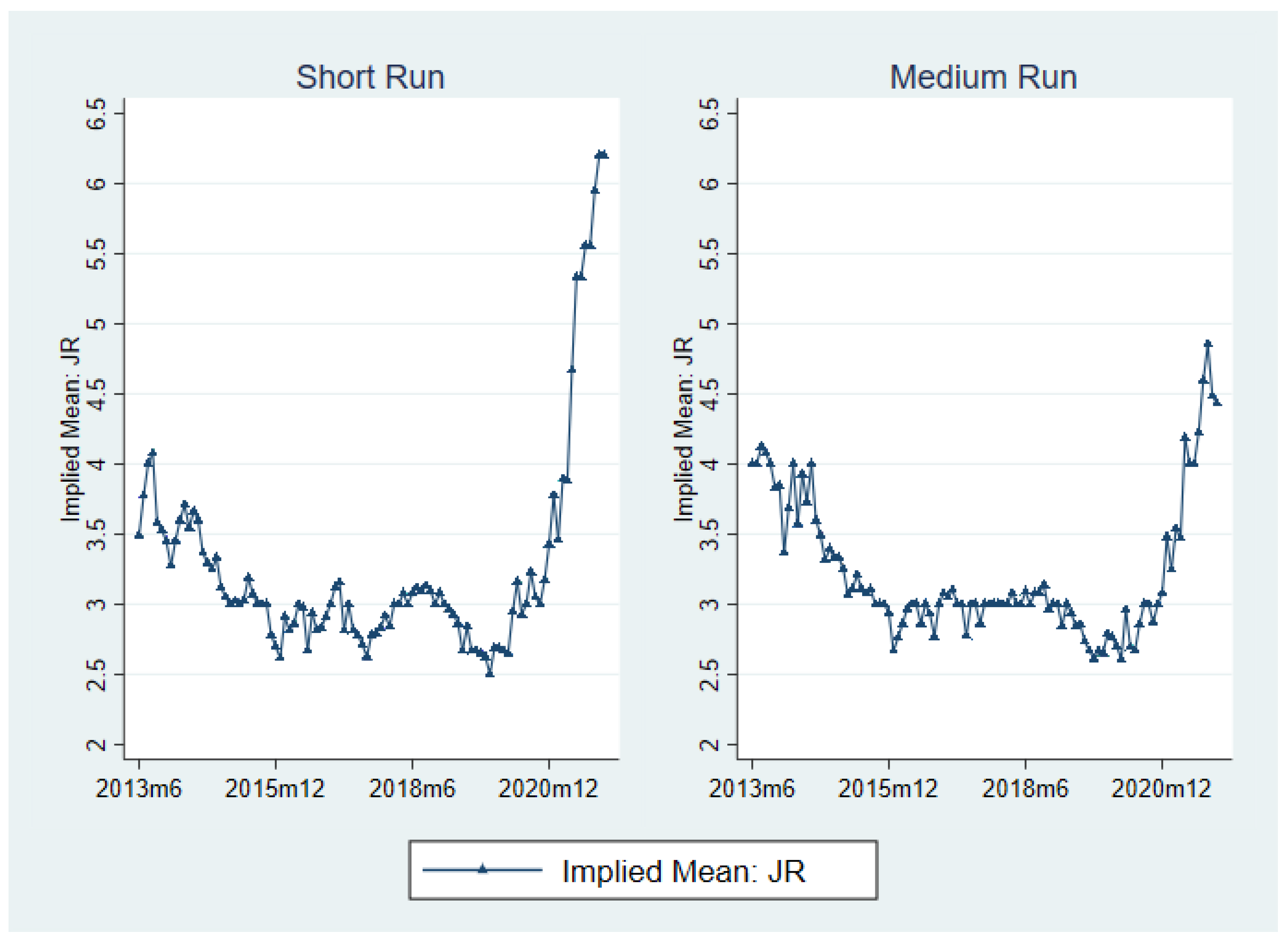
Figure 1 plots these medians over time for short run and medium run expectations. Both series trend downwards for the first two years of the survey, potentially reflecting growing public understanding of the Federal Reserve’s inflation target. Towards the end of the sample, into the COVID period, the medians increase, reflecting the public perception that the pandemic would increase inflation (Binder 2020). The two series increase to similar levels in 2020. In 2021, aggregate expected year-ahead inflation exceeds 6%. The aggregate value of three-year ahead inflation stays below 5%.
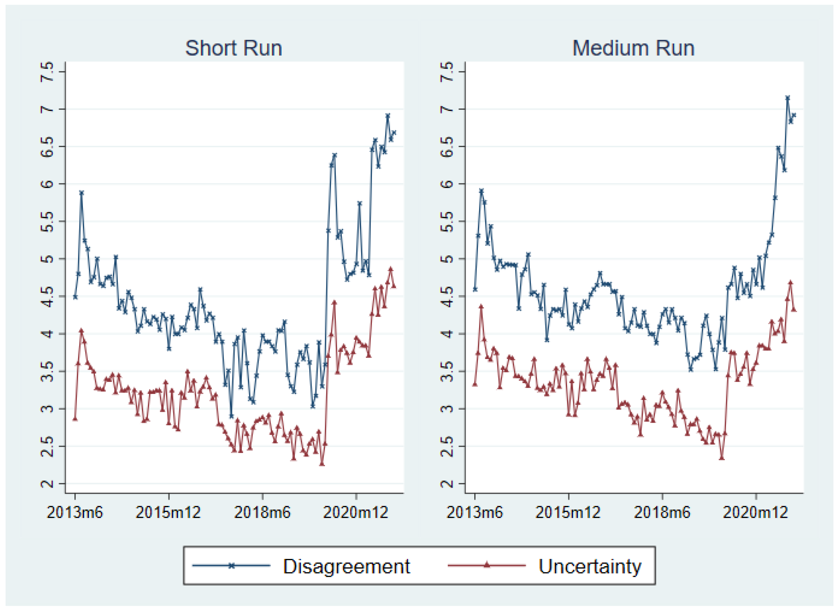
Figure 2 plots the measures of cross-sectional disagreement and subjective uncertainty for short run and medium run expectations. The dispersion is calculated as the cross-sectional interquartile range of inflation expectations in a period. An individual’s subjective uncertainty is defined as the interquartile range of her subjective distribution over inflation outcomes. The time series measure of uncertainty in the figure is the median of these IQRs in a given period. Uncertainty is generally larger than disagreement, supporting the empirical findings of (D’Amico and Orphanides 2008; Rich and Tracy 2021; Rich et al. 2012 and Coibion et al. 2021) that disagreement is an imperfect proxy for subjective uncertainty. Uncertainty and disagreement both decline over the sample period until 2020. In March 2020, both increase and remain high, a potential sign of de-anchoring. In 2021, disagreement and uncertainty increased even more.
Comparison to the SCE Measure
The Survey of Consumer Expectations currently publishes a similar measure of aggregate expectations. They use the means implied from the subjective distributions fit using the method of (Engelberg et al. 2009) as described in (Armantier et al. 2016). This method assumes symmetric distributions for respondents with histogram forecasts filling one or two bins. In comparison, the method I propose allows for asymmetry in subjective distributions. This section provides a visual example of how my method incorporates asymmetry into these distributions. As roughly 30% of respondents fill one or two bins, the assumption of symmetry will impact a large number of observations and, consequently, any aggregate measure derived from these distributions.
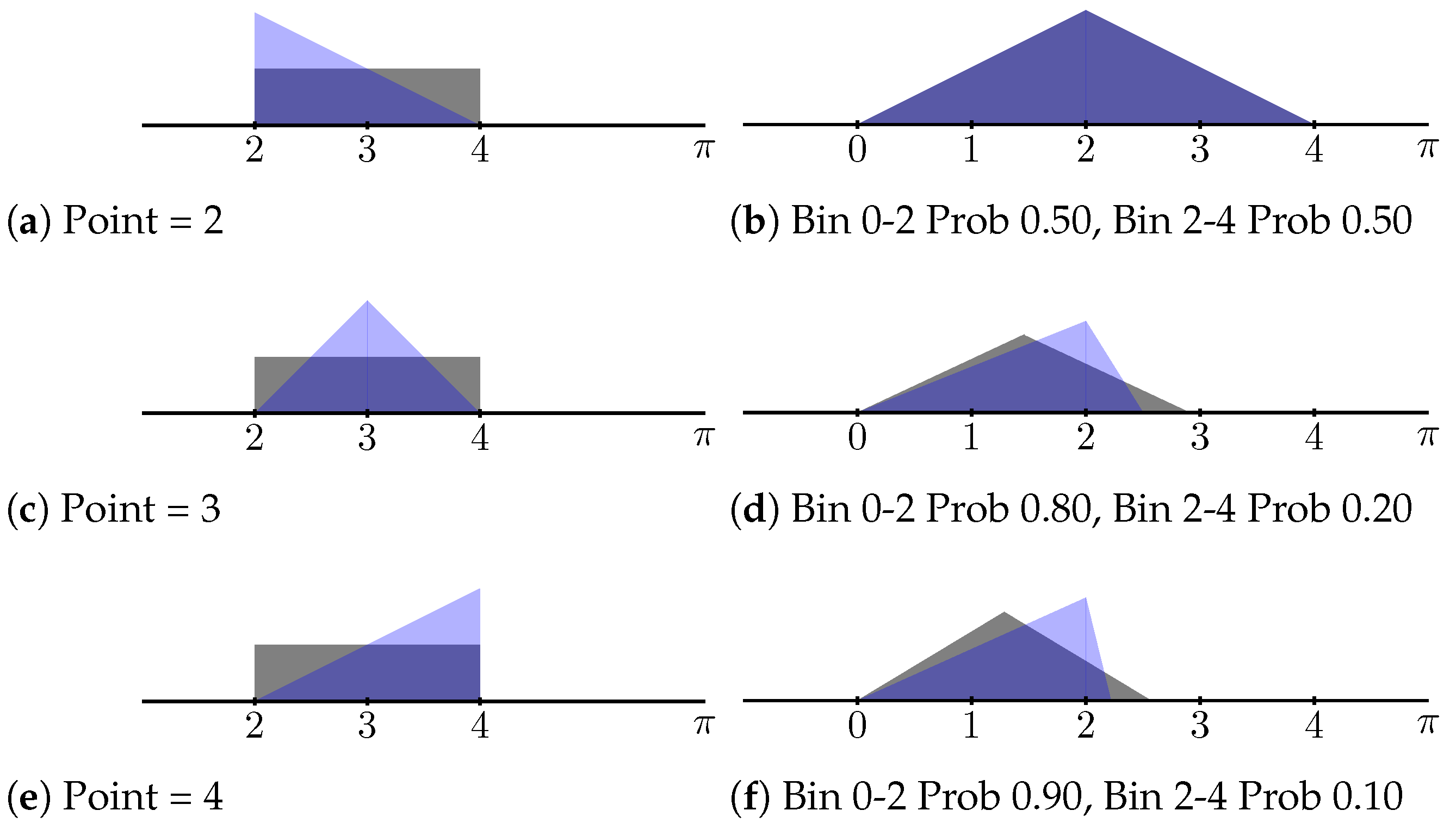
Figure 3 shows the difference in the subjective probability distributions generated by the different methods. The mode assumption allows for heterogeneity in implied central tendency and uncertainty across households that place all probability in a single bin. It also moves the mean of the subjective distribution closer to the respondent’s point estimate, which is particularly useful if a respondent’s point forecast is more likely to fall to one side of the interval than the other. Consider, for example, the bin placing inflation between and . Of the 4523 respondents who assign probability only to this bin, 1372 also report a point estimate of at or below 2%. Only 844 report a point estimate at or above 4%. Figure 3a,c show the fitted subjective probability distribution for these two cases. Under my proposed fitting method, these two forecasts differ both in implied mean and in the direction of the predominant tail risk. There is a meaningful difference in the subjective distributions of a consumer who thinks that inflation will be 2% or higher (up to 4%) and a consumer who thinks that inflation will be 4% or lower (down to 2%).
The second column demonstrates how my method introduces asymmetry in two-bin forecasts. It compares forecasts with positive probability in the bins to and to and report a point forecast of 2% inflation. In the case where the respondent assigns equal probability to the two bins, depicted in Figure 3d, the point estimate falls at the exact midpoint of the interval and the two methods produce the same distribution. As the probability in the rightmost bin decreases the distribution fitted by the SCE and (Engelberg et al. 2009) remains an isoceles triangle with the peak moving away from the point estimate at 2. In contrast, my method keeps the peak of the triangular distribution at 2 and moves the right endpoint to form a scalene triangle. This is shown in Figure 3e,f. This method concentrates subjective density near the point estimate, with implications for measures of uncertainty, asymmetry, and tail risk.
4. Short Run Risks and Medium Run Expectations
Well-anchored long-run expectations should remain stable and insensitive to movements in short run expectations. While short run expectations may move with macroeconomic shocks, well-anchored long-run expectations should remain firmly fixed by the central bank’s target. I propose that well-anchored longer-run expectations should be uncorrelated with the perceived balance of risks (given by the skewness of a respondent’s subjective distribution) or perceived short run risks (given by the tails of the short run distribution described in Section 3). If long run expectations always return to the inflation target, they should not drift towards the tails of the short run distribution even if one of these tails represents the predominant direction of risks in a consumer’s mind.
Kumar et al. (2015) refers to long-run expectations as increasingly anchored if they are not influenced by fluctuations in short run beliefs. They propose regressing long-run forecasts on short run forecasts. If expectations are well-anchored, the coefficient on short run expectations should be equal to zero. I extend this regression to include measures of anticipated risks and their predominant direction. The skewness represents the balance of risks or the direction of risks to inflation the consumer expects. The left and right tails provide measures of the extremity of the downside and upside risk, respectively, the consumer anticipates.
I first estimate the following specification, regressing the implied median of the medium run distribution, , on the implied mean of the short run distribution, , as well as the skewness, and the interquartile range (IQR) of the short run distribution:
The regression includes fixed effects for respondent and date. The date fixed effect control for unobservables such as macroeconomic conditions that may affect both short run and medium run expectations. For example, following an uncertainty shock, inflation uncertainty () may increase. Consumers may also anticipate increased likelihood of recession, affecting (Alessandri and Mumtaz 2019). Controlling for time fixed effects focuses on variation in expectations across consumers. Including individual effects controls for potential systematic patterns in a consumer’s responses throughout her survey tenure. Research suggests that household inflation expectations vary systematically, often with features of the household that do not change over time (D’Acunto et al. 2022); fixed effects can control for these factors. A Hausman test shows that fixed effects are preferred to random effects.
The coefficients appear in Table 2. The table also presents the p-value of the Hausman test. If expectations are well anchored, we would expect all of the coefficients to be equal to 0; all, however, are statistically different from 0. The coefficient on indicates that those with higher short run inflation expectations also have higher medium run inflation expectations. The positive coefficient on skewness means that the central tendency of a respondent’s medium run distribution moves in the same direction as her perceived balance of short run risks.
I estimate again extend this analysis adding to the regression measures of the left and right tails:
The short run median, both tails, and the interquartile range all have statistically significant coefficients, meaning that fluctuations in the subjective probability distribution influence longer-run expected inflation. The coefficient on skewness is still positive but no longer statistically significant; as I include measures for both tails, the asymmetry of the distributions is likely captured by the varying tail lengths. Increased length in the tails draws in the direction of the tail. Increased length in a tail of the distribution means that a respondent thinks that a wider range of extreme outcomes in that direction are possible. The coefficient on the right tail means that, as the tail of the short run distribution extends an additional percentage point to the right, all else being equal, the median of the medium run distribution increases by 0.13 percentage points. This means that consumers who anticipate greater inflationary risks to short run inflation also anticipate higher inflation in the longer term. As the left tail extends one percentage point further into outcomes that are low compared to the rest of the respondent’s distribution, the median of the medium run distribution decreases by 0.07 percentage points. As perceived short run risks in inflation expectations can move longer run expectations, they are a relevant consideration for the anchoring of longer run expectations.
5. Short Run Expectations and Medium Run Risks
The previous section argued that perceived risks to short run inflation can move longer run expectations. This section considers the relationship between short run expectations and longer-run risks. When consumers expect higher inflation in the short run, do they also anticipate more inflationary risks in the medium run? Do the long run distributions remain centered around the central bank’s targeting, indicating well-anchored expectations? To explore this question, I first propose a diffusion index of the risk weightings of consumers in the Survey of Consumer Expectations. This parallels the public reports of SEP whose goal is to indicate the direction of risks anticipated by the majority of FOMC members. The diffusion index I propose shows the direction of risks perceived by the majority of consumers in the SCE in a given period.
The skewness calculated in Equation (1) can be interpreted in terms of the risk weighting FOMC participants report about their inflation projections. Positively-skewed distributions correspond with a belief that risks are weighted to the upside; negatively-skewed distributions indicate a belief that risks are weighted to the downside. The index over the balance of risks is then given by:
where the shares are survey-weighted. This number will increase as the share of positively skewed increases and will decrease as the share of negatively skewed distributions increases. It is bounded between [−1 and 1], with −1 meaning all respondents expect predominantly downside risk and 1 meaning all respondents weight risk to the upside. Positive values mean relatively more respondents anticipate inflationary risk while negative values mean more respondents anticipate disinflation around their modal forecast. I derive this index for both short run and medium run expectations: , .
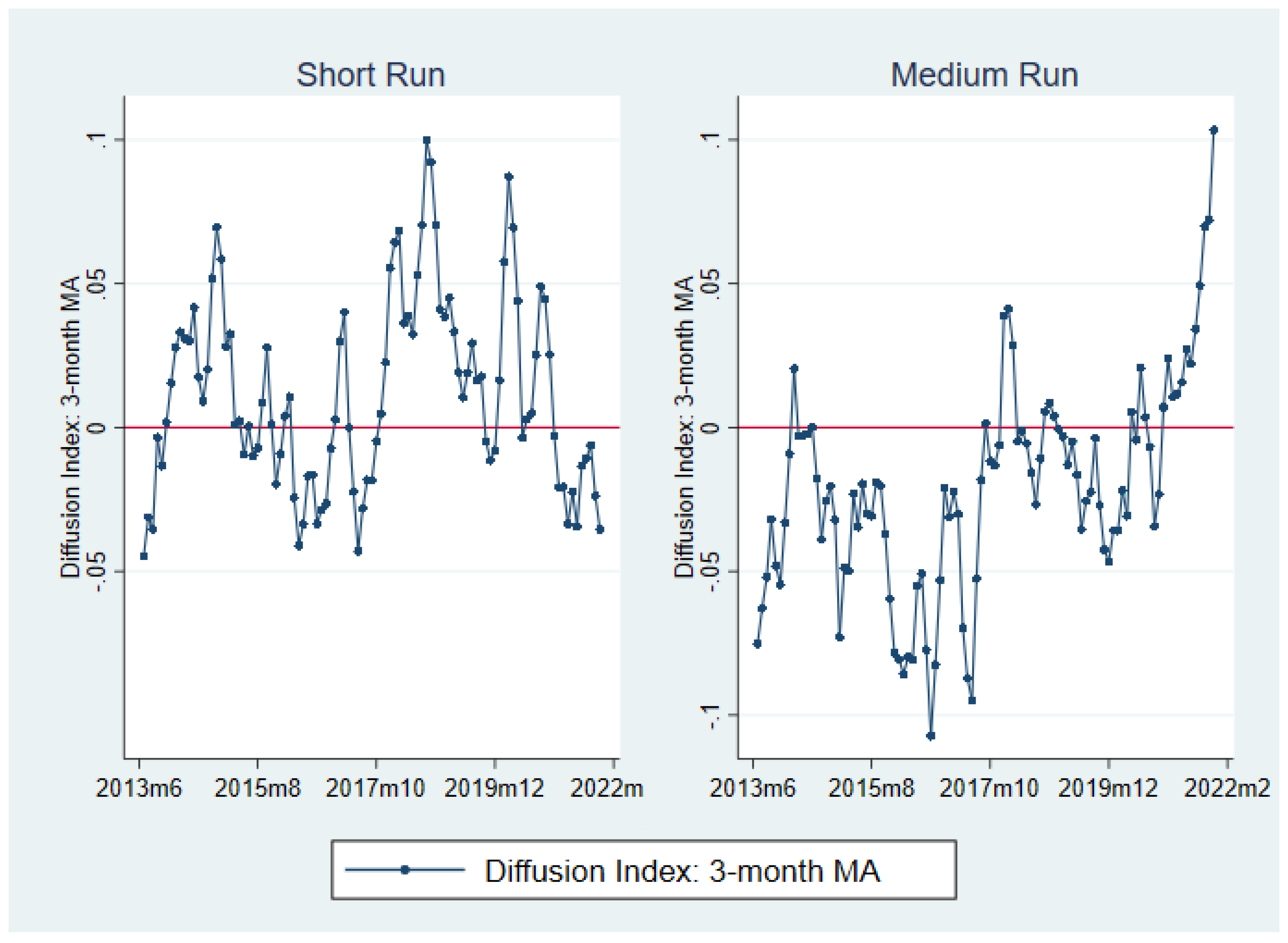
Figure 4 shows the three-month moving averages of these two series plotted over time. In addition, the x-axis is highlighted as a diffusion index of 0 indicates a that the survey is evenly weighted between those with positively- and negatively-skewed distributions. Throughout the sample period, the short run index shows that the majority of respondents expect predominantly upside risk. Conversely, the medium run series indicates that more respondents expect downside risk. The series have relatively low correlation, 0.29, indicating that they do not always move together. For example, in the early COVID period, when aggregate short run risk perceptions swung to the upside, medium run risk perceptions moved to the downside. Consumers may have anticipated higher inflation in response to the pandemic as (Binder 2020) finds, but expected short run inflation to revert back to long run mean levels, which would indicate anchoring. In 2021, the pattern reversed. The majority of consumer expected short run risks to be weighted to the downside and medium run risks to be weighted to the upside.
By the end of 2021, the diffusion index for medium run inflation was at its highest level in survey history, with a difference in the share expecting upside risk and the share expecting downside risk equal to 10 percentage points. At this time, both the medium-run and short-run expectations were increasing. For well-anchored inflation expectations, a change in the central tendency of aggregate short run expectations should not generate perceived risk in medium run expectations. Consumers might expect, however, that shorter run outcomes may bring with them factors that may affect medium run inflation. In this case, changes in the aggregate short run expectation will move the aggregate risk perception. I test this with the following regression:
The coefficient of interest is . I control for the aggregate medium run expectation as higher or lower medium run inflation may be associated with a change in the associated risks. I also control for the short run diffusion index as there may be a correlation between the aggregate short run and medium run risk weightings. The results appear in Table 3. Notably, a one percentage point increase in the median medium run expectation increases the medium run diffusion index by 6 percentage points, increasing the share of respondents who expect that the risks to medium run inflation are weighted to the upside. This means that changes in expectations are absorbed into concerns about tail outcomes in longer run inflation.
6. Discussion
This paper extends the work of (Engelberg et al. 2009) in proposing a new method of fitting subjective probability distributions to histogram forecasts. This method is an improvement as it allows for the expression of unbalanced risk in consumer’s inflation expectations. I further build on the work of (Kumar et al. 2015) in using components of individual consumers’ expected distributions over short run inflation.
This paper contributes to the set of papers considering inflation risks in particular. While many of these papers measure aggregate risks using market perceptions implied by derivative contracts on inflation—(Fleckenstein et al. 2017; Apergis and Apergis 2021; Gimeno and Ibanez 2018)—I use survey data on inflation expectations. (Andrade et al. 2012, 2014, 2021) use survey data to find sample level measures of expected risk. Using inflation density forecasts allows me to calculate implied risks measures for each household. (García and Manzanares 2007) also study asymmetry in these density forecasts, fitting a skewed normal to the distributions. (Galati et al. 2021) uses these distributions to discuss anchoring. These authors focus on the amount of mass households place on high values of inflation rather than the predictability of medium run expectations from short run distributions discussed in this paper.
The question of anchoring is particularly relevant in the current inflation environment. U.S. inflation has reached levels not seen in decades following the war in Ukraine and supply chain disruptions and fiscal stimulus brought on by the COVID-19 pandemic. For policies such as inflation targeting or average inflation targeting work, longer run expectations need to remain anchored amid short run fluctuations. Are expectations showing signs of upside de-anchoring or are the current inflationary pressures localized to short-term expectations?
This paper has presented tools to study this using measures of perceived risk in one-year and three-year subjective inflation distributions. I show that measures of risk in individual subjective probability distributions over year-ahead inflation move medium run forecasts in the direction of those risks. That is, the perceived balance of risks to near term inflation slips into medium run inflation expectations. I also show that the share of respondents who believe that the risks to medium run inflation are weighted to the upside (relative to those who believe these risks are weighted to the downside) was in 2021 at its highest point in the survey’s history. While the 2021 run-up in inflation was associated with a greater increase in short run expectations than in medium run expectations, the medium run perceived risks indicated exceptional inflationary risks. Well-anchored expectations should not exhibit such features.
Jointly, these results suggest that potential asymmetry and tail risks in inflation expectations suggest threats to the anchoring of expectations. Economists and central bankers may wish to monitor such risks. Future research may consider the drivers of perceived risks and how central bank communication may manage these risks.
Funding
This research received no external funding.
Data Availability Statement
Data is available on the author’s website: https://janeryngaert.github.io/#!/home (accessed on 15 January 2022).
Acknowledgments
I am very grateful to Jeffrey Campbell, Ricardo Correa, Amanda Griffith, Sandeep Mazumder, and Eric Sims for helpful comments.
Conflicts of Interest
The author declares no conflict of interest.
Appendix A. Fitting Methods
This appendix describes my alternative method for deriving the implied mean and quartiles from each respondent’s subjective probability distribution. This method is designed to approximate the method the Survey of Consumer Expectations uses to fit subjective distributions to reported probabilities as closely as possible with one adjustment—using the point forecasts to pin down the mode of the distribution.
Appendix A.1. Case 1—Consumer Uses One Interval
When the respondent places all probability in a bounded interval, I fit a triangular distribution with endpoints given by the interval’s endpoints rather than fitting a uniform distribution to the bin.9 I allow the triangle to be scalene and for the highest point of the triangle to coincide with the consumer’s point estimate. When this point estimate falls outside of the interval, I use the endpoint nearest to the point estimate as the mode of the distribution. Engelberg assumes an isoceles triangle with the mode at the midpoint of the bin. My adjustment allows for asymmetric distributions even among forecasters who fill only one bin.
Appendix A.2. Case 2—Consumer Uses Two Intervals
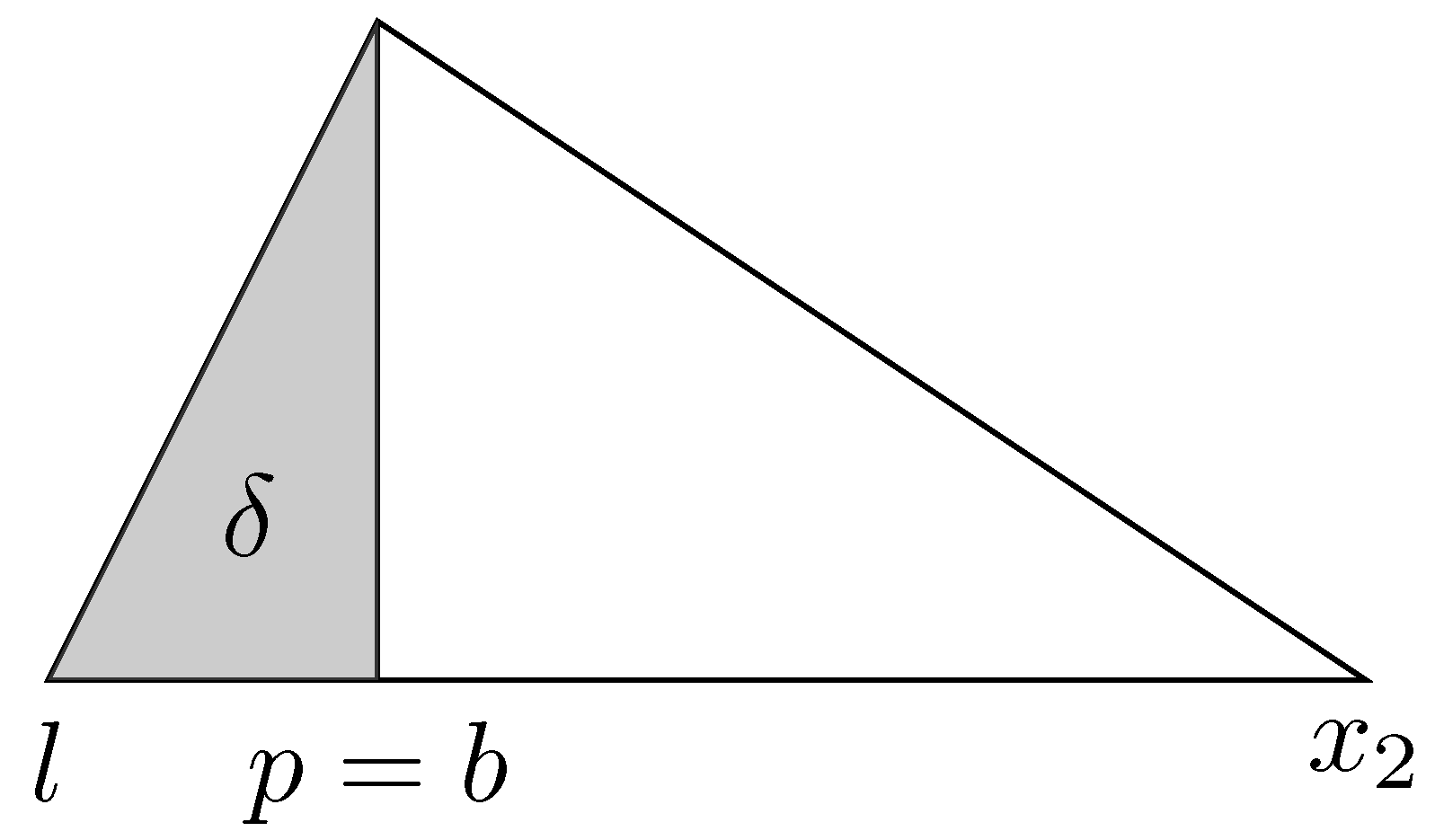
I fit triangular distributions for those respondents filling two adjacent intervals.10 Again, I allow the distribution to be a scalene triangle with the mode of the distribution coinciding with the respondent’s point estimate.11 When fitting triangular distributions over two intervals, one of the endpoints of the distributions is fitted to either the rightmost point of the higher interval or the leftmost point of the lower interval. The other endpoint is determined from the restricted endpoint, the assumed mode of the distribution, and the probabilities placed in each bin. Denote the mode of the distribution as p and upper and lower bounds of the distribution as l and r, respectively. The height of the distribution is given by . The subjective distribution for an individual is therefore given by:
Two adjacent bins will have respective endpoints and . Denote the consumer’s point estimate as p. Denote the probability in the lower bin as . The restricted and fitted endpoints will be determined by a combination of the relative widths of the two bins, , and the position of p relative to b. To keep the probability under the subjective distribution in the bins to which the respondent assigned it, the mode is sometimes adjusted. In some cases, I attempt to fit the left endpoint and solve for the right endpoint only in the event that solutions for the left endpoint fall outside of the lower interval. In other cases, I attempt to fit the right endpoint first. Should the right endpoint fall outside the upper interval, I fit the left endpoint next.
Appendix A.2.1. Pin Right Endpoint r = x2, Solve for l
Cases in which I solve for the left endpoint first include:
- Lower bin has smaller probability, , bins are of equal width
- Lower bin has smaller probability, , lower bin is narrower, both bins are bounded
- Lower bin has smaller probability, , lower bin is wider, both bins are bounded
- Higher bin has smaller probability, , lower bin is wider, both bins are bounded
- Even weight in two bins (), lower bin is wider, both bins are bounded
- Even weight in two bins (), bins are of equal width, point estimate falls in lower bin
- Weight falls in the lowest bin, which is unbounded
- p = b
Call the probability in the leftmost bin . If the point estimate, p, falls at the breakpoint between the two bins,
Figure A1.
Point estimate at bin breakpoint.

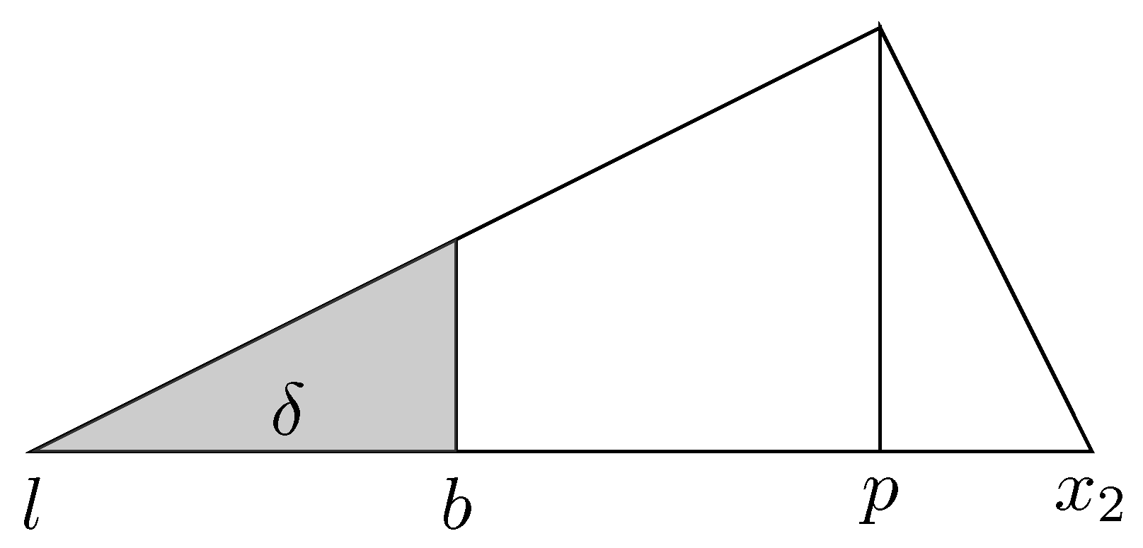
- p > b
When p falls above the point separating the two bins, l is the solution to the following quadratic that falls within :
Figure A2.
Point estimate in higher bin.

Such a case is shown in Figure A2.
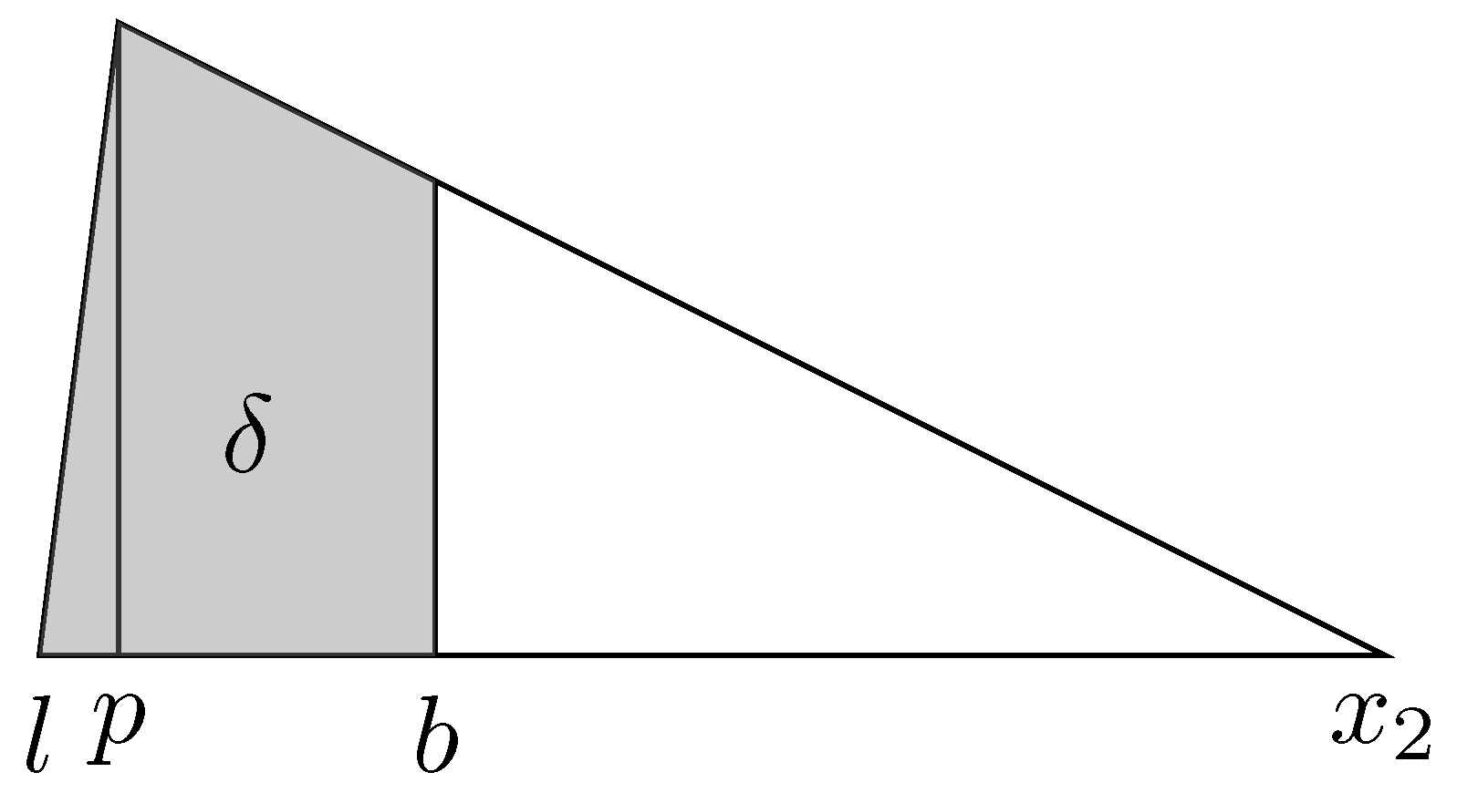
- p < b
If the point estimate falls in the lower bin, the left endpoint of the triangle is:
Figure A3.
Point estimate in lower bin, Case 1.

The exception to this is the case where the solution to l is greater than the point estimate (putting the point estimate outside of the fitted distribution). In this case, the left endpoint is given by:
Figure A4.
Point estimate in lower bin, Case 2.

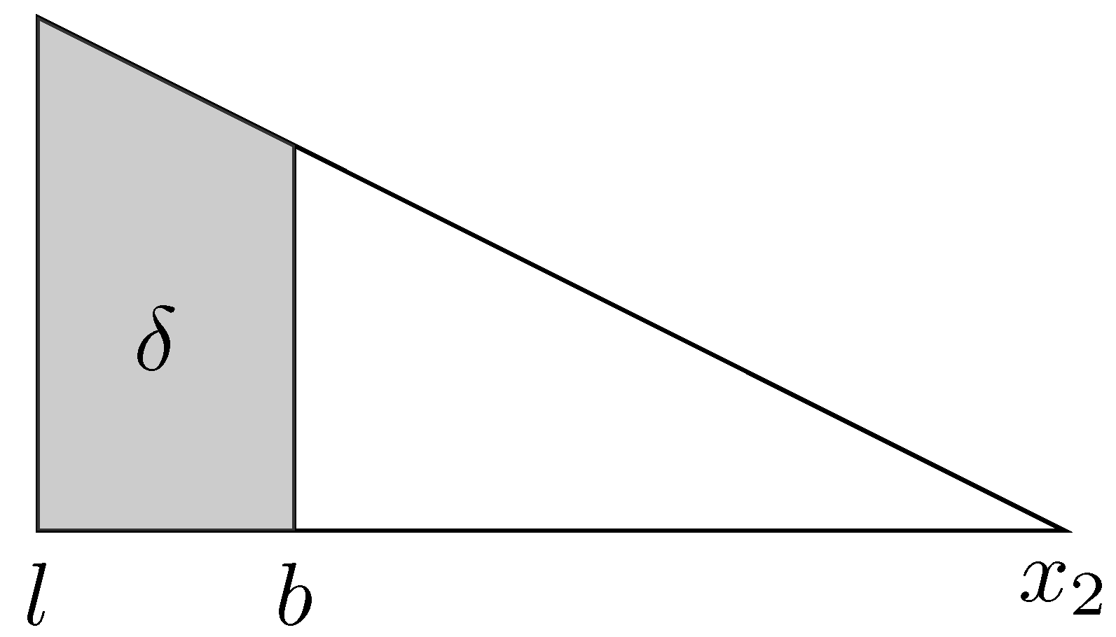
Appendix A.2.2. Pin Left Endpoint, l = x1, Solve for r
Cases in which I solve for the right endpoint first include:
- Higher bin has smaller probability, , bins are of equal width;
- Higher bin has smaller probability, , higher bin is narrower, both bins are bounded;
- Higher bin has smaller probability, , higher bin is wider, both bins are bounded;
- Lower bin has smaller probability, , higher bin is wider, both bins are bounded;
- Even weight in two bins (), higher bin is wider, both bins are bounded;
- Even weight in two bins (), bins are of equal width, point estimate falls in higher bin ;
- Weight falls in highest bin, which is unbounded.
- Call the probability in the rightmost bin . If the point estimate, p, falls at the breakpoint between the two bins, the right endpoint is given by:
- If the point estimate falls in the lower bin, r is the solution to the following quadratic that falls within :
Appendix A.3. Case 3—Consumer Uses Three or More Intervals
When the consumer places positive probability to three or more intervals, I fit a generalized beta distribution with endpoints l and r and shape parameters and following Engelberg. As in overview, I fix l and r to the minimum and maximum bounds of the intervals with positive probability.12 The probability distribution is given by:
where . I assume that the individual’s point estimate is equal to the mode of their distribution, which given by . If the respondent’s point estimate falls outside of the range l to r, I set p equal to the value of l or r closest to the reported point estimate. The imposition of the point estimate as the mode of the distribution creates a further relationship between and . Given these requirements, I fit the shape parameters (and bounds in the case of unbounded intervals) as in the overview, fitting a minimum distance estimator that minimizes the distance between the observed probability distribution and the probability distribution generated by the proposed parameter combinations.
| 1 | “I am attentive to the risk that inflation pressures could broaden or prove persistent, perhaps as a result of wage pressures, persistent increases in rent, or businesses passing on a larger fraction of cost increases rather than reducing markups, as in recent recoveries. There are risks on both sides of the outlook. There are upside risks to consumption spending associated with the high level of households’ savings. There are downside risks associated with the Delta variant.” Lael Brainard, July 2021. |
| 2 | The historical values of diffusion indexes for the change in real GDP, the unemployment rate, and PCE and core PCE inflation appeared first in the December 2020 SEP. The value of diffusion index is given by the share of participants who respond that risk weighting around their projection is “Weighted to the Upside” minus the share that respond “Weighted to the Downside”. |
| 3 | “Monetary policy responded first in the summer of 2012 by acting to defuse the sovereign debt crisis, which had evolved from a tail risk for inflation into a material threat to price stability.” Speech by Mario Draghi, President of the European Central Bank, at the ECB Forum on Central Banking, Sintra, 18 June 2019. |
| 4 | The SCE publishes a measure of expected inflation derived from probabilistic forecasts. Their current method for fitting subjective probability forecasts produces symmetric distributions by construction for roughly 30% of responses, attenuating the measurement of asymmetry in subjective distributions over future inflation. Given the Federal Reserve’s recent emphasis on the asymmetry of its public forecasts, measures of private expectations should allow for such asymmetry, as the measure I propose does. |
| 5 | This selection of inflation or deflation is based on the answer to a previous question. |
| 6 | There are 35,676 and 33,705 unique histogram forecasts and 52,922 and 51,809 unique forecasts for short run and medium run ahead inflation, respectively. |
| 7 | In the case that a forecaster places the same maximum probability in multiple bins, a modal point forecast can fall in the range of any of these bins. |
| 8 | The SCE currently publishes medians rather than means to avoid the influence of outliers and I follow this. |
| 9 | When a survey respondent places all probability in an unbounded interval, the SCE assumes bounds of and 38. I follow this convention. |
| 10 | Include number not doing this. |
| 11 | The mode is, in certain cases, modified to allow the probabilities in each interval under the fitted distribution to match the probabilities that the consumer assigned to those intervals. In any situation where the mode differs from the reported point estimate, I choose the value of the mode that is both consistent with the reported probabilities and closest to the reported point estimate. |
| 12 | If the positive probability intervals include the unbounded intervals, I allow the relevant bound(s) to be estimated along with the shape parameters. Following the overview, I allow a maximum value of 38 for r and a minimum value of −38 for l. |
References
- Adams, Patrick A., Tobias Adrian, Nina Boyarchenko, and Domenico Giannone. 2021. Forecasting Macroeconomic Risks. International Journal of Forecasting 37: 1173–91. [Google Scholar] [CrossRef]
- Alessandri, Piergiorgio, and Haroon Mumtaz. 2019. Financial regimes and uncertainty shocks. Journal of Monetary Economics 101: 31–46. [Google Scholar] [CrossRef] [Green Version]
- Andrade, Philippe, Eric Ghysels, and Julien Idier. 2012. Tails of Inflation Forecasts and Tales of Monetary Policy. Paris: Banque de France. [Google Scholar]
- Andrade, Philippe, Valère Fourel, Eric Ghysels, and Julien Idier. 2014. The Financial Content of Inflation Risks in the Euro Area. International Journal of Forecasting 30: 648–59. [Google Scholar] [CrossRef] [Green Version]
- Apergis, Emmanuel, and Nicholas Apergis. 2021. Inflation expectations, volatility and COVID-19: Evidence from the US inflation swap rates. Applied Economics Letters 28: 1327–31. [Google Scholar] [CrossRef]
- Armantier, Olivier, Giorgio Topa, Wilbert van der Klaauw, and Basit Zafar. 2016. An Overview of the Survey of Consumer Expectations. Federal Reserve Bank of New York Staff Reports 800: 51–72. [Google Scholar]
- Bernanke, Ben. 2006. Board of Governors. Washington, DC: Remarks. [Google Scholar]
- Binder, Carola. 2020. Coronavirus Fears and Macroeconomic Expectations. The Review of Economics and Statistics 102: 721–30. [Google Scholar] [CrossRef]
- Boon, Martijn, Fernando Duarte, Frans de Roon, and Marta Szymanowska. 2020. Time-varying inflation risk and stock returns. Journal of Financial Economics 136: 444–70. [Google Scholar] [CrossRef] [Green Version]
- Bowley, Arthur Lyon. 1920. Elements of Statistics. New York: Charles Scribner’s Sons. [Google Scholar]
- Chaudhary, Manav, and Benjamin Marrow. 2022. Inflation Expectations and Stock Returns. SSRN. [Google Scholar] [CrossRef]
- Coibion, Olivier, Yuriy Gorodnichenko, Saten Kumar, and Jane Ryngaert. 2021. Do You Know that I Know that You Know? Higher-Order Beliefs in Survey Data. Quarterly Journal of Economics 136: 1387–446. [Google Scholar] [CrossRef]
- D’Acunto, Francesco, Ulrike Malmendier, and Michael Weber. 2022. What Do the Data Tell Us About Inflation Expectations? In The Handbook of Economic Expectations. Edited by Ruediger Bachmann, Giorgio Topa and Wilbert van der Klaauw. Cambridge: Academic Press, pp. 133–62. [Google Scholar]
- D’Amico, Stefania, and Athanasios Orphanides. 2008. Uncertainty and Disagreement in Economic Forecasting. Divisions of Research and Statistics and Monetary Affairs, Federal Reserve Board 56: 1–39. [Google Scholar] [CrossRef]
- Engelberg, Joseph, Charles F. Manski, and Jared Williams. 2009. Comparing the Point Predictions and Subjective Probability Distributions of Professional Forecasters. Journal of Business and Economic Statistics 27: 30–41. [Google Scholar] [CrossRef]
- Fleckenstein, Matthias, Francis A. Longstaff, and Hanno Lustig. 2017. Deflation Risk. The Review of Financial Studies 30: 2719–60. [Google Scholar] [CrossRef]
- Galati, Gabriele, Richhild Moessner, and Maarten van Rooij. 2021. The Anchoring of Long-Term Inflation Expectations of Consumers: Insights from a New Survey. BIS Working Papers 936: 1–44. [Google Scholar]
- Garcia, Juan A., and Andrés Manzanares. 2007. Losing the Inflation Anchor. What Can Probability Forecasts Tell Us about Inflation Risks? ECB Working Paper 734. [Google Scholar] [CrossRef]
- Gimeno, Ricardo, and Alfredo Ibáñez. 2018. The eurozone (expected) inflation: An option’s eyes view. Journal of International Money and Finance 86: 70–92. [Google Scholar] [CrossRef] [Green Version]
- Kilian, Lutz, and Simone Manganelli. 2008. The Central Bank as a Risk Manager: Quantifying and Forecasting Inflation Risks. Journal of Money, Credit and Banking 40: 1103–29. [Google Scholar] [CrossRef]
- Kumar, Saten, Hassan Afrouzi, Olivier Coibion, and Yuriy Gorodnichenko. 2015. Inflation Targeting Does Not Anchor Inflation Expectations: Evidence From Firms in New Zealand. Brookings Papers on Economic Activity 2015: 151–225. [Google Scholar] [CrossRef] [Green Version]
- Lopez-Salido, David, and Francesca Loria. 2022. Inflation at Risk. Washington, DC: Board of Governors of the Federal Reserve System. [Google Scholar] [CrossRef]
- Natoli, Filippo, and Laura Sigalotti. 2018. Tail Co-movement in Inflation Expectations as an Indicator of Anchoring. International Journal of Central Banking 14: 35–17. [Google Scholar] [CrossRef]
- Orphanides, Athanasios, and John Williams. 2007. Imperfect Knowledge, Inflation Expectations, and Monetary Policy. In The Inflation Targeting Debate. Edited by Ben Bernanke and Michael Woodford. Chicago: The University of Chicago Press, pp. 201–48. [Google Scholar]
- Reis, Ricardo. 2021. Losing the Inflation Anchor. Brookings Papers on Economic Activity, 307–61. Available online: https://ssrn.com/abstract=3960248 (accessed on 15 January 2022).
- Rich, Robert, and Joseph Tracy. 2021. A Closer Look at the Behavior of Uncertainty and Disagreement: Micro Evidence from the Euro Area. Journal of Money, Credit, and Banking 53: 233–53. [Google Scholar] [CrossRef]
- Rich, Robert W., Joseph Song, and Joseph S. Tracy. 2012. The Measurement and Behavior of Uncertainty: Evidence from the ECB Survey of Professional Forecasters. Federal Reserve Bank of New York Staff Reports 588. [Google Scholar] [CrossRef] [Green Version]
- Ruge-Murcia, Francisco J. 2003. Inflation Targeting under Asymmetric Preferences. Journal of Money, Credit and Banking 35: 765–85. [Google Scholar] [CrossRef]
- Vukovic, Darko B., Moinak Maiti, and Michael Frömmel. 2022. Inflation and Portfolio Selection. Finance Research Letters 50: 103202. [Google Scholar] [CrossRef]
Figure 1.
The figure shows the survey-interpolated medians of the distribution implied means for each short run and medium run inflation expectations. The means are calculated using the subjective probability distribution proposed in this paper.
Figure 1.
The figure shows the survey-interpolated medians of the distribution implied means for each short run and medium run inflation expectations. The means are calculated using the subjective probability distribution proposed in this paper.

Figure 2.
The figure shows measures of cross-sectional disagreement and subjective uncertainty for short run and medium run inflation expectations. The dispersion is calculated as the difference in the interquartile range across the individual implied means in a period. The subjective uncertainty measure is the interpolated median of the interquartile ranges of the individual subjective distributions.

Figure 3.
This figure shows the fitting methods for respondents placing positive probability in one or two bins. The first column compares unique forecasts that share an identical one-bin histogram but that have different point estimates. The second column shows forecasts that all have the same point estimates but place differing probabilities across the same two bins. The Survey of Consumer Expectations distribution is shown in solid gray while the distribution fitted using the approach described in this paper is shown in partly transparent blue. The modified approach allows for asymmetric probability distributions in those who report probability in only two bins, in contrast to the approach of (Engelberg et al. 2009 and Armantier et al. 2016) who impose symmetry on these distributions. More than 30% of forecasters fill one or two bins for both one-year and three-year forecasts, meaning that the relaxation of the assumption of symmetry will impact a large number of observations.

Figure 4.
The figure shows the diffusion indexes of the assessed risk weighting around short run and medium run projections. It is calculated by, for each month, subtracting the survey-weighted share of participants whose distributions are negatively skewed from the share of participants with positively skewed distributions.


Table 1.
The table provides the survey-weighted means of measures of short run and long-run inflation expectations—the implied means and medians of the subjective distributions derived as in Section 3. In addition, the survey-weighted means of the IQR, skewness and left and right tails implied by the subjective probability distributions over short run inflation are included.
| Survey-Weighted Mean | |
|---|---|
| Short Run Expectations | |
| 4.22 | |
| (0.02) | |
| 4.25 | |
| (0.02) | |
| 5.49 | |
| (0.02) | |
| 0.00 | |
| (0.00) | |
| 2.82 | |
| (0.01) | |
| 2.97 *** | |
| (0.01) | |
| Medium Run Expectations | |
| 4.08 | |
| (0.02) | |
| 4.04 | |
| (0.02) |
Standard errors in parentheses. *** p < 0.01.
Table 2.
The table shows the results from regression Equations (4) and (5). The results show that longer run expectations increase with the skewness of short run distributions—as perceived risks become weighted to the upside—and with the tails—as perceived inflationary and disinflationary risks become more extreme—of the short run distribution.
| 0.62 *** | 0.62 *** | |
| (0.00) | (0.00) | |
| −0.02 *** | −0.04 *** | |
| (0.00) | (0.01) | |
| 1.47 *** | 0.25 | |
| (0.12) | (0.16) | |
| 0.13 *** | ||
| (0.01) | ||
| −0.07 *** | ||
| (0.01) | ||
| Observations | 105,095 | |
| Fixed Effects | Yes | Yes |
| Hausman p-Value | 0.00 | 0.00 |
Standard errors in parentheses. *** p < 0.01.
Table 3.
The table shows the results from regression Equation (7). The results show that, on average, consumers’ concerns about upside tail risk increase when short run expectations increase.
Table 3.
The table shows the results from regression Equation (7). The results show that, on average, consumers’ concerns about upside tail risk increase when short run expectations increase.
| 0.06 *** | |
| (0.01) | |
| −0.04 *** | |
| (0.01) | |
| 0.48 *** | |
| (0.08) | |
| Constant | −0.10 *** |
| (0.03) | |
| Observations | 103 |
| F | 30.88 |
| 0.48 | |
| Breusch-Pagan p-value | 0.8578 |
Standard errors in parentheses. *** p < 0.01.
Disclaimer/Publisher’s Note: The statements, opinions and data contained in all publications are solely those of the individual author(s) and contributor(s) and not of MDPI and/or the editor(s). MDPI and/or the editor(s) disclaim responsibility for any injury to people or property resulting from any ideas, methods, instructions or products referred to in the content. |
© 2023 by the author. Licensee MDPI, Basel, Switzerland. This article is an open access article distributed under the terms and conditions of the Creative Commons Attribution (CC BY) license (https://creativecommons.org/licenses/by/4.0/).
Share and Cite
MDPI and ACS Style
Ryngaert, J.M. Balance of Risks and the Anchoring of Consumer Expectations. J. Risk Financial Manag. 2023, 16, 79. https://doi.org/10.3390/jrfm16020079
AMA Style
Ryngaert JM. Balance of Risks and the Anchoring of Consumer Expectations. Journal of Risk and Financial Management. 2023; 16(2):79. https://doi.org/10.3390/jrfm16020079
Chicago/Turabian StyleRyngaert, Jane M. 2023. "Balance of Risks and the Anchoring of Consumer Expectations" Journal of Risk and Financial Management 16, no. 2: 79. https://doi.org/10.3390/jrfm16020079