Understanding the Effects of Market Volatility on Profitability Perceptions of Housing Market Developers

Abstract

Drastic shifts in prices and housing market trends in recent years, representing shocks to the housing system, have led many residential developers to pause or cancel their projects. In the already heated housing markets of the Greater Toronto Area (GTA), these supply frictions can have ramifications for affordability. Our study formulates a standardized “proforma” model of the profitability of a hypothetical condominium project in the city of Toronto, Canada, scheduled between 2019 to 2023, to explore the combined effect of developers’ price expectations and market volatility on developers’ decisions. Using the proposed proforma, we first identify the key drivers of development decisions. We then evaluate the impact of the expectation formation of key factors influencing perceived development profitability, including construction costs, sales prices, and interest rates, on the financial feasibility of potential developments. The results highlight that boundedly rational expectations can cause variations in profitability perceptions and potentially reverse development decisions in volatile market conditions. Our results highlight the sources of risk and uncertainty in development decisions, facilitating the recognition of possible solutions to mitigate these risks and increase affordable housing supplies. The proposed model can also enhance the realism of decision models in agent-based representations of land and housing markets.

1. Introduction

As housing markets continually evolve, influenced by factors such as economic volatility, demographic shifts, and policy changes, traditional models of land and housing prices often prove inadequate in their ability to fully grasp the multifaceted complexities and nuances of these developments, failing to accurately predict housing prices and development trends (Hunt et al. 2005; Wegener 2021). Further, as argued by Lee and Reed (2014) in a comprehensive review of the literature on housing market volatility, housing policy analysis should consider impacts on housing price volatility and associated market uncertainty. Volatile housing prices can disrupt market equilibrium, affecting affordability, home ownership, investment decisions, and overall housing supply. Understanding and quantifying this volatility provides policymakers with crucial insights into the dynamics of housing markets, enabling them to design interventions that can mitigate the adverse effects of market swings, such as policies that provide subsidies for first-time buyers (Lee and Reed 2014). However, the models historically used to measure housing price volatility at a macro-economic scale show predictive limits. A comparison between the forecast performance of widely used univariate time series methods when applied to housing prices suggested that while GARCH models exhibit strong predictive performance in forecasting stationary volatility, their efficacy may diminish when confronted with significant regime changes (Crawford and Fratantoni 2003).

One of the primary challenges models of housing market volatility face is a reliance on aggregate historical data and simplistic assumptions that inadequately account for the dynamic nature of the housing market (Bishop et al. 2020; Ho et al. 2021; Liu et al. 2020; Pai and Wang 2020). Economic events, such as recessions or unexpected shocks to the market, can swiftly alter the landscape, rendering past data less relevant (Balemi et al. 2021). Moreover, expectations in the market arise from, and consequently influence, the historical trajectory of land transactions and realized prices (Filatova 2015; Leung et al. 2009; Taltavull and McGreal 2009), impacting the actors’ financial perceptions, especially in volatile market conditions (Kuchler et al. 2023).

Spatial and temporal variability, combined with rapid demographic changes, present other significant challenges to modelling housing prices and market supply (Jeanty et al. 2010; Yang et al. 2020b). The ever-evolving nature of housing market and policy regulations, with price trends and supply dynamics differing markedly from one location to another, are subject to rapid changes over time and can further complicate predictions, as they can have substantial impacts on supply-and-demand dynamics (Salvati et al. 2019; Yang et al. 2020a). Furthermore, demographic changes, including shifts in population growth, urbanization trends, and generational preferences, introduce new dimensions of uncertainty that can drastically impact housing prices and cause market volatility by influencing the housing preferences and demand for different housing products (Engelhardt and Poterba 1991; Gong and Yao 2022). Factors driving prices and supply can transform abruptly, necessitating models that are both flexible and adaptive.

Microsimulation models offer promise to address these heterogeneous dynamics, but their success in modelling housing supply and prices is mixed. For instance, the ILUMASS model, aimed at creating a fully microscopic model of urban land use, transport, and environment for the metropolitan area of Dortmund, could not prove an adequate level of accuracy in predicting housing prices and market supply (Wagner and Wegener 2007), due in part to simplistic assumptions on individual decision-making that could not capture spatial and temporal variability. Through experimenting with a generalized Agent-Based Model of land use and housing applied in the USA, Laos, and China, Magliocca et al. (2014a) showed missing mechanisms and simplistic assumptions in the representation of real-world land-use dynamics, such as the underlying labour- and risk-minimizing decision-making frameworks, that can lead to failures in simulating land-use patterns and prices, causing the models to fall short in forecast performance.

This study is motivated by a growing need for more advanced and adaptable models that can better account for the real-world intricacies and uncertainties inherent in land-use and housing price forecasting to improve the current projections of prices and housing supply. While price expectations are an essential factor in shaping the asking prices and transaction values of properties in land and housing markets (Filatova 2015; Taltavull and McGreal 2009), the majority of the current models of land and housing markets do not consider the effect of actors’ expectations in their behaviours and decisions (Martin et al. 2021; Taltavull and McGreal 2009), diminishing their ability to predict market trends and capture the effect of market shifts, especially in volatile market conditions. For instance, the integrated land use–transport microsimulation model for the Paris Region (SIMAURIF) showed significant challenges in modelling land and housing markets. While the model could forecast housing prices at an aggregate level, it failed to predict housing supply and market prices at the cell level due to a lack of detail in modelling socioeconomic components and actors’ behaviours (Nguyen-Luong 2008).

Our study explores the impact of alternative theoretical financial perceptions of housing market developers on the financial analyses that support real-world housing supply decisions. The inclusion of such models can be transformative for models of land and housing markets by providing a more realistic representation of developers’ financial perceptions and how changes in these perceptions in response to price shocks can abruptly shift housing supply. In essence, more enhanced models of land and housing markets can shed light on the relationships between housing supply and volatile cost and revenue price dynamics, empowering policymakers and planners to navigate the complexities of the contemporary housing landscape and develop strategies that foster sustainable and equitable housing markets.

Since the late 1990s, there has been an extraordinary proliferation of condominium developments across the Greater Toronto Area (GTA), Canada, as shown in Figure 1, fueled by an influx of private investments in condominium stock and government-sponsored redevelopment of social housing (Lehrer et al. 2010). Private developers have significantly increased the vertical residential space in the housing landscape by pursuing significant re-zonings related to building height and land uses (Buckley and Brauen 2022). In recent years, however, in spite of housing supply shortages in Canada’s largest metropolitan areas, including the GTA, Toronto has experienced a cascade of cancellations of new condominium projects as a result of major shifts in housing market dynamics (Feinstein 2023; Fox 2022; Sherman 2022; Younglai 2022) (see Figure 2).

Alterations in development projects and supply decisions can be traced back to the behaviour of housing market developers, who base development decisions on their expectations of market trends, such as construction costs and potential demand for different housing products. Developers and other key market actors such as lenders seek to maximize their profit from potential developments according to their perception of market conditions, such as rising interest rates (Bank of Canada 2023). This behaviour of residential developers to undertake potential developments aligns with the notion of economic rationality (Magliocca et al. 2014b; Mohamed 2006). However, if developers are fully rational, why do sudden cost and revenue changes take them by surprise and lead to major changes in project plans?

While more than 260,000 housing projects were started in Canada in 2022, this supply rate is insufficient. Although Canada is projected to build 2.3 million new homes by 2030, CMHC (2022, 2023b) estimates that it actually needs to build an additional 3.5 million homes to restore housing affordability by 2030, with around 1.5 million additional homes needed in Ontario alone. Currently, around half the construction activity in major centres where demand is greatest, such as Toronto and Vancouver, is in the condominium and rental segments. This number will only continue to grow over time given that apartment living is generally less expensive per unit than ground-facing options, even considering the relatively high-rise construction costs. Municipalities also continue to seek high-density housing to minimize urban expansion and create critical mass for transit projects. Financing models for high-rise development are also well-developed. Thus, high-rise condominiums and rental construction in high-demand areas can be a pragmatic approach to providing more housing options. As this trend gains momentum, understanding the factors that impact high-rise developer supply decisions is critical to help inform governments at all levels on what policies may be needed to incentivize the construction of more high-density housing.

Developers’ expectations with regard to factors such as construction costs, interest rates, and market prices are critical drivers of the decision to supply housing. Developers use a financial analysis tool, called “proforma,” to estimate the financial return from the potential developments and reach development decisions (Barer 2011; Hollander and Stephens 2023; Jennings 2012; Murray 2022). Developers and their investors require these proformas to assess the profitability of a new development when deciding if, when, and where they should begin new high-rise projects. Volatile macroeconomic conditions can represent a shock to the housing system, leading to uncertainty and volatility in the new housing supply. This uncertainty heightens the investment risk for developers and investors, which can increase the required return on investment to offset the perceived risks.

To mitigate the uncertainties in financial projections, developers often rely on cost consultants, who possess a wealth of historical data derived from comparable projects (Betts 1991; Okwilagwe and Apostolakis 2017; Smyth 2005). These seasoned actors play a pivotal role in establishing parameters for prospective developments, offering a perceived higher degree of reliability in the estimation of forthcoming prices and costs (Wood and Ellis 2003). Nevertheless, we argue that it is impossible for even seasoned actors to perfectly predict market trends, especially in volatile market conditions.

Additionally, given that the development of high-rise residential buildings are long-term endeavours, builders need to price their projects at the early phase of their sales and marketing campaigns. However, projects will not usually break ground until 24 months after a condo sale is registered, leading to significant risk if expectations around costs prove incorrect. This can lead to project delays and cancellations as projects become less economically viable. The recent run-up in labour and building material costs coming out of the pandemic is a case in point. According to Urbanation data, shown in Figure 2b, approximately 10,000 condominium units in Toronto have been cancelled in recent years.

This paper aims to address the following research questions:

• What are the main factors impacting the profitability perceptions of potential high-rise developments?
• How do profitability perceptions shift when boundedly rational price expectations are used to project market trends for construction costs, unit sales prices, and interest rates?
• Can boundedly rational expectations of market trends explain project cancellations, when the housing system experiences unanticipated price shocks?

To address these research questions, our paper explores the key drivers of the profitability of development projects, using a hypothetical prototype proforma to identify the relative influence of cost and revenue factors on development returns and which factors most influence a development’s profitability. We assume that such factors will be primary drivers of the development decisions of housing market developers. To this end, we formulated a standardized proforma representing the essential financial elements of sales development projects, including project financing, potential revenues, and costs. We examined the sensitivity of the Net Present Value (NPV) and Internal Rate of Return (IRR) of the project to various model parameters to evaluate the role of different proforma assumptions on the financial profitability of the project. This analysis highlights the importance of three factors that have shown unexpected volatility in recent years, construction costs, unit sales prices, and interest rates.

We then evaluated the impact of the boundedly rational expectation formations of developers on their development decisions. Developers, like all human actors, lack perfect foresight of future economic conditions. To account for this limited foresight, we identified several expectation formation models based on the review of the literature and incorporated these models into the proposed proforma. Inclusion of these mechanisms allows us to further explore how different decision strategies and expectation formations of primary factors influencing the financial analysis of a potential development project, including construction costs, unit sales prices, and interest rates, influence profitability thresholds for new developments.

The rest of this paper is organized as follows: Section 2 discusses the literature on developer decisions and their price expectations, also highlighting the key factors influencing the financial profitability of projects and the development decisions of housing market developers. Section 3.1 presents the formulation of a standardized sales proforma as a financial analysis tool that uses the Net Present Value (NPV) and the Internal Rate of Return (IRR) as the primary measures to evaluate the profitability of potential development projects. Section 3.2 discusses the application of the proposed proforma to a case study of a hypothetical potential condo project in the city of Toronto, scheduled between July 2019 and June 2023, to showcase the impact of various factors on development decisions. Section 4.1 presents the results of numerical sensitivity analyses with several model parameters to identify key drivers of the project’s profitability calculations. Section 4.2 explores how boundedly rational price expectations and correlation between decision parameters can explain project postponement and cancellation based on profitability perceptions in volatile market conditions. Finally, Section 5 discusses the policy implications and introduces future model applications.

2. Literature Review

Perspectives on developers’ economic rationality. Various perspectives have been used to describe the behaviours and expectation formation of developers in land and housing markets. The “rational expectations” economic model assumes that developers will best use all available information to precisely estimate future price trends. However, the “complexity economics” (Arthur 2018) point of view argues that economic actors can behave at best as boundedly rational, as the real world is too complex to predict all outcomes. Some studies qualitatively characterize developers as profit-seeking, risk-taking, and innovative (Maruani and Amit-Cohen 2011; Winarso 2000), while other studies find evidence of “boundedly rational” decision behaviour, including satisficing (the tendency to find and select the closest satisfactory solution), loss aversion (weighing losses more than gains), and weighing relative rather than absolute wealth shifts (prospect theory) (Magliocca et al. 2014b).

Primary factors in development decisions of developers. Developers rely on their expectations of future market trends and profitability perceptions to decide on their actions. For instance, high risk perceptions of project failure combined with low expectations of resident demand can lead to under-supply of particular housing typologies, such as “Missing Middle” housing, referring to low-rise high-density homes such as duplexes, triplexes, and townhouses (Parker et al. 2023). On the other hand, expectations of land up-zoning coupled with expectations of high demand by investors can trigger oversupply of products such as small high-rise condos. Both trends have recently been observed in Ontario land and housing markets (Parker et al. 2023; Paull 2022; Sarnoff 2022).

Proformas allow developers to test the revenue and cost assumptions for potential development projects to evaluate whether they support a decision to purchase land and/or develop housing. Proformas help private developers evaluate the financial viability of the development projects and achieve the “highest and best use” for a potential project (Johnson et al. 2018). Development proformas consider financing options (e.g., equity and debt funds), market analytics (e.g., sales prices and construction costs), and planning requirements (e.g., density requirement and development typologies), to assess the revenue generation and opportunity costs (the potential return on alternative investments). The use of development proforma to represent developers’ decision-making is consistent with a hypothesis that developers are boundedly rational profit maximizers (Magliocca et al. 2014b, 2011).

To arrange the financial aspects of projects using proforma, housing market developers face a range of significant market and planning risks, influencing their development decisions regarding new housing projects. Developer–investor relationships fraught with planning dynamics and tensions interact to create or inhibit financing opportunities for the new developments (Brill 2022). Financing costs and the financial feasibility of development projects can also be significantly impacted by the fluctuations in interest rates, since they directly influence the cost of borrowing money for development projects. Developers need to carefully consider interest rate trends and potential risks when structuring their financing strategies to effectively manage financial risks.

Previous observations of market trends have shown that interest rates can impact the housing market in several ways, as shown in Figure 3. An increase in interest rates can influence housing demand by reducing affordability, which in turn can have a suppressing effect on unit sales prices (Chong 2023; Justiniano et al. 2019; Sutton et al. 2017). In such a situation, the profitability of the project is significantly impacted by the shifts in the two variables. On the cost side, the increasing interest rates would increase the project financing costs, imposing extra financial burden on the project. On the revenue side, depressing housing prices would decrease the expected revenue for the projects, implying that the project might not achieve its expected financial goal Arslan (2014); Chong (2023). Therefore, understanding the association between interest rates and housing prices is crucial for housing market developers when considering market volatility and financial return from potential developments.

In addition to interest rates, various market factors, such as construction costs, sales price appreciation and volatility, and pricing of land options, guide developers’ expectations of financial viability and subsequent land development decisions (Cunningham 2007; Felsenstein and Ashbel 2010; Filatova et al. 2009; Imrie and Street 2009; Silva 2002; Taltavull and McGreal 2009). Construction costs can impose a significant financial barrier to development projects. In the early stage of the project, developers must rely on their initial construction cost expectations for their development decisions. However, those expectations may be based on limited information and have a high degree of uncertainty (Jennings 2012; Koo et al. 2011). As the project proceeds, the construction costs are updated based on the available information about the development, and incoming information may alter the viability of the project.

Other market trends, such as sale and rent price trends, the vacancy and absorption rates (i.e., how quickly new builds are rented or sold when completed), and land pricing options, can also influence developers’ estimation of the generated revenue in their potential development projects (Antczak-Stępniak 2021; Huang 2020; Murray 2022). For instance, a local increase in housing and land supply can lead to a decline in absorption rates, which impacts the expected revenues from the project and could be a signal for developers to alter their decisions about land developments (Barer 2011).

Modelling the price expectation of housing market developers. Our review of the literature indicates that the majority of studies on price expectations have employed statistical Huang et al. (2021); Taltavull and McGreal (2009) or agent-based models (Ettema 2011; Gilbert et al. 2009; Magliocca et al. 2011; Parker and Filatova 2008) of land and housing markets, as modelling boundedly rational price expectations and their interactions is challenging or impossible using analytical approaches. Leung et al. (2009) assumed that housing market developers could develop heterogeneous boundedly rational expectations, including naive expectations, biased beliefs, trend-following expectations, and adaptive expectations. Another perspective characterizes the adaptation of price expectation models from the financial agent-based literature (Arthur 1994, 2006; Axtell 2005). Magliocca et al. (2011) evaluated the conversion of farmland to housing developments over time by developing an ABM housing and land market model in which developers use adaptive price expectations to predict the next period’s price based on current and past price information. Agents use a set of different prediction methods, such as the mean model, the cycle model, and the projection model, and select the prediction model with the least error to make pricing decisions in the current period.

Another group of studies, mainly from the literature on finance and general economics, have conducted experiments with human subjects (e.g., learning-to-forecast experiments) to understand price expectations in a controlled setting (Hommes 2021). For instance, Hommes et al. (2005) conducted four rounds of experiments in a laboratory setting to evaluate the individual expectations of asset prices. The findings highlighted that as the experiment progresses, the subjects use more complicated strategies to form expectations, helping them improve their learning and convergence over the rounds. Bao and Hommes (2015) designed an experimental housing market and evaluated the effect of the price elasticity of supply on market stability. They used learning-to-forecast experimental analysis to study individual decisions and housing price expectations and their impact on market stability. The experiments indicated that speculators rely on trend-following expectations in the absence of endogenous housing supply, where the housing demand does not add negative feedback to the market prices, leading to significant market bubbles and crashes. Although this group of studies explored the expectation formation of human subjects regarding asset prices, the results of the experiments and proposed models cannot comprehensively reflect the behaviour of housing market developers as the experiments are not originally designed to evaluate the developers’ behaviours in the land and housing markets.

Conclusions from literature review. Review of the literature indicated that there is a gap in the study of decision strategies of housing market developers through understanding their profitability perceptions and price expectations. Moreover, to our knowledge, diverse approaches to representing developer expectations have not been explored and compared within the same model. To fill this gap, our study identifies the important drivers of development decisions by formulating and exploring a standardized proforma as a financial model used to assess the financial viability of potential development projects. To account for the impact of the price expectations of developers on their development decisions, we incorporated various models of expectation formation into the proposed proforma to explain the boundedly rational behaviour of housing market developers regarding the projection of market trends that primarily influence a 320.90project’s profitability, including construction costs, unit sales prices, and loan interest rates. Our study establishes an understanding of the development proforma and primary factors contributing to the financial viability of potential developments and how these are impacted by price expectations, providing insights into the function of housing markets.

3. Materials and Methods

The proforma models in this study are built through a collaborative work between UrbanSim, CMHC, and the Urban Growth and Change Research Group (UGC) at the University of Waterloo. UrbanSim provided the preliminary models, CMHC developed the test case scenarios, and the UGC research group implemented the models in spreadsheets and Python programming language and cross-verified the information between models. Please refer to the Supplementary Materials for the model code.

3.1. Model Development: Formulation of a Standardized Proforma for a High-Rise Condo Project

Several financial metrics are often used to assess the profitability of investment projects, such as the Net Present Value (NPV) and the Internal Rate of Return (IRR), mostly evaluating potential revenues against project costs to calculate the financial return (Dudley 1972; Hollander and Stephens 2023). Development proforma tools used by land developers often employ the IRR as the primary criterion for determining the financial viability of the potential developments (Finnegan Marshall 2023). The NPV is the discounted cash flow of the project concerning the annual revenues, costs, and initial investment (Fraser and Jewkes 2012), formulated as

$$\begin{array}{c}\hfill NPV(C,R_1,...,R_T,\rho ,T)=-C+\sum _{t=1}^T\frac{R_t}{{(1+\rho )}^t}\end{array}$$

(1)

where C is the investment costs at time zero, $R_t$ is the net cash flow at time t, and $\rho$ is the discount rate.

The IRR is the rate of return at which the sum of all discounted inflows and outflows are balanced at the end of the project, and can be defined as the value $\rho$ such that

$$NPV(C,R_1,...,R_T,\rho ,T)=0$$

(2)

Intuitively, the IRR represents the rate of return at which the investor would be indifferent between undertaking the development investment and receiving that cash rate of return on the investment over the time period of the project.

The rest of this section discusses the development costs and project financing, and relies on Equation (1) to draw the cash flow of a standardized condo development project and calculate the IRR based on the NPV formulation.

3.1.1. Total Development Costs

Before estimating the cash flow of the project, developers must make assumptions regarding the total development costs and project finance. The total project costs (excluding the land costs), $TPC$, is estimated as the sum of the planning costs, development charges, other governmental costs, other initial costs, and construction costs:

$$TPC=P+(1+\zeta )N{D}_c+Z+N\tau A_a$$

(3)

where P shows planning costs, N is the total number of proposed units for the development project, $D_c$ is the average development charges per unit, $\zeta$ is a safe margin to cover other governmental fees (e.g., Section 37 and park cash in lieu for the city of Toronto), Z shows other initial costs imposed to the project (e.g., amenities and off-site construction), $\tau$ shows the average construction costs per square foot, and $A_a$ shows the average unit area for the proposed typology. In the case that the development charges is determined on a per square foot basis, Equation (3) can be formulated as

$$TPC=P+(1+\zeta )N{D}_c{A}_a+Z+N\tau A_a$$

(4)

where $D_c$ is development charges per square foot.

The developer’s fee (i.e., the developer’s compensation for managing the development process) is added to the total project costs to determine the total development costs, $TDC$. The developer’s fee is formulated using a coefficient of $D_f$ corresponding to the developer’s fee as a percentage of total project costs. Total development costs, $TDC$, is formulated as

$$TDC=(1-D_f)\left(P+(1+\zeta )N{D}_c+Z+N\tau A_a\right)$$

(5)

It is assumed that the developer’s fee is collected in one installment in the last year of the project construction.

3.1.2. Project Financing

Developers typically use a hybrid financing model that involves a combination of equity, pre-sales, and debt funds to cover the total development costs. For simplicity of analysis and comparison of expectations mechanisms, our current proforma does not represent pre-sales. In the context of real estate development, equity funds refer to investments made by individuals or entities in exchange for ownership or equity stake in a project. Debt funds, on the other hand, involve borrowing money from various sources such as banks, financial institutions, or private lenders to cover the financing needs of a development project. In this proforma, we assumed that the developer invests the amount of equity in the project at project initiation and recoups this amount at the end of the construction phase. (Again, for simplicity, we do not consider borrowing of equity funds.) Considering $\eta$ as the equity funds as a percentage of total development costs, the total equity funds provided by the developer, E, are

$$E=\eta TDC$$

(6)

On the other hand, the total amount of loan required to help cover total development costs, $\sigma$, is formulated as

$$\sigma =(1-\eta )TDC$$

(7)

Replacing $TDC$ from Equation (5), the total amount of loan required to finance the project can be formulated as

$$\sigma =(1-\eta )(1-D_f)\left(P+(1+\zeta )N{D}_c+Z+N\tau A_a\right)$$

(8)

Developers must return the loan funds over a period of Y years. The proforma assumes that the loan funds are returned annually starting in the second year of project construction. Considering a loan interest rate of i, the annual loan payments, $L_p$, is formulated as

$$L_p=\sigma \frac{i{(1+i)}^Y}{{(1+i)}^Y-1}$$

(9)

Replacing the total loan amount, $\sigma$, from Equation (8), the annual loan payments can be shown as

$$L_p=(1-\eta )(1-D_f)\left(P+(1+\zeta )N{D}_c+Z+N\tau A_a\right)\frac{i{(1+i)}^Y}{{(1+i)}^Y-1}$$

(10)

3.1.3. Cash Flow of the Project

Considering $I_t$ as the annual net cash inflow at year t and $O_T$ as the annual net cash outflow at year t, Equation (2) can be rewritten as

$$NPV=-C+\sum _{t=1}^T\frac{I_t-O_t}{{(1+\rho )}^t}$$

(11)

Net cash outflow of the project is composed of project expenses such as initial investments and annual construction costs. The initial investment costs at time zero, C, can be formulated as the land acquisition cost L, planning costs P, development charges, other governmental costs, and other initial costs:

$$C=L+P+(1+\zeta )N{D}_c+Z$$

(12)

where N is the total number of proposed units for the development project, $D_c$ is the average development charges per unit, $\zeta$ is a safe margin to cover other governmental fees (e.g., Section 37 City of Toronto (2023)), and Z shows other initial costs imposed on the project (e.g., amenities and off-site construction).

The recurring fees that constitute annual net cash outflow during the construction period, $O_t$, include annual costs for building construction, property taxes, and loan payments:

$$O_t=\kappa \tau A_a+\theta L+L_p$$

(13)

where $\kappa$ is the construction rate defined as the total number of units constructed per year, $\tau$ is the construction costs per square foot, $A_a$ is the average unit area as square foot, $\theta$ is the annual tax rate as a percentage of land value, L is the land value, and $L_p$ is loan payments formulated using Equation (10).

Net cash inflow of the project comprises the project revenues primarily created by the sales of the developed units:

$$I_t=n_t\pi (1+\beta )$$

(14)

where $n_t$ shows the total number of units closed at time t, $\pi$ shows the average unit sales price, and $\beta$ encodes the broker fees as a percentage of gross sales, defined as the fee charged by brokers facilitating the project sales. Considering $\omega$ as the market absorption rate and $\kappa$ as the total number of units constructed per year, the total number of units closed at time t is estimated as $n_t=\omega \kappa$.

As another cost to the project, the developer receives the amount equal to the developer’s fee, $D_f$. As a source of revenue, the developer recoups the initial equity funds, E, at the end of project construction.

According to Equation (11) and considering the project’s costs and revenues, the $NPV$ for the project can be formulated as the sum of the investment costs at time zero, discounted annual net cashflows, discounted developer’s fee, and discounted developer’s equity funds:

$$\begin{array}{c}\hfill NPV=-\left(L+P+(1+\zeta )N{D}_c+Z\right)+\left(\sum _{t=1}^{T_C}\left(\kappa \omega \pi (1+\beta )\right)-\left(\kappa \tau A_a+\theta L+L_p\right)\right)-\\ \hfill \left(\frac{D_{f}TPC}{{(1+\rho )}^{T_C}}\right)+\left(\frac{E}{{(1+\rho )}^{T_C}}\right)\end{array}$$

(15)

Replacing total project costs, $TPC$, and equity funds, E, from Equations (3) and (6), Equation (15) can be rewritten as

$$\begin{array}{c}\hfill NPV=-\left(L+P+(1+\zeta )N{D}_c+Z\right)+\left(\sum _{t=1}^{T_C}\left(\kappa \omega \pi (1+\beta )\right)-\left(\kappa \tau A_a+\theta L+L_p\right)\right)-\\ \hfill \left(\frac{D_f\left(P+(1+\zeta )N{D}_c+Z+N\tau A_a\right)}{{(1+\rho )}^{T_C}}\right)+\left(\frac{\eta (1+D_f)\left(P+(1+\zeta )N{D}_c+Z+N\tau A_a\right)}{{(1+\rho )}^{T_C}}\right)\end{array}$$

(16)

3.1.4. Profitability Criteria

Developers’ decision to proceed with a development project is dependent on if the estimated financial return from the project (i.e., the IRR) exceeds a reasonable minimum threshold of return on investment. The Minimum Attractive Rate of Return (MARR), which may also encompass a risk premium, is defined as a reasonable rate of return established for the evaluation and selection of alternatives (Fraser and Jewkes 2012). A development project is not financially justified unless it is expected to return at least the MARR (White et al. 2020). The value of the MARR should be selected to be greater than the standard discount rate, $\mu$, to ensure that the project makes more return on investment than typically available investments (e.g., banking investment alternatives). Therefore, an increase in the interest rates would lead to an increase in the MARR so that the project would return a profit margin higher than generic investments. The condition under which the developer might decide to undertake a potential development project can be represented as

$$\mu <MARR\le \rho$$

(17)

According to Equation (17), the decision of developers to proceed with a potential development project is directly influenced by the choice of MARR for the project. Overestimating the IRR for a potential project can raise the likelihood of validating Equation (18), thus increasing the chance of undertaking the project, while the project might not return the anticipated profit. On the other hand, underestimating the IRR can refute Equation (17), convincing the developers to not undertake, postpone, or cancel the development project, while the project might still meet their profitability criteria.

3.2. Case Study

To evaluate the drivers of the project’s financial return, we applied this proforma model to the analysis of the NPV and the IRR in a hypothetical case study. The proforma is built on a sample development typology (e.g., building size and unit mix) corresponding to a high-rise residential building located in the city of Toronto, Canada. The development project in the test case proposes a total of 357 units with an average unit area of 704.75 square feet. The project starts in July 2019 and runs over a 4-year period until June 2023. Key characteristics of the development typology and inputs to the proforma (parameters) are summarized in

Table 1. Key model parameters and their values at project initiation in July 2019 for the baseline scenario (Altus Group 2022; Bank of Canada 2023; CMHC 2023a; Statistics Canada 2023).

Notation	Description	Variable Unit	Variable Value
A	Land size	Acres	2.50
N	Total units to sell	Units	357.00
$A_a$	Average unit area	Square feet	704.75
$\tau$	Construction costs	Dollar per square foot	298.93
L	Land acquisition costs	Dollar	60,000,000.00
P	Planning and design	Dollar	1,150,000.00
D	Development charges per unit	Dollar	17,274.00
E	Other initial costs (amenities, off-site construction, etc.)	Dollar	8,650,000.00
$\zeta$	Other government fees (Section 37 and Park Cash in Lieu)	Percent of total development charges	15%
$\theta$	Annual property tax rate	Percent of land value	3%
$D_f$	Developer’s fee	Percent of total project costs	5%
$\beta$	Broker fees	Percent of gross sales	6%
M	Management & overhead	Percent of gross sales	15%
$t_{init}$	Project initiation time (i.e., land purchase)	YYYY-MM	2019-07
$\kappa$	Construction rate	Unit per quarter	30.00
$\eta$	Equity amount	Percent of total development costs	20%
Y	Loan length in years	Years	3.00
i	Loan interest rate	Dimensionless percentage	3.75%
$\pi$	Sales unit price	Dollar	1,005,833.00
$\omega$	Absorption rate	Percent of units per quarter	99%

.

3.3. Models of Expectation Formation

To investigate the impact of the expectation formation of housing market developers on their development decisions, we modified the proposed sales proforma to represent several expectation models that can approximate developers’ expectation formation strategies. These strategies characterize the expectation of primary factors influencing development decisions, including construction costs, market absorption rates, and unit sales prices.

Past studies have used many different mathematical algorithms to represent price expectations, almost entirely relying on historical data to create expectations. These algorithms consider a variety of factors to characterize belief formation. In this paper, we evaluated algorithms such as boundedly rational expectations (Leung et al. 2009), financial prediction models (Arthur 1994, 2006; Axtell 2005, Magliocca et al. 2011), heuristic rules derived from empirical experiments (Hommes 2021; Hommes et al. 2005), and a GARCH model to represent developers’ expectations, summarized as follows:

• A naive model of expectations assumes that the expected price at time $t+1$ would be equal to the current price at time t, or that $p_{t+1}^e=p_t$.
• A mean model assumes that the expected price is the mean value of the previous x periods, or $p_{t+1}^e=\frac{1}{x}{\sum }_{i=t-x}^{i=t}{p}_i$.
• A cycle model assumes that the expected price in the next step is same as the price at x periods ago, where $p_{t+1}^e=p_{t-x}$.
• A projection model estimates the price as the least-square, non-linear trend over the past x periods. The projection model is formulated as $p_{t+1}^e=ap{t}_s^2+bp{t}_s+c$, where $t_s$ is the ratio of $t-x$ to t, and a, b, and c are model coefficients.
• A re-scale model estimates that the future price will be a given factor g of the current price, $p_{t+1}^e=g{p}_t$.
• Adaptive expectations pose that the expected price is shaped based on the last observed price, $p_{t-1}$, and the last expected price, $p_t^e$: $p_{t+1}^e=x{p}_{t-1}+(1-x)p_t^e$, where $0\le x\le 1$.
• Trend-following models extrapolate the last price change, either with a weak-trend rule (WTR) or with a strong-trend rule (STR) parameter, g, formulated as $p_{t+1}^e=p_{t-1}+g(p_{t-1}-p_{t-2})$.
• A Learning Anchor and Adjustment (LAA) rule extrapolates a price change from a more flexible anchor, $p_{t+1}^e=\frac{p_{t-1}^{av}+p_{t-1}}{2}+(p_{t-1}-p_{t-2})$, where $p_{t-1}^{av}={\sum }_{j=0}^{t-1}{p}_j$.
• A GARCH model that estimates the parameters that best describe the conditional variance of the time series: $p_t=\mu +{\varphi }_1{p}_{t-1}+{\theta }_1{ϵ}_{t-1}+{ϵ}_t$.

3.4. Datasets and Model Parameterization

To parameterize the models of expectation formation, we used historical data on construction costs (Altus Group 2022; Statistics Canada 2023), unit sale prices (CMHC 2023a), and loan interest rate (Bank of Canada 2023) as demonstrated in Figure 4. Data on building construction price indexes are collected and published by Statistics Canada (Statistics Canada 2023). These data are available on a quarterly basis from 1988. The base period for the index in this data set is 2017. The data on unit sales prices are obtained from the Canada Mortgage and Housing Corporation (CMHC) data portal (CMHC 2023a) and are available on a monthly basis since 1990. The development loan interest rate is estimated as Canada’s prime interest rate (Bank of Canada 2023) plus 2%.

Major shifts in the market trends during the selected period (i.e., 2019 to 2023) can significantly influence the development projects, potentially countering policymakers’ attempts to address housing supply and affordability challenges (Lorga et al. 2022). According to Figure 4a, the historical trend for construction costs has rapidly increased since 2017. This increasing trend has accelerated since 2021 following the pandemic, which can be a potential reason for alterations in the projects initiated before 2021 due to their failure to foresee the drastic rises in construction costs. Similar to construction costs, the actual trend for unit sales prices has significantly increased since 2017. According to Figure 4b, the market experienced a significant increase in unit sales prices in 2019 (before project initiation). The unit sales prices have experienced significant oscillations after the project start due to market instability; however, the overall prices continued to rise, which can increase the potential revenues for the development projects. Interest rates have also seen significant changes since 2017, as shown in Figure 4c. Prime interest rates dropped from 1.75% to 0.25% in 2020. More recently, interest rates have significantly increased since March 2022 up to 6.75% in June 2023, which can cause remarkable changes in project financing costs. Understanding the potential impact of rising costs and interest rates at this time is essential for longer term housing market planning.

Based on the initial experiments with different observation window for expectation models (see Appendix B), we parameterized models of expectation formation to capture the overall trends in the most recent data (i.e., a period of one year), as summarized in

Table 2. Parameters of various models of expectation formation parameterized based on the available data sets.

Expectation Model	Characteristic	Unit	Estimated Value			Notes
			Construction Cost	Unit Sales Price	Interest Rate
Mean model	Observation window (x)	quarter	4	4	4	Calibrated by comparing MSE to capture the recent trends in data (i.e., a period of 1-year) based on initial experiments.
Cycle model	Cycle frequency (x)	quarter	4	4	4	Calibrated by comparing MSE to capture the cyclic pattern in data based on initial experiments.
Projection model	Observation window (x)	-	4	4	4	Calibrated by comparing MSE to capture the recent trends in data (i.e., a period of 1-year) based on initial experiments. Linear regression coefficients vary based on the data in the observation window.
Re-scale model	Re-scale factor (g)	-	1.0058	1.0871	1.0124	Estimated as the average quarterly re-scale factor during the observation period (i.e., a period of 1-year), and is calibrated by comparing MSE.
Adaptive expectations	Weight of the observed data (w)	-	0.65	0.65	0.65	Estimated based on empirical experiments, as reported by Hommes (2021).
Weak-trend rule	Weight of the changed rate (g)	-	0.4	0.4	0.4	Estimated based on empirical experiments, as reported by Hommes (2021).
Strong-trend rule	Weight of the changed rate (g)	-	1.3	1.3	1.3	Estimated based on empirical experiments, as reported by Hommes (2021).
Anchor and adjustment	Observation window (x)	quarter	4	4	4	Calibrated by comparing MSE to capture the recent trends in data (i.e., a period of 1-year) based on initial experiments.
GARCH	Observation window (x)	quarter	4	4	4	A GARCH(1,1) model is used. Parameters are estimated to best fit the conditional variance of the historical data.

. We are thereby making the assumption that developers are using the most accurate observation window. By focusing on the more recent data, developers can obtain a better understanding of the current market conditions and make more accurate predictions regarding the escalating trends, as implied by the results of the initial experiments. However, it should be noted that our choices of expectation mechanisms and observation window do not necessarily reflect the reality of developers’ behaviours. Future studies can conduct interviews or experiments with housing market developers to understand their decision strategies more closely.

4. Results

4.1. Key Drivers of Project’S Profitability

To identify the key drivers of the project’s financial return, we evaluated the role of various model parameters in the financial profitability of the project. To this end, we performed numerical sensitivity analyses to evaluate the impact of a change in each of the model parameters on the overall NPV and IRR of the project. To conduct the numerical sensitivity analyses, we measured the change in the NPV and IRR of the project as a result of incrementally increasing the value of each model parameter, while keeping all other model parameters constant. The results of this analysis along with the the magnitude of the increments in the model parameters are summarized in

Table 3. Results of the numerical sensitivity analysis of the NPV, the IRR, and elasticity of the IRR with respect to a change in model parameters related to project financing. Note that the units of change vary.

Notation	Description	Variable Value	Variable Unit	Marginal Change	NPV Change in Dollar	IRR Change	Elasticity
$\eta$	Equity amount	20%	Percent of total development costs	1%	2,432,863.90	0.015577	3.044247
i	Loan interest rate	3.75%	Dimensionless percentage	0.25%	−670,723.97	−1.004338	−1.635822
Y	Loan length in years	3.00	Years	1.00	2,911,235.73	0.025341	0.742858

,

Table 4. Results of the numerical sensitivity analysis of the NPV, the IRR, and elasticity of the IRR with respect to a change in parameters related to cost and revenue assumptions. Note that the units of change vary.

Notation	Description	Variable Value	Variable Unit	Marginal Change	NPV Change in Dollar	IRR Change	Elasticity
N	Total units to sell	357.00	Units	1.00	257,057.30	0.001656	5.775678
$A_a$	Average unit area	700.00	Square feet	1.00	−1772.90	−1.001013	−1.930912
$\tau$	Construction costs	298.93	Dollar per square foot	1%	−1,097,410.30	−1.007097	−1.934501
$\theta$	Annual property tax rate	3%	Percent of land value	1%	−1,085,990.38	−1.013421	−1.346193
$D_f$	Developer’s fee	5%	Percent of total project costs	1%	−1,097,478.19	−1.007123	−1.348035
$\beta$	Broker fees	6%	Percentage of gross sales	1%	−1,937,121.47	−1.019041	−1.116339
M	Management & overhead	15%	Percentage of gross sales	1%	−1,937,121.47	−1.019041	−1.790847
$\kappa$	Construction rate	30.00	Unit per quarter	1.00	547,431.80	0.003653	1.070985
$\pi$	Unit sales price	1,005,833.00	Dollar	1%	2,320,325.96	0.014960	14.618470
$\omega$	Absorption rate	99%	Percent of units per month	1%	2,343,763.60	0.015111	14.618123

and

Table 5. Results of the numerical sensitivity analysis of the NPV, the IRR and elasticity of the IRR with respect to a change in model parameters related to initial investments. Note that the units of change vary.

Notation	Description	Variable Value	Variable Unit	Marginal Change	NPV Change in Dollar	IRR Change	Elasticity
L	Land acquisition costs	60,000,000.00	Dollar	1%	−1,001,079.84	−1.006428	−1.281418
P	Planning and design	1,150,000.00	Dollar	1%	−1892.77	−1.000122	−1.119297
D	Development charges	20,904.00	Dollar	1%	−1443.05	−1.000752	−1.734819
$\zeta$	Other government fees	15%	Percent of development charges	1%	−1254.83	−1.000654	−1.095855

. A positive change in the NPV and IRR indicates an increase in the profitability of the project as a result of the imposed change in the value of the parameters, while a negative value for change in NPV and IRR suggests a decrease in the profitability of the project. Note that as different parameters have different unit values, the relative magnitudes of change are not exactly comparable; i.e., a one dollar change may be quite different than a percent change in an interest rate. Therefore, these results should be interpreted carefully, including reference to the measurement units. To aid interpretability, we also provided elasticities (percent change in the IRR for a percentage change in the input parameter) in Table 3, Table 4 and Table 5. To support the results of sensitivity analyses, an analytical analysis of the partial derivatives of the NPV function with respect to several model parameters is provided in Appendix A.

The results of the sensitivity analysis show that the parameters related to project financing, including the loan repayment period, Y, equity funds, $\eta$, and the loan interest rate, i, play a key role in profitability calculations. According to Table 3, a unit increase in equity funds, $\eta$, and loan repayment period, Y, would increase the NPV of the project by CAD 2,555,422 and CAD 2,038,852, respectively. On the other hand, a quarter percent increase in the value of loan interest rate, i, causes a decrease of CAD 697,679 in the NPV of the project.

The loan interest rate, i, and the loan repayment period, Y, are the main drivers of the loan payments occurring over the entire project timeframe and serve as a major cost to the developer. A percent increase in the loan interest rate will significantly increase the finance costs, leading to a reduction in the NPV of the project. Moreover, the loan repayment period, Y, determines the timeframe that developers are required to pay back the borrowed loan. An increase in the loan repayment period will reduce the amount of each loan installment. As assumed here, developers must return the entire loan amount, even if the loan repayment period is longer than the project construction. Keeping the interest rate constant, an increase in the loan repayment period would decrease the amount of loan payments. In this case, this means that developers would repay a significant amount of the principal loan amount in a longer run and delay the loan payoff, thus increasing the NPV of the project.

The amount of equity funds can also impact the amount of loan payments. An increase in equity funds, $\eta$, will decrease the amount of loan required to cover the project costs, decreasing the project financing costs. This increase in equity funds causes a reduction in the loan payments over the entire repayment period and mitigates the cash outflow of the project, leading to an increase in the overall financial return from the project.

In addition to financing factors, the interplay between the construction rate and total number of units plays a key role in profitability calculations as it influences the distribution of costs and revenues over the duration of the project, thus impacting the overall NPV of the project. The construction rate and the total number of units determine the duration of the project:

$$T=\frac{N}{\kappa }$$

(18)

where T is the duration of the project, N is the total number of units to sell, and $\kappa$ is the construction rate.

According to Equation (18), the construction rate can be defined as the total number of units built in a year. The construction rate can directly influence two main sources of project costs and revenues, namely the total construction costs and the sales schedule. On the one hand, an increase in the construction rate will increase the construction costs over the early stages of the construction phase since it increases the construction activity. An increase in the construction activity means that the construction costs are imposed on the project sooner than expected. In other words, an increase in the construction rate shifts the construction costs to the earlier stages of the project. In this case, the total units built are increased in the earlier stages of the project with a higher construction rate, and the total units built in the later stages of the construction (e.g., the last year of construction) is decreased since the project is committed to build a particular number of units and most of the units are already built in the earlier stages of the construction phase. Assuming that construction costs stays the same during the construction phase of the project, accumulation of the construction costs in the earlier stages of the project will decrease the NPV of the project since the developers have to pay the same amount of construction costs sooner than expected.

On the other hand, an increase in the construction rate will increase the sources of revenue in the early stages of the project. Since the project sales are formulated as a percentage of units constructed each year, increasing the construction rate precedes the project sales sooner than expected, increasing the sources of project revenue, and thus increasing the NPV of the project. Therefore, the impact of increasing construction costs on the NPV of the project is dependent on the trade-off between the extra costs imposed to the project by shifting the construction costs and the extra revenue added to the project by preceding the sales schedule. According to Table 4, results of the sensitivity analyses showed that in the test case presented here, a unit increase in construction rate, $\kappa$, will increase the NPV of the project by CAD 426,774, suggesting that the revenue added to the project is higher than the extra financial burden imposed by increasing the construction rate.

Moreover, according to results from Table 4, a unit increase in total number of units to sell, N, will increase the NPV of the project by CAD 271,021. An increase in the total number of proposed units will increase the overall scale of the project by increasing the project costs and revenues. On the one hand, it will increase the total development costs by increasing the total construction costs, formulated per square foot, and development charges, formulated per unit, impacting the overall cash flow of the project over the construction phase. An increase in the total development costs also increases the amount of loan required to cover the project costs, increasing the loan payments over the entire project. On the other hand, an increase in the total number of proposed units will increase the project revenues by increasing the unit sales and also by increasing the developer’s fee, since the developer’s fee is formulated as a percentage of the total project costs and is collected in the last year of the project. However, since an increase in the number of proposed units does not impact the fixed costs (e.g., land acquisition costs), the revenue generated as a result of additional units would increase the NPV of the project, a reason that developers push for more height and density in most cases.

Other model parameters that play a considerable role in the profitability of the project include the broker fees, $\beta$, the project overhead costs, M, the annual tax rate, $\theta$, and the absorption rate, $\omega$. Both broker fees and project overhead costs are formulated as a percentage of gross sales, and thus, significantly influence the cash outflow of the project. Since the gross sales stay the same in the experiments where the broker fees, $\beta$, and project overhead, M, are changed, a unit increase in both broker fees and project overhead costs will equally decrease the NPV of the project by CAD 3,082,494.

Parameters such as taxes and absorption rate also directly impact the project costs and revenues. Since the taxes are formulated as a percentage of land value and considering that land value is one of the enormous costs for land acquisition, a percentage change in the tax rate, $\theta$, substantially influences the cash flow of the project in the construction period. More specifically, an increase in tax rate will increase the project costs by increasing the tax payments over the construction period, thus decreasing the NPV of the project. Moreover, absorption rates can vary based on the interaction between housing market supply and demand. An increase in the absorption rate can lead to a substantial increase in project revenues, as developers gain extra profit from the unit sales.

As another important cost that can impact the developers’ decisions, construction costs, $\tau$, here formulated as per square foot, are the main costs to the project over the construction phase. An increase in the total construction costs will add to the overall project costs, thus decreasing the overall return. However, the impact of construction costs on the NPV profitability calculations also depends on the distribution of the costs over the construction phase, adjusted by the construction rate. More specifically, spending the same amount of money on construction costs in the earlier stages of the construction phase rather than the later stages would decrease the NPV of the project.

Furthermore, the developer’s fee, $D_f$, is a one-time cost to the project that impacts the cash flow of the project on the last year. The developer’s fee is defined as a percentage of total project costs. A percentage increase in the developer’s fee will slightly increase the total development costs by increasing the developer’s salary from the project, increasing the loan amount and loan payments.

According to Table 5, the results also suggest that some of the parameters have a minor impact on the NPV of the project compared to other model parameters. These parameters include development charges, $D_c$, and planning and design costs, P. However, land costs, L, have a significant influence on profitability. All of these parameters represent a large cost/revenue influencing the cash flow of the project only once during the project’s lifetime. Development charges, land costs, and planning costs serve as initial investments for the development project, and an increase in each of these parameters will increase the costs in the first year at the beginning of the project.

4.2. Impact of Rational Expectations on Perceptions Shifts

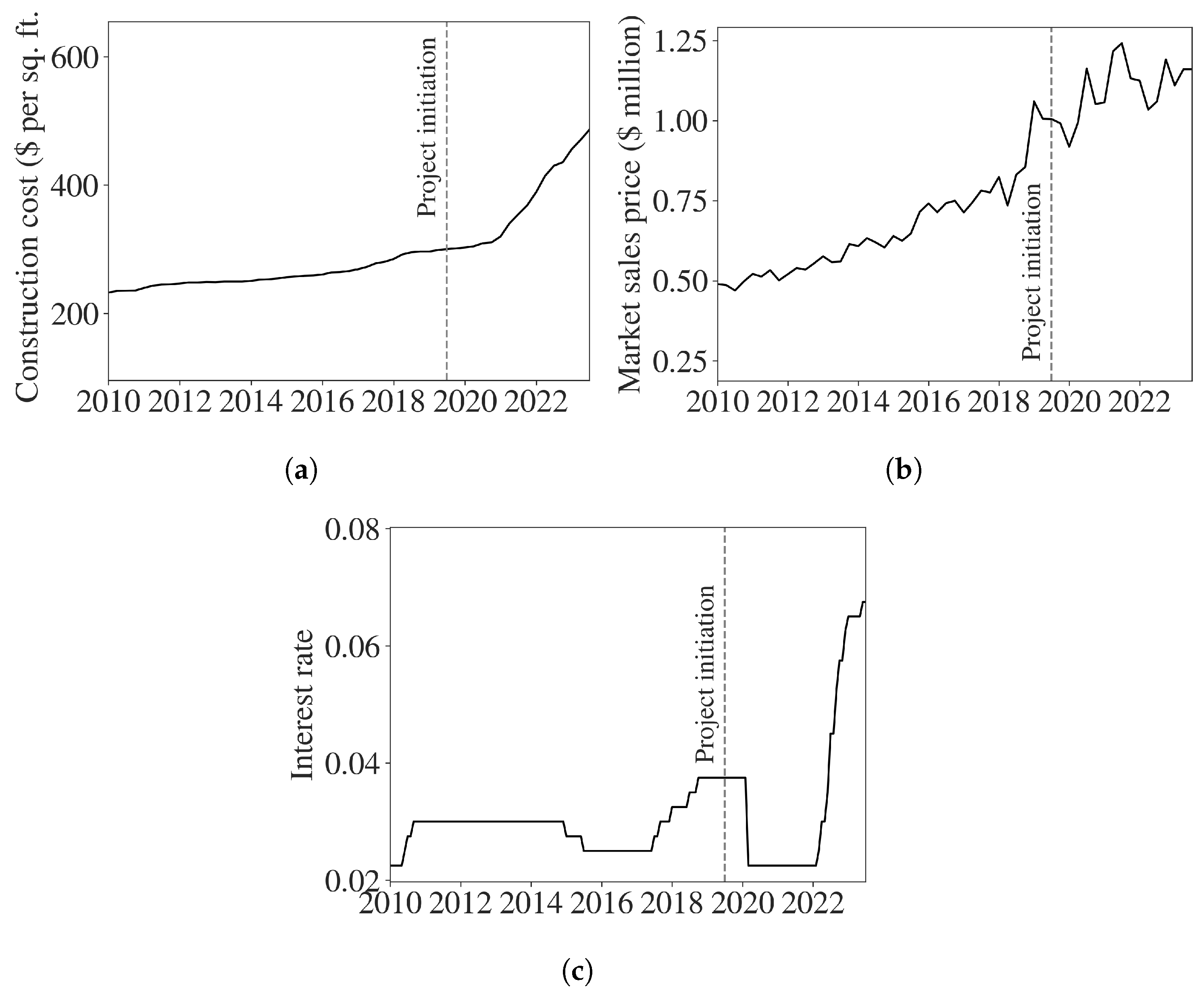
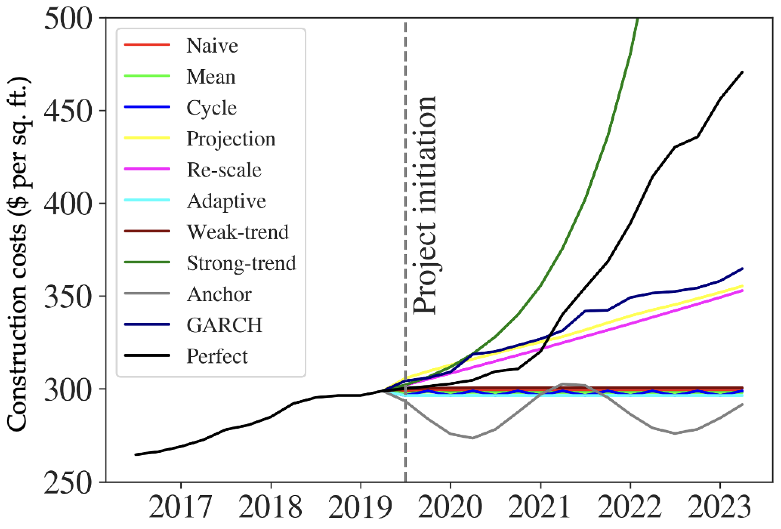
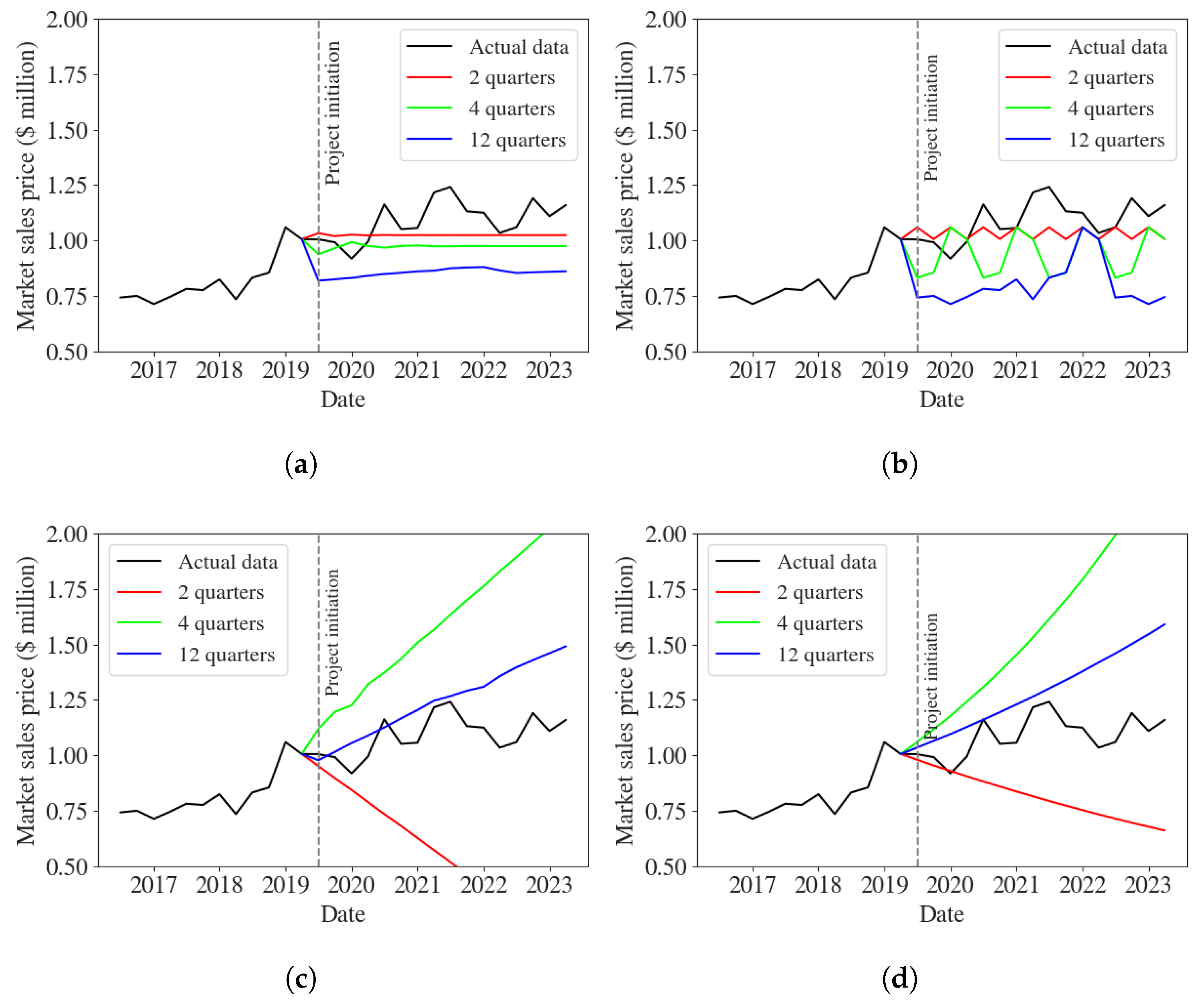
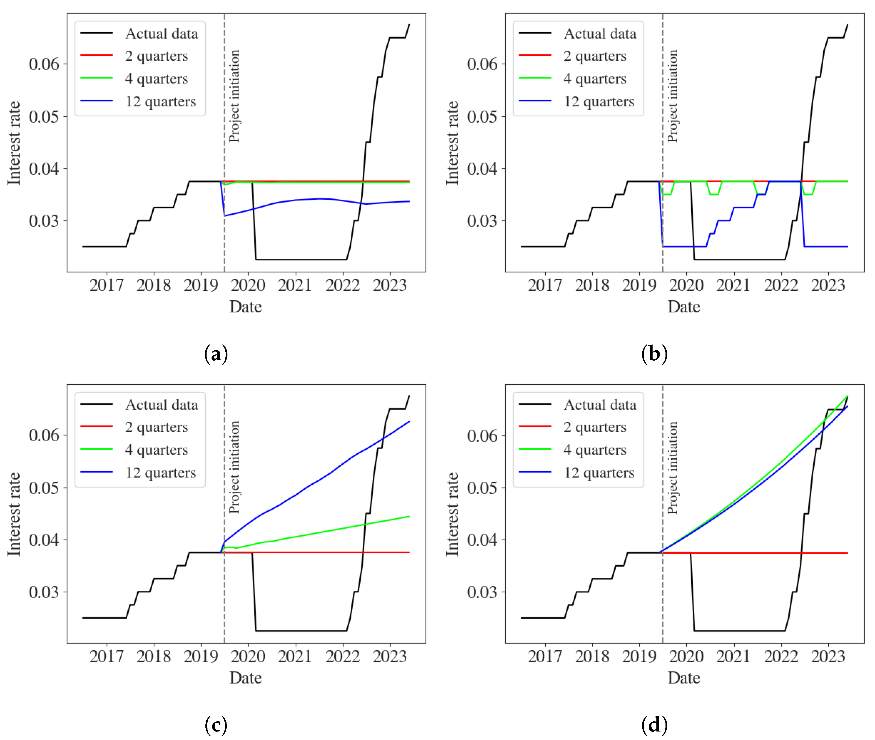
Figure 5, Figure 6 and Figure 7 represent various expectation mechanisms used at project initiation in 2019 to project construction costs, unit sales prices, and interest rates, respectively. In comparing and interpreting different expectation formation models to predict market trends, it is important to consider the characteristics and limitations of each model. While some models are simple and easy to implement, they often lack accuracy due to their simplistic assumptions. For instance, models that make less use of historical data, such as the naive model, may not capture market fluctuations, cyclical patterns, or underlying factors affecting price trends. The naive model can be basically considered the “no expectation” scenario since it assumes that future prices will remain unchanged.

The IRR estimated for our hypothetical project is demonstrated in Figure 8, considering the same boundedly rational expectation mechanisms are used at project initiation in 2019 to project construction costs, unit sales prices, and interest rates. In the examples provided in Figure 8, the IRR calculated based on the actual data, shown in black bar, represents the IRR over the lifetime of the development project given that developers could perfectly predict market trends. Therefore, this value can be used as a gauge to evaluate how each of the incorporated expectation models replicates or deviates from the actual IRR values for the project.

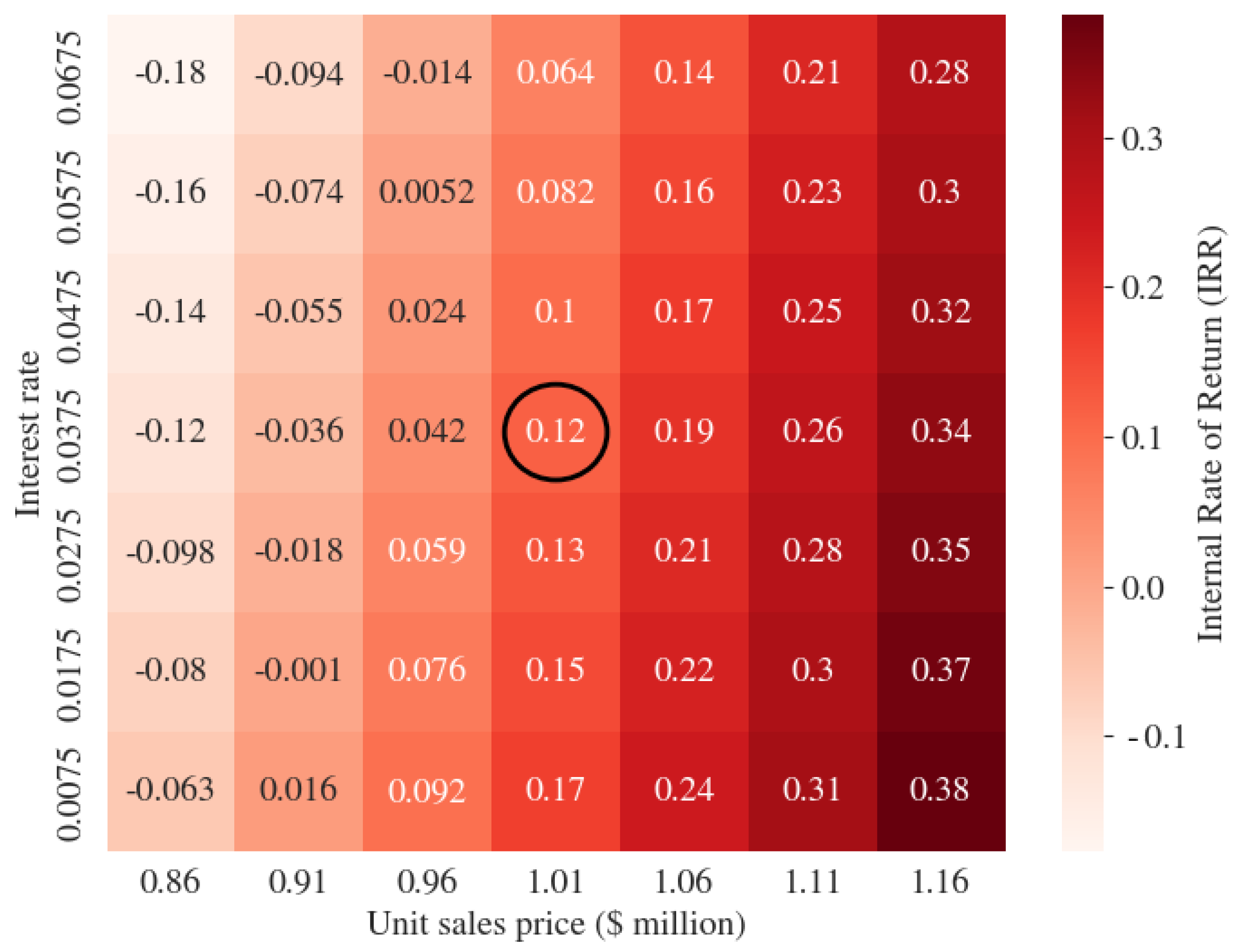
Results highlight that alternative expectation mechanisms for each of the primary factors influencing the profitability of the development project can alter the estimated IRR value. According to Figure 8, the IRR for the development project is estimated to be 12.6% using perfect expectation of construction costs, unit sales prices, and interest rates, while use of various models of expectation formations to project these trends leads to various IRR estimations at project initiation. The results suggest that boundedly rational developers who consider a MARR of 10% (the lower limit of IRR for project initiation according to key developer informants) would probably undertake the project in most cases, since the project meets their financial profitability criteria based on their perception of market trends.

As the project progresses, developers update their perception of costs and revenues based on new observation of market trends. By actively monitoring market trends, incorporating new data, and adapting their expectations, developers ensure that their financial projections remain relevant and reflective of the current market realities. This continuous updating process allows them to make more informed decisions throughout the development process and respond effectively to changing market dynamics.

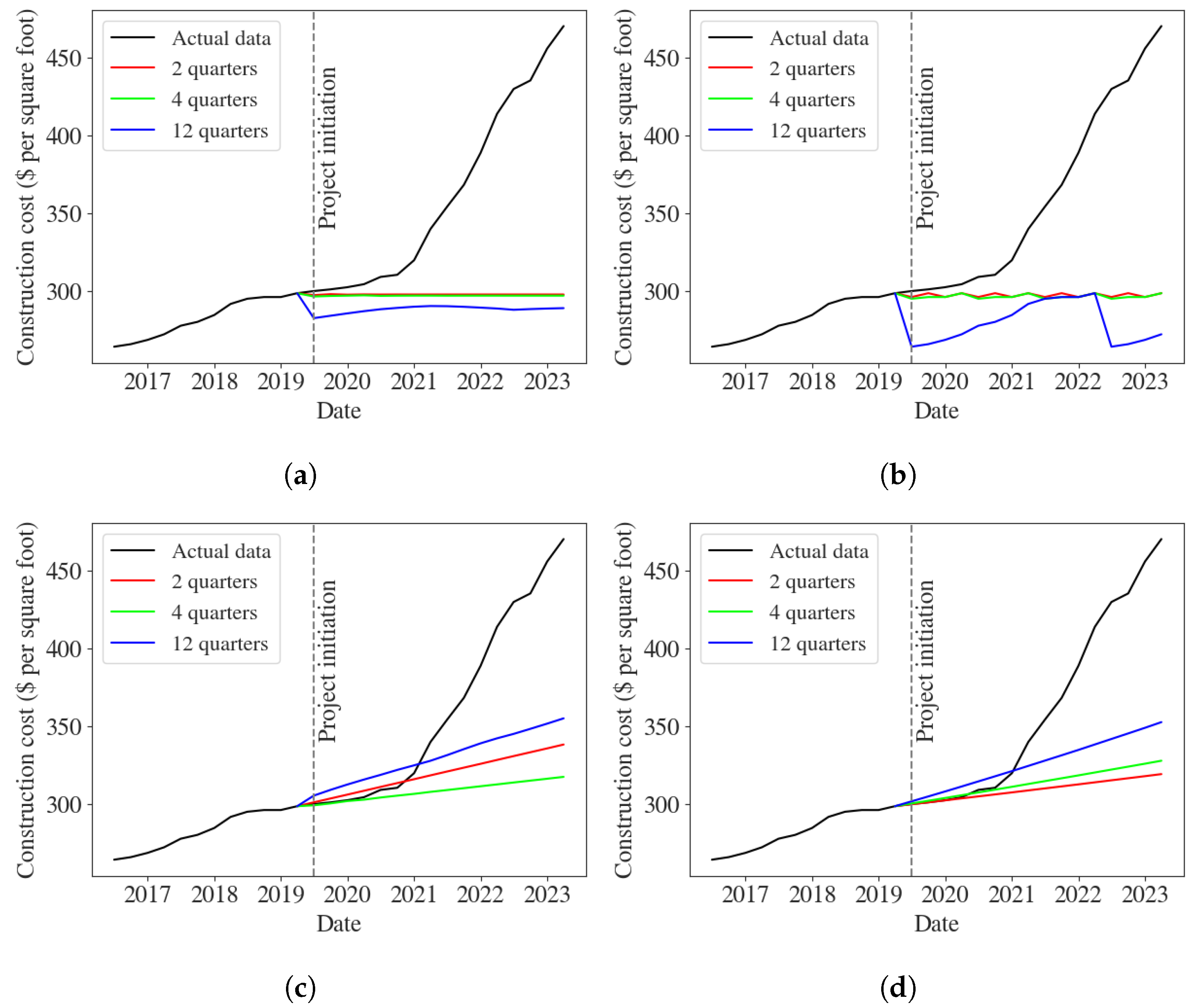
To explore how developers’ expectations of market trends during the project timeline can cause alterations in the projects, we estimated the project IRR when boundedly rational expectations are used to project construction costs, unit sales prices, and interest rates, at different times during the project. The results of this analysis are shown in Figure 9. In performing this analysis, we used the historical data prior to the decision time to reparameterize the expectation models using the same methods described in Section 3.4. This means that developers update their perceptions of market trends according to their new observations. For instance, when estimating the IRR a year after project initiation, developers use the historical data observed during the first year of the project to update their perceptions of trends for construction costs, unit sales prices, and interest rates for the rest of the project timeline.

As shown in Figure 9, use of boundedly rational expectation mechanisms to project construction costs, unit sales prices, and interest rates can lead to significant variation in the estimated IRR for the project over the project timeline. Although the initial estimation of IRR in 2019 may suggest undertaking the project, the adaptively estimated IRR for the project can significantly drop in early 2020, according to the observed decreasing trends in unit sales prices and continuously increasing construction costs. 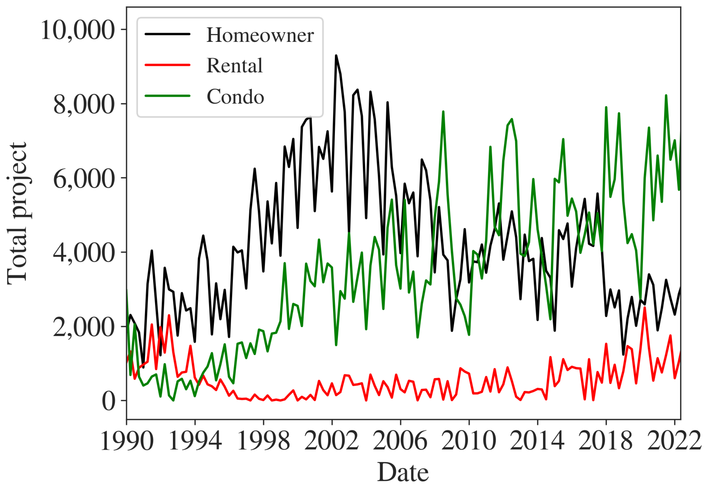According to Figure 9, after one year of project initiation in April 2020, expectation models such as the naive, the mean, the cycle, and the weak-trend estimate the project IRR at −1.63%, 1.62%, 3.42%, and −1.21%, respectively. This significant drop in the estimated IRR can put the project on pause, considering that the project is no longer expected to achieve the initially estimated financial return. These results also align with historical project cancellation trends, as shown in Figure 2, where there is an increase in the total number of project cancellations in 2020.

As time proceeds, two spikes in the project’s IRR are estimated in late 2020 and late 2021, due to decreasing interest rates and increasing unit sales prices in this period. Although the increase in construction costs has accelerated in late 2021, the results indicated that the significant increase in unit sales price during the same period could cover the extra costs imposed on the project and justify the financial feasibility of the project at this time. Observing these market trends can encourage boundedly rational developers to continue on the initiated development, hoping to achieve even higher financial returns than their initial estimations at the project start. For instance, the IRR is estimated at 33.94%, 26.55%, 33.08%, 52.01%, and 46.02% using the naive, the mean, the projection, the re-scale, and the weak-trend models, respectively. However, moving forward in the project, the estimated IRR for the project can significantly drop in 2022 and early 2023 to values below 8%, according to the rising interest rates, decreasing unit sales prices, and increasing construction costs at this period. Therefore, re-examining the financial feasibility of the project at this period can inform what adjustments in the builder’s behaviour are necessary to avoid further financial losses.

The results also indicate that adaptive expectation models that capture shifts in the market with higher accuracy can more precisely estimate the IRR values for the project. According to Figure 9, while using the naive, the mean, the cycle, and the re-scale models of expectation leads to higher variations in the IRR estimation during the project, other models that adapt to changing trends in data, such as the projection and the adaptive model, can lead to more realistic estimations of IRR during the project timeline, meaning that these models can potentially help developers make more accurate decisions. For instance, the re-scale, the weak-trend, and the anchor and adjustment models estimate the IRR to be 47.23%, 5.9%, and −1.0% at project initiation, while the projection and the adaptive models estimate the IRR to be 16.47% and 20.34%, which are closer to the actual IRR of 12.6%. Furthermore, the GARCH model failed to capture the major shift in construction cost trends and mostly overestimated the housing prices, although it captures more accurately the volatility in prices compared to other boundedly rational expectation models. The use of the GARCH model to project construction costs, unit prices, and interest rates led to an overestimation of the expected IRR by 40.3%, as the model significantly overestimated future housing prices. According to Figure 5, the GARCH model failed to capture the major shift in construction costs trends in 2020. Moreover, according to Figure 6, it mostly overestimated the housing prices since 2021, although it can more accurately capture the volatility in prices compared to other boundedly rational expectation models. However, according to Figure 9, the GARCH model can still represent the shifts in financial perceptions of housing market developers. As the project proceeds in time, recalculating the financial projections using the GARCH model for construction costs, housing prices, and interest rates, as well as also reassessing the financial viability of the projects, led to variation in the estimated IRR for the project.

5. Discussion and Conclusions

Rapid shifts in housing development costs, combined with interest rate increases resulting from recent inflationary trends in consumption goods, have significantly impacted the viability of development projects in the past few years by introducing more risks to developers’ supply decisions. Cancellation trends in condo and rental development projects can exacerbate Canada’s already severe housing shortage and further intensify its affordability crunch. Our study helps to unpack the underlying factors behind development decisions through the lens of housing market developers and understand the impact of housing market shifts on profitability perceptions and supply decisions, thus shedding light on potential solutions to our housing supply challenges.

Through formulating a sample high-rise condo proforma, we explored the primary factors influencing the profitability perceptions of housing market developers. Results highlighted that factors related to project financing and loan terms (e.g., equity funds and interest rates), property taxes, and also factors that involve a degree of uncertainty, such as construction costs and unit sales prices, can substantially influence the project revenues and costs, making them important factors in development decisions. Real-world trends in these factors have shown unexpected volatility, constituting an unexpected shock to the housing supply system.

We also explored how boundedly rational expectations of market trends can alter profitability perceptions of private developers when primary market trends (e.g., construction costs, housing prices, and interest rates) experience significant shifts, which can cause alterations in development project during the project timeline. The results suggest that boundedly rational behaviours can fail to accurately capture market trends in volatile market conditions and sometimes lead to overly optimistic projections (e.g., re-scale, trend-following, and projection models) in forecasting market trends. When relying on boundedly rational expectations, updating the profitability perceptions after project initiation can cause striking changes in the expected profit margin in unstable market conditions. This change in profitability perceptions can explain the cascade of project cancellations in the Toronto housing market, as a result of major shifts in construction costs and interest rates in the past few years.

Given the critical impact of developers on the housing market supply, paying close attention to developers’ profitability perceptions is crucial for effective policy-making in the housing market. Our findings imply that planners require a thorough understanding of development decisions and developers’ expectations, especially in volatile market conditions, to help them understand how they might best influence developer activity. This understanding can help planners encourage development decisions that align with both profit incentives and affordable housing goals through policies that can strike a balance between market dynamics and the needs of the community, such as inclusionary zoning (August and Tolfo 2018; Schuetz and Meltzer 2012) and density bonuses (Ellery 2019; Mah 2022). Our identification of high-impact factors for development profitability underscores the critical role that planners can play in shaping the financial viability of projects, when they have the agency to do so statutorily. By having a comprehensive understanding of these primary factors in development decisions, planners can transparently understand and communicate the impact of their proposed policies on potential development profitability.

Our model’s implications can vary considerably across different regions, contingent upon the prevailing policy context and market conditions. In regions marked by heightened volatility, such as those experiencing rapid price fluctuations or regulatory shifts, policy responses that directly mitigate changes in project profitability, such as the Canadian government’s recent decision to not charge sales tax for housing construction, can re-stabilize volatile markets, smoothing the housing supply (Balintec 2023). Yet, care needs to be taken to ensure that policies supports are cost-feasible for governments at all levels. In less volatile financial environments, delays in development approvals caused by planning processes, such as negotiations with city planners regarding density bonuses and inclusionary requirements, can increase uncertainty and risk for developers and their investors, potentially affecting project timelines and financial projections. Opaque zoning constraints and requirements for applications of zoning amendments can further increase uncertainty. This view supports a mandate for policymakers to formulate policies that create a more predictable environment for developers, which can contribute to a more stable and attractive investment landscape that facilitates housing supply.

While not explored in detail in this paper, the MARR reflects the perceived risk premia of developers and their investors. Feedback from local developers highlights that developers often estimate the MARR using common sense achieved through their experience from different developments, analyzing comparable projects and risk-free rates of return. It also suggests that lenders calculate risk premiums in their investment decisions to account for the risks and uncertainties associated with their decisions. Volatile market conditions often bring heightened uncertainty and unpredictability into the financial calculation and profitability estimations. Investors factor in risk premiums to mitigate potential losses stemming from unforeseen market fluctuations. These premiums could act as a financial cushion, helping to absorb losses and maintain a healthy financial position even when significant shifts impact the market (Dorofeenko et al. 2010; Trouw et al. 2020). However, a persistent increase in uncertainty and the corresponding risk premia can make a project appear less financially appealing and increase market volatility.

In modelling the financial decisions of developers, the MARR is exogenous to our model of financial profitability of potential developments, and its value is selected based input from local developers. Although understanding and modelling the effect of risk premiums on the financial decisions of lenders and developers is an important measure in investment decisions, it is beyond the focus of this paper. Nevertheless, the question of how developers and lenders formulate risk premia is an important area for future research, and would facilitate sensitivity analysis of factors that impact risk premia, such as macroeconomic volatility, construction cost fluctuations, and financial market uncertainty.

The proposed model of proforma can facilitate the incorporation of relevant uncertainties into the analysis of the profitability of potential development projects. These uncertainties stem from a lack of knowledge, especially about several input parameters of the proforma (e.g., loan interest rate and construction costs). Accounting for these uncertainties facilitates the analysis of all potential credible outcomes regarding the development project. As shown in Appendix C, incorporating relevant uncertainties can increase confidence in the model’s outputs and provide insights into the impact of uncertainties on the development decisions for developers.

Our study is motivated by a critical need for enhanced models that can better capture the real-world nuances and underlying dynamics of housing supply, which can improve the current projections of housing prices and land supply. As housing markets continually evolve, more studies are needed to improve the current projection and traditional models of land and housing prices to provide adequate capabilities that can support more reliable and evidence-based policymaking. The models presented in this study can improve the realism of actor decision models in micro-simulations/Agent-Based Models (ABMs) of land and housing markets. The review of the literature showed that few studies have incorporated price expectations into the behaviour of actors involved in land and housing markets. By more closely linking the modelled behaviours of the market actors to their real-world behaviours, the simulation dynamics will link more closely to real-world dynamics, ideally improving the simulation platforms (Sterman 2000; Valaei Sharif et al. 2023). To facilitate the replication of the proposed models, we produced Python code blocks that model the proforma and alternative expectation formation strategies, which could be utilized by any modelling team striving to represent expectation formation in agent-based market models (please refer to the Supplementary Materials for the model code). The flexible and modular design of the model facilitates the modification of the assumptions and allows for extending the model to include further details about the development projects and strategies to represent other expectation formation models.

While various expectation mechanisms representing the behaviour of housing market developers regarding estimating the market trends can lead to different outputs, the results imply that adaptive decision rules can more precisely capture the volatility and thus, predict the future trends with higher accuracy. On the other hand, models such as the naive, re-scale, trend-following, and anchor and adjustment expectations lack predictive accuracy, since they make less use of past data, leading to higher variations in predictions. The difference in the accuracy of expectation mechanisms raises a need for understanding the actual expectation formation of developers to unravel their development decisions. Understanding the actual behaviour of developers through interviews or experiments with private developers can more closely explore their decisions in unstable market conditions and help explain market volatility. Future studies can incorporate various developers’ decision strategies, drawing comparisons between different strategies and examining how actual developers’ decision strategies align with different boundedly rational models of developer decisions introduced in the literature.

References

1. Altus Group. 2022. 2022 Canadian Cost Guide. Report. Toronto: Altus Group. Available online: https://www.altusgroup.com/insights/canadian-cost-guide/ (accessed on 12 October 2023).
2. Antczak-Stępniak, Agata. 2021. Absorption rate as a tool for assessing the dynamics of development activity. Folia Oeconomica Stetinensia 21: 1–20. [Google Scholar] [CrossRef]
3. Arslan, Yavuz. 2014. Interest rate fluctuations and equilibrium in the housing market. The BE Journal of Macroeconomics 14: 173–204. [Google Scholar] [CrossRef]
4. Arthur, W. Brian. 1994. The el farol problem. American Economic Review 84: 406–11. [Google Scholar]
5. Arthur, W. Brian. 2006. Out-of-equilibrium economics and agent-based modeling. In Handbook of Computational Economics. Amsterdam: Elsevier, vol. 2, pp. 1551–1564. [Google Scholar]
6. Arthur, W. Brian. 2018. The Economy as an Evolving Complex System II. Boca Raton: CRC Press. [Google Scholar]
7. August, Martine, and Giuseppe Tolfo. 2018. Inclusionary zoning: Six insights from international experience. Plan Canada 58: 6–11. [Google Scholar] [CrossRef]
8. Axtell, Robert. 2005. The complexity of exchange. The Economic Journal 115: F193–F210. [Google Scholar] [CrossRef]
9. Balemi, Nadia, Roland Füss, and Alois Weigand. 2021. COVID-19’s impact on real estate markets: Review and outlook. Financial Markets and Portfolio Management 35: 495–513. [Google Scholar] [CrossRef]
10. Balintec, Vanessa. 2023. Could Tax Cuts Mean More Purpose-Built Rentals? Some Toronto Advocates Hope So. Newsletter article. Toronto: CBC. Available online: https://www.cbc.ca/news/canada/toronto/toronto-housing-gst-local-reaction-1.6967861 (accessed on 12 October 2023).
11. Bank of Canada. 2023. Policy Interest Rate. Website. Ottawa: Bank of Canada. Available online: https://www.bankofcanada.ca/core-functions/monetary-policy/key-interest-rate/ (accessed on 12 October 2023).
12. Banks, Jerry. 2005. Discrete Event System Simulation. Noida: Pearson Education India. [Google Scholar]
13. Bao, Te, and Cars Hommes. 2015. When Speculators Meet Constructors: Positive and Negative Feedback in Experimental Housing Markets. SOM Research Reports. Amsterdam: University of Amsterdam. [Google Scholar]
14. Barer, Justin. 2011. Mixed-Use As a Tool for Suburban Town Centre Office Space Development in Metro Vancouver: A Case Study in Port Moody, BC. Master’s thesis, Queen’s University, Kingston, ON, Canada. [Google Scholar]
15. Betts, Martin. 1991. The economic evaluation of public housing projects. Paper presented at the European Symposium on Management, Quality and Economics in Housing and Other Building Sectors, Lisbon, Portugal, September 30–October 4; Vol. 30, p. 916. [Google Scholar]
16. Bishop, Kelly C., Nicolai V. Kuminoff, Spencer Banzhaf, Kevin J. Boyle, Kathrine von Gravenitz, Jaren C. Pope, Kerry Smith, and Christopher D. Timmins. 2020. Best practices for using hedonic property value models to measure willingness to pay for environmental quality. Review of Environmental Economics and Policy 14. [Google Scholar] [CrossRef]
17. Brill, Frances. 2022. Governing investors and developers: Analysing the role of risk allocation in urban development. Urban Studies 59: 1499–517. [Google Scholar] [CrossRef]
18. Buckley, Michelle, and Glenn Brauen. 2022. Building space, building value: Residential space additions and the transformation of low-rise housing in toronto. Urban Geography 44: 1433–53. [Google Scholar]
19. Chong, Fennee. 2023. Housing price and interest rate hike: A tale of five cities in australia. Journal of Risk and Financial Management 16: 61. [Google Scholar] [CrossRef]
20. City of Toronto. 2023. Parkland Dedication. Toronto: City of Toronto. Available online: https://www.toronto.ca/city-government/planning-development/application-forms-fees/building-toronto-together-a-development-guide/parkland-dedication/ (accessed on 12 October 2023).
21. CMHC. 2022. Housing Shortages in Canada: Solving the Affordability Crisis. Report. Toronto: Canada Mortgage and Housing Corporation. Available online: https://www.cmhc-schl.gc.ca/professionals/housing-markets-data-and-research/housing-research/research-reports/accelerate-supply/housing-shortages-canada-solving-affordability-crisis (accessed on 12 October 2023).
22. CMHC. 2023a. CMHC Housing Market Information Portal. Toronto: Canada Mortgage and Housing Corporation. Available online: https://www03.cmhc-schl.gc.ca/hmip-pimh/ (accessed on 12 October 2023).
23. CMHC. 2023b. Housing Shortages in Canada: Updating How Much Housing We Need by 2030. Report. Toronto: Canada Mortgage and Housing Corporation. Available online: https://www.cmhc-schl.gc.ca/professionals/housing-markets-data-and-research/housing-research/research-reports/accelerate-supply/housing-shortages-canada-updating-how-much-we-need-by-2030 (accessed on 12 October 2023).
24. CMHC. 2023c. Starts and Completions Survey and Market Absorption Survey Methodology. Toronto: Canada Mortgage and Housing Corporation. Available online: https://www.cmhc-schl.gc.ca/professionals/housing-markets-data-and-research/housing-data/data-tables/housing-market-data (accessed on 11 October 2023).
25. Crawford, Gordon W., and Michael C. Fratantoni. 2003. Assessing the forecasting performance of regime-switching, arima and garch models of house prices. Real Estate Economics 31: 223–43. [Google Scholar] [CrossRef]
26. Cunningham, Christopher R. 2007. Growth controls, real options, and land development. The Review of Economics and Statistics 89: 343–58. [Google Scholar] [CrossRef]
27. Dorofeenko, Victor, Gabriel S. Lee, and Kevin D. Salyer. 2010. Risk Shocks and Housing Markets. Available online: https://ssrn.com/abstract=1621693 (accessed on 11 October 2023).
28. Dudley, Carlton L. 1972. A note on reinvestment assumptions in choosing between net present value and internal rate of return. The Journal of Finance 27: 907–15. [Google Scholar] [CrossRef]
29. Ellery, Randalin. 2019. Promising & Innovative Practices in Affordable Housing. Technical Report. Guelph-Wellington: Local Immigration Partnership. Available online: http://www.guelphwellingtonlip.ca/wp-content/uploads/2019/04/GWLIP-Promising-and-Innovative-Practices-in-Affordable-Housing-2019-Final-Report.pdf (accessed on 11 October 2023).
30. Engelhardt, Gary V., and James M. Poterba. 1991. House prices and demographic change: Canadian evidence. Regional Science and Urban Economics 21: 539–46. [Google Scholar] [CrossRef]
31. Ettema, Dick. 2011. A multi-agent model of urban processes: Modelling relocation processes and price setting in housing markets. Computers, Environment and Urban Systems 35: 1–11. [Google Scholar] [CrossRef]
32. Feinstein, Clarrie. 2023. 22 Percent of Canadian Homebuilders Cancel Projects Amid High Rates Despite Severe Housing Shortage. Newsletter Article. Toronto: Toronto Star. Available online: https://www.thestar.com/real-estate/22-per-cent-of-canadian-homebuilders-cancel-projects-amid-high-rates-despite-severe-housing-shortage/article_cbcccf90-2426-599b-8c11-3d42c45382f4.html (accessed on 11 October 2023).
33. Felsenstein, Daniel, and Eyal Ashbel. 2010. Simultaneous modeling of developer behavior and land prices in urbansim. Journal of Transport and Land Use 3: 107–27. [Google Scholar] [CrossRef]
34. Filatova, Tatiana. 2015. Empirical agent-based land market: Integrating adaptive economic behavior in urban land-use models. Computers, Environment and Urban Systems 54: 397–413. [Google Scholar] [CrossRef]
35. Filatova, Tatiana, Dawn Cassandra Parker, and Anne Van der Veen. 2009. Agent-based urban land markets: Agent’s pricing behavior, land prices and urban land use change. Journal of Artificial Societies and Social Simulation 12: 3. [Google Scholar]
36. Finnegan, Marshall. 2023. Purpose-Built Rental Housing in the Greater Toronto Area. Technical Report. Toronto: Building Industry and Land Development Association. Available online: https://www.bildgta.ca/wp-content/uploads/2023/02/Purpose-Built-Rental-Whitepaper-FINAL.pdf (accessed on 11 October 2023).
37. Fox, Chris. 2022. Developers Could Cancel about 5,000 New Condo Units as Construction Prices Rise, Industry Observer Says. Newsletter Article. Toronto: CP24. Available online: https://www.cp24.com/news/developers-could-cancel-approximately-5-000-new-condo-units-as-construction-prices-rise-industry-observer-says-1.5956607 (accessed on 11 October 2023).
38. Fraser, Niall M., and Elizabeth M. Jewkes. 2012. Engineering Economics: Financial Decision Making for Engineers. North York: Pearson Education Canada. [Google Scholar]
39. Gilbert, Nigel, John C. Hawksworth, and Paul A. Swinney. 2009. An agent-based model of the english housing market. In AAAI Spring Symposium: Technosocial Predictive Analytics. Washington, DC: Association for the Advancement of Artificial Intelligence, pp. 30–35. [Google Scholar]
40. Gong, Yifan, and Yuxi Yao. 2022. Demographic changes and the housing market. Regional Science and Urban Economics 95: 103734. [Google Scholar] [CrossRef]
41. Hollander, Justin B., and Nicole E. Stephens. 2023. Buildings for People: Responsible Real Estate Development and Planning. Hoboken: Wiley. [Google Scholar]
42. Hommes, Cars. 2021. Behavioral and experimental macroeconomics and policy analysis: A complex systems approach. Journal of Economic Literature 59: 149–219. [Google Scholar] [CrossRef]
43. Hommes, Cars, Joep Sonnemans, Jan Tuinstra, and Henk van de Velden. 2005. A strategy experiment in dynamic asset pricing. Journal of Economic Dynamics and Control 29: 823–43. [Google Scholar] [CrossRef]
44. Ho, Winky K. O., Bo-Sin Tang, and Siu Wai Wong. 2021. Predicting property prices with machine learning algorithms. Journal of Property Research 38: 48–70. [Google Scholar] [CrossRef]
45. Huang, Yu. 2020. Analyzing Housing Market Dynamics and Residential Location Choices Concurrent with Light-Rail Transit Investment in Kitchener-Waterloo, Canada. Ph.D. thesis, University of Waterloo, Waterloo, ON, Canada. Available online: http://hdl.handle.net/10012/15801 (accessed on 11 October 2023).
46. Huang, Yu, Dawn Cassandra Parker, and Leia Minaker. 2021. Identifying latent demand for transit-oriented development neighbourhoods: Evidence from a mid-sized urban area in canada. Journal of Transport Geography 90: 102940. [Google Scholar] [CrossRef]
47. Hunt, John D., David S. Kriger, and Eric J. Miller. 2005. Current operational urban land-use–transport modelling frameworks: A review. Transport Reviews 25: 329–76. [Google Scholar] [CrossRef]
48. Imrie, Rob, and Emma Street. 2009. Risk, regulation and the practices of architects. Urban Studies 46: 2555–76. [Google Scholar] [CrossRef]
49. Jeanty, P. Wilner, Mark Partridge, and Elena Irwin. 2010. Estimation of a spatial simultaneous equation model of population migration and housing price dynamics. Regional Science and Urban Economics 40: 343–52. [Google Scholar] [CrossRef]
50. Jennings, Will. 2012. Why costs overrun: Risk, optimism and uncertainty in budgeting for the london 2012 olympic games. Construction Management and Economics 30: 455–62. [Google Scholar] [CrossRef]
51. Johnson, Jerry, Jeff Frkonja, Maribeth Todd, and Dennis Yee. 2018. Additional detail in aggregate integrated land-use models via simulating developer pro forma thinking. Journal of Transport and Land Use 11: 405–18. [Google Scholar] [CrossRef]
52. Justiniano, Alejandro, Giorgio E. Primiceri, and Andrea Tambalotti. 2019. Credit supply and the housing boom. Journal of Political Economy 127: 1317–50. [Google Scholar] [CrossRef]
53. Kashani, Hamed, Shahab Valaei Sharif, Shiva Hosseini, and Mohamad Ali Hekmatian. 2022. Dynamical modeling of outbreak and control of pandemics: Assessing the resilience of healthcare infrastructure under mitigation policies. In The Science behind the COVID Pandemic and Healthcare Technology Solutions. Berlin/Heidelberg: Springer, pp. 329–51. [Google Scholar]
54. Koo, ChoongWan, TaeHoon Hong, and ChangTaek Hyun. 2011. The development of a construction cost prediction model with improved prediction capacity using the advanced cbr approach. Expert Systems with Applications 38: 8597–606. [Google Scholar] [CrossRef]
55. Kuchler, Theresa, Monika Piazzesi, and Johannes Stroebel. 2023. Housing market expectations. In Handbook of Economic Expectations. Amsterdam: Elsevier, pp. 163–91. [Google Scholar]
56. Lee, Chyi Lin, and Richard G. Reed. 2014. The relationship between housing market intervention for first-time buyers and house price volatility. Housing Studies 29: 1073–95. [Google Scholar] [CrossRef]
57. Lehrer, Ute, Roger Keil, and Stefan Kipfer. 2010. Reurbanization in toronto: Condominium boom and social housing revitalization. DisP-The Planning Review 46: 81–90. [Google Scholar] [CrossRef]
58. Leung, Andrew Y. T., Jia-na Xu, and Wing Shum Tsui. 2009. A heterogeneous boundedly rational expectation model for housing market. Applied Mathematics and Mechanics 30: 1305–16. [Google Scholar] [CrossRef]
59. Liu, Tian, Weiyan Hu, Yan Song, and Anlu Zhang. 2020. Exploring spillover effects of ecological lands: A spatial multilevel hedonic price model of the housing market in Wuhan, China. Ecological Economics 170: 106568. [Google Scholar] [CrossRef]
60. Lorga, Miguel, João Fragoso Januário, and Carlos Oliveira Cruz. 2022. Housing affordability, public policy and economic dynamics: An analysis of the city of lisbon. Journal of Risk and Financial Management 15: 560. [Google Scholar] [CrossRef]
61. Magliocca, Nicholas, Elena Safirova, Virginia McConnell, and Margaret Walls. 2011. An economic agent-based model of coupled housing and land markets (chalms). Computers, Environment and Urban Systems 35: 183–91. [Google Scholar] [CrossRef]
62. Magliocca, Nicholas R., Daniel G. Brown, and Erle C. Ellis. 2014a. Cross-site comparison of land-use decision-making and its consequences across land systems with a generalized agent-based model. PLoS ONE 9: e86179. [Google Scholar] [CrossRef]
63. Magliocca, Nicholas R., Daniel G. Brown, Virginia D. McConnell, Joan I. Nassauer, and Westbrook Elizabeth. 2014b. Effects of alternative developer decision-making models on the production of ecological subdivision designs: Experimental results from an agent-based model. Environment and Planning B: Planning and Design 41: 907–27. [Google Scholar] [CrossRef]
64. Mah, Julie. 2022. Evaluating Affordable Housing Outcomes in Toronto: An Analysis of Density Bonusing Agreements. Toronto: Institute on Municipal Finance and Governance. [Google Scholar]
65. Martin, Carolin, Noemi Schmitt, and Frank Westerhoff. 2021. Heterogeneous expectations, housing bubbles and tax policy. Journal of Economic Behavior & Organization 183: 555–73. [Google Scholar] [CrossRef]
66. Maruani, Tseira, and Irit Amit-Cohen. 2011. Characteristics of developers and their relations to open space conservation. Land Use Policy 28: 887–97. [Google Scholar] [CrossRef]
67. Mohamed, Rayman. 2006. The psychology of residential developers: Lessons from behavioral economics and additional explanations for satisficing. Journal of Planning Education and Research 26: 28–37. [Google Scholar] [CrossRef]
68. Murray, Cameron K. 2022. A housing supply absorption rate equation. The Journal of Real Estate Finance and Economics 64: 228–46. [Google Scholar] [CrossRef]
69. Nguyen-Luong, Dany. 2008. An Integrated Land Use-Transport Model for the Paris Region (simaurif): Ten Lessons Learned after Four Years of Development. Technical Report. Documento de trabalho-Institut d’aménagement et d’urbanisme de la région Ile-de-France-IAURIF (não publicado). Available online: https://web.mit.edu/11.521/proj08/readings/D_Mes_documentsDNLpredit3ERSA_2008article_SIMAURIF_10_lessons.pdf (accessed on 11 October 2023).
70. Okwilagwe, Osikhuemhe, and Christos Apostolakis. 2017. Implementation of Partnership Work: Key Considerations and Implications from the Nigerian Local Regeneration. Technical Report. Poole: Bournemouth University. Available online: https://eprints.bournemouth.ac.uk/33809/ (accessed on 11 October 2023).
71. Pai, Ping-Feng, and Wen-Chang Wang. 2020. Using machine learning models and actual transaction data for predicting real estate prices. Applied Sciences 10: 5832. [Google Scholar] [CrossRef]
72. Parker, Dawn Cassandra, and Tatiana Filatova. 2008. A conceptual design for a bilateral agent-based land market with heterogeneous economic agents. Computers, Environment and Urban Systems 32: 454–63. [Google Scholar] [CrossRef]
73. Parker, Dawn Cassandra, Shahab Valaei Sharif, and Kaitlin Webber. 2023. Why did the “missing middle” miss the train? An actors-in-systems exploration of barriers to intensified family housing in Waterloo region, Canada. Land 12: 434. [Google Scholar] [CrossRef]
74. Paull, Hermina. 2022. Toronto’s Condo Oversupply Gives Buyers, Renters More Negotiating Power. Newsletter Article. Canada: The Deep Dive. Available online: https://thedeepdive.ca/torontos-condo-oversupply-gives-buyers-renters-more-negotiating-power/ (accessed on 11 October 2023).
75. Salvati, Luca, Maria Teresa Ciommi, Pere Serra, and Francesco M Chelli. 2019. Exploring the spatial structure of housing prices under economic expansion and stagnation: The role of socio-demographic factors in metropolitan Rome, Italy. Land Use Policy 81: 143–52. [Google Scholar] [CrossRef]
76. Sarnoff, Nancy. 2022. Toronto Claims It Wants More Missing Middle Housing, So Why Isn’t It Making It Easier to Build. Newsletter article. Toronto: Storeys. Available online: https://storeys.com/toronto-more-missing-middle-housing-why-make-hard-to-build/ (accessed on 11 October 2023).
77. Schuetz, Jenny, and Rachel Meltzer. 2012. Inclusionary zoning to support affordable housing. International Encyclopedia of Housing and Home, 32–36. [Google Scholar] [CrossRef]
78. Sherman, Josh. 2022. Toronto’s Housing Shortage Takes a Turn for the Worse as Developers Cancel Projects. Newsletter Article. Toronto: Streets of Toronto. Available online: https://streetsoftoronto.com/toronto-housing-shortage-worsens-with-developers-cancelling-new-projects/ (accessed on 11 October 2023).
79. Silva, Elisabete A. 2002. Indecision factors when planning for land use change. European Planning Studies 10: 335–58. [Google Scholar] [CrossRef]
80. Smyth, Hedley. 2005. Trust in the design team. Architectural Engineering and Design Management 1: 211–23. [Google Scholar] [CrossRef]
81. Statistics Canada. 2023. Building construction price indexes, percentage change, quarterly, inactive. Statistics Canada. [Google Scholar] [CrossRef]
82. Sterman, John. 2000. Business Dynamics. New York: McGraw-Hill, Inc. [Google Scholar]
83. Sutton, Gregory D., Dubravko Mihaljek, and Agne Subelyte. 2017. Interest Rates and House Prices in the United States and Around the World. Report. Basel: Bank for International Settlements. Available online: https://www.bis.org/publ/work665.pdf (accessed on 11 October 2023).
84. Taltavull, Paloma, and Stanley McGreal. 2009. Measuring price expectations: Evidence from the spanish housing market. Journal of European Real Estate Research 2: 186–209. [Google Scholar] [CrossRef]
85. Trouw, Michael, Stephan Weiler, and Jesse Silverstein. 2020. Brownfield development: Uncertainty, asymmetric information, and risk premia. Sustainability 12: 2046. [Google Scholar] [CrossRef]
86. Urbanation. 2023. Condo Project and Unit Cancellations in the Greater Toronto Area (GTA). Database. Toronto: Urbanation. Available online: https://www.urbanation.ca (accessed on 11 October 2023).
87. Valaei Sharif, Shahab, Peyman Habibi Moshfegh, and Hamed Kashani. 2023. Simulation modeling of operation and coordination of agencies involved in post-disaster response and recovery. Reliability Engineering & System Safety 235: 109219. [Google Scholar]
88. Valaei Sharif, Shahab, Peyman Habibi Moshfegh, Mohamad Ali Morshedi, and Hamed Kashani. 2022. Modeling the impact of mitigation policies in a pandemic: A system dynamics approach. International Journal of Disaster Risk Reduction 82: 103327. [Google Scholar] [CrossRef]
89. Wagner, Peter, and Michael Wegener. 2007. Urban land use, transport and environment models: Experiences with an integrated microscopic approach. DisP-The Planning Review 43: 45–56. [Google Scholar] [CrossRef]
90. Wegener, Michael. 2021. Land-use transport interaction models. In Handbook of Regional Science. Berlin/Heidelberg: Springer, pp. 229–46. [Google Scholar]
91. White, John A., Kellie S. Grasman, Kenneth E. Case, Kim LaScola Needy, and David B. Pratt. 2020. Fundamentals of Engineering Economic Analysis. Hoboken: John Wiley & Sons. [Google Scholar]
92. Winarso, Haryo. 2000. Developer’s Behaviour in Residential Land Development in Jabothek, Indonesia. Ph.D. thesis, University of London, London, UK. [Google Scholar]
93. Wood, Gerard D., and Robert C. T. Ellis. 2003. Risk management practices of leading uk cost consultants. Engineering, Construction and Architectural Management 10: 254–62. [Google Scholar] [CrossRef]
94. Yang, Linchuan, Kwong W. Chau, Wai Y. Szeto, Xu Cui, and Xu Wang. 2020a. Accessibility to transit, by transit, and property prices: Spatially varying relationships. Transportation Research Part D: Transport and Environment 85: 102387. [Google Scholar] [CrossRef]
95. Yang, Linchuan, Xiaoling Chu, Zhonghua Gou, Hongtai Yang, Yi Lu, and Wencheng Huang. 2020b. Accessibility and proximity effects of bus rapid transit on housing prices: Heterogeneity across price quantiles and space. Journal of Transport Geography 88: 102850. [Google Scholar] [CrossRef]
96. Younglai, Rachelle. 2022. Toronto Could Face Wave of Condo Project Cancellations as Costs Rise. Newsletter article. Toronto: The Globe and Mail. Available online: https://www.theglobeandmail.com/business/article-toronto-could-face-wave-of-condo-project-cancellations-as-costs-rise/ (accessed on 11 October 2023).
Figure 1. Historical development project starts by the intended market in Toronto (CMHC 2023c).
Jrfm 16 00446 g001
Figure 2. Historical condo project cancellations in the GTA land and housing market by Urbanation (2023): (a) total number of projects and (b) total number of units.
Jrfm 16 00446 g002
Figure 3. Impact of increase in interest rates on the development decisions through decreasing unit sales prices and increasing finance costs. Signs show the direction of change: a positive sign represents an increase and a negative sign denotes a decrease.
Jrfm 16 00446 g003
Figure 4. Historical market trends for (a) construction costs (Altus Group 2022; Statistics Canada 2023), (b) sales prices of properties (CMHC 2023a), and (c) loan interest rates estimated as the prime interest rate plus 2% (Bank of Canada 2023) in the Toronto land and housing markets.
Jrfm 16 00446 g004
Figure 5. Parameterized expectation models at project initiation in 2019 to predict the market trends for construction costs during the project until 2023.
Jrfm 16 00446 g005
Figure 6. Parameterized expectation models at project initiation in 2019 to predict the market trends for unit sales prices during the project until 2023.
Jrfm 16 00446 g006
Figure 7. Parameterized expectation models at project initiation in 2019 to predict the market trends for interest rates during the project until 2023.
Jrfm 16 00446 g007
Figure 8. Estimated IRR for the development project when considering the same expectation mechanisms to project construction costs, unit sales prices, and loan interest rate.
Jrfm 16 00446 g008
Figure 9. Estimated IRR for the project at different times during the project when the same boundedly rational expectation mechanisms are used to project construction costs, unit sales prices, and interest rates.
Jrfm 16 00446 g009