
Forecasting of NIFTY 50 Index Price by Using Backward Elimination with an LSTM Model

 ,
,  ,
,  , and
, and
Abstract
:1. Introduction
2. Related Work
3. Methodology
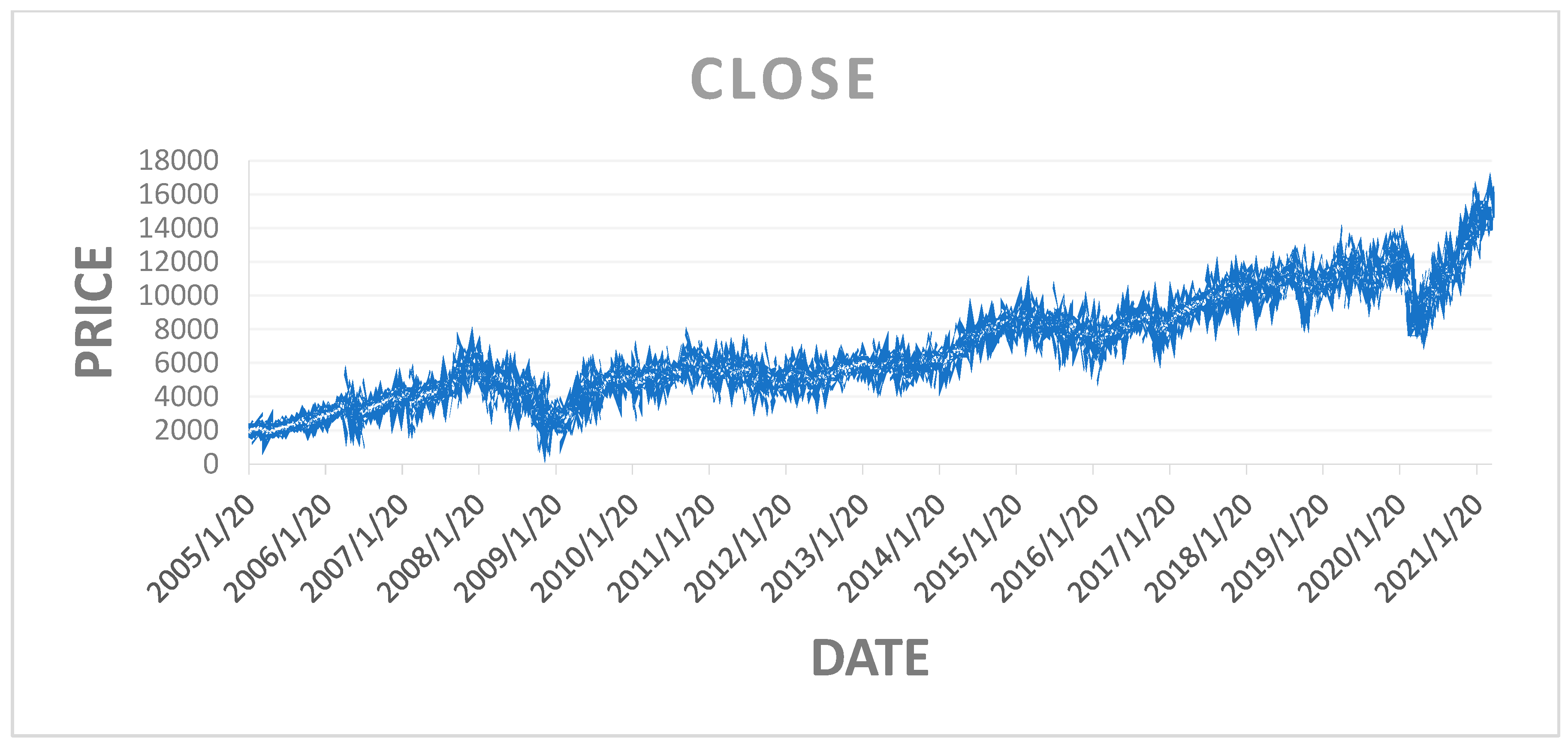
3.1. Data Collection
3.2. Data Pre-Processing
- Step 1. Formulate the Hypotheses:
- Null hypothesis (H0): The proportions are equal; S = S0.
- Alternative hypothesis (H1): The proportions are not equal; S # S0.
- Step 2. Calculate the Sample Proportions:
- S is the proportion of success in the sample.
- S0 is the hypothesized proportion of success (given in the null hypothesis).
- Step 3. Calculate the Standard Error:
- Step 4. Calculate the Z-score:
- Step 5. Determine the Critical Value or p-value:
- Step 6. Make a Decision:
- Step 7. Interpretation:
3.3. LSTM Model
3.4. Backward Elimination with LSTM (BE-LSTM)
3.5. Evaluation Metrics
- Accuracy
- Precision
- The model produces a substantial number of correct positive classifications, thus maximising the true positives.
- The model minimizes the number of incorrect positive classifications, thereby reducing false positives.
- Recall
4. Results and Discussion
5. Conclusions and Future Scope
Author Contributions
Funding
Institutional Review Board Statement
Informed Consent Statement
Data Availability Statement
Conflicts of Interest
References
- Abraham, Rebecca, Mahmoud El Samad, Amer M. Bakhach, Hani El-Chaarani, Ahmad Sardouk, Sam El Nemar, and Dalia Jaber. 2022. Forecasting a Stock Trend Using Genetic Algorithm and Random Forest. Journal of Risk and Financial Management 5: 188. [Google Scholar] [CrossRef]
- Ananthi, M., and K. Vijayakumar. 2021. Stock market analysis using candlestick regression and market trend prediction (CKRM). Journal of Ambient Intelligence and Humanized Computing 12: 4819–26. [Google Scholar] [CrossRef]
- Ariyo, Adebiyi A., Adewumi O. Adewumi, and Charles K. Ayo. 2014. Stock price prediction using the ARIMA model. Paper presented at 2014 UKSim-AMSS 16th International Conference on Computer Modelling and Simulation, Cambridge, UK, March 26–28. [Google Scholar]
- Asghar, Muhammad Zubair, Fazal Rahman, Fazal Masud Kundi, and Shakeel Ahmad. 2019. Development of stock market trend prediction system using multiple regression. Computational and Mathematical Organization Theory 25: 271–301. [Google Scholar] [CrossRef]
- Bathla, Gourav, Rinkle Rani, and Himanshu Aggarwal. 2023. Stocks of year 2020: Prediction of high variations in stock prices using LSTM. Multimedia Tools and Applications 7: 9727–43. [Google Scholar] [CrossRef]
- Chen, Wei, Haoyu Zhang, Mukesh Kumar Mehlawat, and Lifen Jia. 2021. Mean-variance portfolio optimization using machine learning-based stock price prediction. Applied Soft Computing 100: 106943. [Google Scholar] [CrossRef]
- Cui, Tianxiang, Shusheng Ding, Huan Jin, and Yongmin Zhang. 2023. Portfolio constructions in cryptocurrency market: A CVaR-based deep reinforcement learning approach. Economic Modelling 119: 106078. [Google Scholar] [CrossRef]
- Dash, Rajashree, Sidharth Samal, Rasmita Dash, and Rasmita Rautray. 2019. An integrated TOPSIS crow search based classifier ensemble: In application to stock index price movement prediction. Applied Soft Computing 85: 105784. [Google Scholar] [CrossRef]
- El-Chaarani, Hani. 2019. The Impact of Oil Prices on Stocks Markets: New Evidence During and After the Arab Spring in Gulf Cooperation Council Economies. International Journal of Energy Economics and Policy 9: 214–223. [Google Scholar] [CrossRef]
- Gao, Ruize, Xin Zhang, Hongwu Zhang, Quanwu Zhao, and Yu Wang. 2022. Forecasting the overnight return direction of stock market index combining global market indices: A multiple-branch deep learning approach. Expert Systems with Applications 194: 116506. [Google Scholar] [CrossRef]
- Idrees, Sheikh Mohammad, M. Afshar Alam, and Parul Agarwal. 2019. A prediction approach for stock market volatility based on time series data. IEEE Access 7: 17287–98. [Google Scholar] [CrossRef]
- Ilkka, Virtanen, and Paavo Yli-Olli. 1987. Forcasting stock market prices in a thin security market. Omega 15: 145–55. [Google Scholar]
- Jain, Vikalp Ravi, Manisha Gupta, and Raj Mohan Singh. 2018. Analysis and prediction of individual stock prices of financial sector companies in NIFTY 50. International Journal of Information Engineering and Electronic Business 2: 33–41. [Google Scholar] [CrossRef]
- Jiang, Weiwei. 2021. Applications of deep learning in stock market prediction: Recent progress. Expert Systems with Applications 184: 115537. [Google Scholar] [CrossRef]
- Jin, Guangxun, and Ohbyung Kwon. 2021. Impact of chart image characteristics on stock price prediction with a convolutional neural network. PLoS ONE 16: e0253121. [Google Scholar] [CrossRef]
- Jing, Nan, Zhao Wu, and Hefei Wang. 2021. A hybrid model integrating deep learning with investor sentiment analysis for stock price prediction. Expert Systems with Applications 178: 115019. [Google Scholar] [CrossRef]
- Khaidem, Luckyson, Snehanshu Saha, and Sudeepa Roy Dey. 2016. Predicting the direction of stock market prices using random forest. arXiv arXiv:1605.00003. [Google Scholar]
- Kurani, Akshit, Pavan Doshi, Aarya Vakharia, and Manan Shah. 2023. A comprehensive comparative study of artificial neural network (ANN) and support vector machines (SVM) on stock forecasting. Annals of Data Science 10: 183–208. [Google Scholar] [CrossRef]
- Liu, Keyan, Jianan Zhou, and Dayong Dong. 2021. Improving stock price prediction using the long short-term memory model combined with online social networks. Journal of Behavioral and Experimental Finance 30: 100507. [Google Scholar] [CrossRef]
- Long, Wen, Zhichen Lu, and Lingxiao Cui. 2019. Deep learning-based feature engineering for stock price movement prediction. Knowledge-Based Systems 164: 163–73. [Google Scholar] [CrossRef]
- Mahajan, Vanshu, Sunil Thakan, and Aashish Malik. 2022. Modeling and forecasting the volatility of NIFTY 50 using GARCH and RNN models. Economies 5: 102. [Google Scholar] [CrossRef]
- Mahboob, Khalid, Muhammad Huzaifa Shahbaz, Fayyaz Ali, and Rohail Qamar. 2023. Predicting the Karachi Stock Price index with an Enhanced multi-layered Sequential Stacked Long-Short-Term Memory Model. VFAST Transactions on Software Engineering 2: 249–55. [Google Scholar]
- Maniatopoulos, Andreas-Antonios, Alexandros Gazis, and Nikolaos Mitianoudis. 2023. Technical analysis forecasting and evaluation of stock markets: The probabilistic recovery neural network approach. International Journal of Economics and Business Research 1: 64–100. [Google Scholar] [CrossRef]
- Mehtab, Sidra, and Jaydip Sen. 2020. Stock price prediction using convolutional neural networks on a multivariate time series. arXiv arXiv:2001.09769. [Google Scholar]
- Mehtab, Sidra, Jaydip Sen, and Abhishek Dutta. 2020. Stock price prediction using machine learning and LSTM-based deep learning models. In Symposium on Machine Learning and Metaheuristics Algorithms, and Applications. Singapore: Springer, pp. 88–106. [Google Scholar]
- Mondal, Bhaskar, Om Patra, Ashutosh Satapathy, and Soumya Ranjan Behera. 2021. A Comparative Study on Financial Market Forecasting Using AI: A Case Study on NIFTY. In Emerging Technologies in Data Mining and Information Security. Singapore: Springer, vol. 1286, pp. 95–103. [Google Scholar]
- Nelson, David M. Q., Adriano C. M. Pereira, and Renato A. de Oliveira. 2017. Stock market’s price movement prediction with LSTM neural networks. Paper presented at 2017 International Joint Conference on Neural Networks (IJCNN), Anchorage, AK, USA, May 14–19; New York: IEEE, pp. 1419–26. [Google Scholar]
- Olorunnimbe, Kenniy, and Herna Viktor. 2023. Deep learning in the stock market—A systematic survey of practice, backtesting, and applications. Artificial Intelligence Review 56: 2057–109. [Google Scholar] [CrossRef]
- Ostermark, R. 1989. Predictability of finnish and Swedish stock returns. Omega 17: 223–36. [Google Scholar] [CrossRef]
- Oukhouya, Hassan, and Khalid El Himdi. 2023. Comparing Machine Learning Methods—SVR, XGBoost, LSTM, and MLP—For Forecasting the Moroccan Stock Market. Computer Sciences and Mathematics Forum 1: 39. [Google Scholar]
- Parmar, Ishita, Navanshu Agarwal, Sheirsh Saxena, Ridam Arora, Shikhin Gupta, Himanshu Dhiman, and Lokesh Chouhan. 2018. Stock market prediction using machine learning. Paper presented at 2018 First International Conference on Secure Cyber Computing and Communication (ICSCCC), Jalandhar, India, December 15–17; New York: IEEE, pp. 574–76. [Google Scholar]
- Polamuri, Subba Rao, Kudipudi Srinivas, and A. Krishna Mohan. 2021. Multi-Model Generative Adversarial Network Hybrid Prediction Algorithm (MMGAN-HPA) for stock market prices prediction. Journal of King Saud University-Computer and Information Sciences 9: 7433–44. [Google Scholar] [CrossRef]
- Rezaei, Hadi, Hamidreza Faaljou, and Gholamreza Mansourfar. 2021. Stock price prediction using deep learning and frequency decomposition. Expert Systems with Applications 169: 114332. [Google Scholar] [CrossRef]
- Ribeiro, Gabriel Trierweiler, André Alves Portela Santos, Viviana Cocco Mariani, and Leandro dos Santos Coelho. 2021. Novel hybrid model based on echo state neural network applied to the prediction of stock price return volatility. Expert Systems with Applications 184: 115490. [Google Scholar] [CrossRef]
- Sarode, Sumeet, Harsha G. Tolani, Prateek Kak, and C. S. Lifna. 2019. Stock price prediction using machine learning techniques. Paper presented at 2019 International Conference on Intelligent Sustainable Systems (ICISS), Palladam, India, February 21–22; New York: IEEE, pp. 177–81. [Google Scholar]
- Selvamuthu, Dharmaraja, Vineet Kumar, and Abhishek Mishra. 2019. Indian stock market prediction using artificial neural networks on tick data. Financial Innovation 5: 16. [Google Scholar] [CrossRef]
- Sezer, Omer Berat, Mehmet Ugur Gudelek, and Ahmet Murat Ozbayoglu. 2020. Financial time series forecasting with deep learning: A systematic literature review: 2005–19. Applied Soft Computing 90: 106181. [Google Scholar] [CrossRef]
- Sharma, Dhruv, Amisha, Pradeepta Kumar Sarangi, and Ashok Kumar Sahoo. 2023. Analyzing the Effectiveness of Machine Learning Models in Nifty50 Next Day Prediction: A Comparative Analysis. Paper presented at 2023 3rd International Conference on Advance Computing and Innovative Technologies in Engineering (ICACITE), Noida, India, May 12–13; New York: IEEE, pp. 245–50. [Google Scholar]
- Shen, Jingyi, and M. Omair Shafiq. 2020. Short-term stock market price trend prediction using a comprehensive deep learning system. Journal of Big Data 7: 1–33. [Google Scholar] [CrossRef]
- Sheth, Dhruhi, and Manan Shah. 2023. Predicting stock market using machine learning: Best and accurate way to know future stock prices. International Journal of System Assurance Engineering and Management 14: 1–18. [Google Scholar] [CrossRef]
- Sisodia, Pushpendra Singh, Anish Gupta, Yogesh Kumar, and Gaurav Kumar Ameta. 2022. Stock market analysis and prediction for NIFTY50 using LSTM Deep Learning Approach. Paper presented at 2022 2nd International Conference on Innovative Practices in Technology and Management (ICIPTM), Pradesh, India, February 23–25; New York: IEEE, vol. 2, pp. 156–61. [Google Scholar]
- Thakkar, Ankit, and Kinjal Chaudhari. 2021. Fusion in stock market prediction: A decade survey on the necessity, recent developments, and potential future directions. Information Fusion 65: 95–107. [Google Scholar] [CrossRef]
- Vaisla, Kunwar Singh, and Ashutosh Kumar Bhatt. 2010. An analysis of the performance of artificial neural network technique for stock market forecasting. International Journal on Computer Science and Engineering 2: 2104–9. [Google Scholar]
- Vijh, Mehar, Deeksha Chandola, Vinay Anand Tikkiwal, and Arun Kumar. 2020. Stock closing price prediction using machine learning techniques. Procedia Computer Science 167: 599–606. [Google Scholar] [CrossRef]
- Vineela, P. Jaswanthi, and V. Venu Madhav. 2020. A Study on Price Movement of Selected Stocks in Nse (Nifty 50) Using Lstm Model. Journal of Critical Reviews 7: 1403–13. [Google Scholar]
- Weng, Bin, Lin Lu, Xing Wang, Fadel M. Megahed, and Waldyn Martinez. 2018. Predicting short-term stock prices using ensemble methods and online data sources. Expert Systems with Applications 112: 258–73. [Google Scholar] [CrossRef]
- Xie, Chen, Deepu Rajan, and Quek Chai. 2021. An interpretable Neural Fuzzy Hammerstein-Wiener network for stock price prediction. Information Sciences 577: 324–35. [Google Scholar] [CrossRef]
- Zaheer, Shahzad, Nadeem Anjum, Saddam Hussain, Abeer D. Algarni, Jawaid Iqbal, Sami Bourouis, and Syed Sajid Ullah. 2023. A Multi Parameter Forecasting for Stock Time Series Data Using LSTM and Deep Learning Model. Mathematics 11: 590. [Google Scholar] [CrossRef]
- Zhang, Jing, Shicheng Cui, Yan Xu, Qianmu Li, and Tao Li. 2018. A novel data-driven stock price trend prediction system. Expert Systems with Applications 97: 60–69. [Google Scholar] [CrossRef]


| Year | Research Work | Methodology | Findings | Accuracy |
|---|---|---|---|---|
| 2017 | (Nelson et al. 2017) | LSTM | This suggested model has a lower risk than other models, when it comes to predicting the stock price. | 59.5% |
| 2018 | (Zhang et al. 2018) | unsupervised heuristic algorithm | This model will perform better in the future by considering the feature selection methods. | |
| 2018 | (Parmar et al. 2018) | regression model and LSTM model | The LSMT model is superior when compared to the regression model. | Regression: 86.6% LSTM: 87.5% |
| 2018 | (Jain et al. 2018) | artificial neural network | The error rate is high; more macroeconomic variables are required to reduce the error rate. | |
| 2019 | (Dash et al. 2019) | TOPSIS crow search-based weighted voting classifier ensemble | The ensemble methods perform well, but the predicted values are not close to the original values. | 84.3% |
| 2019 | (Idrees et al. 2019) | ARIMA model | The ARIMA method is adequate for dealing with time-series data. The drawback is that choosing the attributes are not chosen, and accuracy is not calculated for that model. | Ljung–Box test results (NIFTY) p-value = 0.9099 Ljung–Box test results (Sensex) p-value = 0.8682 |
| 2019 | (Long et al. 2019) | multi-filters neural network (MFNN) | Compared with RNN, CNN, LSTM, SVM, LR, RF, and LR, this proposed MFNN model performs well. The drawback is that it has minimal accuracy. | 55.5% |
| 2019 | (Sarode et al. 2019) | LSTM | Identifying which stock to invest in by analyzing historical data along with world news. The drawback is that it is only a study, not an experimental analysis, and lacks news data. | |
| 2019 | (Selvamuthu et al. 2019) | neural networks based on three different learning algorithms, i.e., Levenberg–Marquardt, scaled conjugate gradient, and Bayesian regularization | The error is high compared with the original stock price value. | 96.2%—LM, 97.0%—SCG, and 98.9%—Bayesian regularization |
| 2020 | (Mehtab and Sen 2020) | boosting, decision tree, random forest, bagging, multivariate regression, SVM and MARS algorithms | The multivariate regression algorithm is best when compared to other algorithms; the drawback is that it cannot be used with LSTM regression; it is not a generic model | 99% |
| 2020 | (Mehtab et al. 2020) | classification algorithm, KNN, boosting, decision tree, random forest, bagging, multivariate regression, SVM, ANN, and CNN algorithms | In this method, CNN with multivariate regression is better than CNN with univariate regression and other machine learning algorithms. Feature selection is not carried out in this study; hence, the possibility of biase is high. It is not a generic model. | 97% |
| 2020 | (Shen and Shafiq 2020) | feature engineering RE and RFE with LSTM for Chinese stock market data; less historical data | The ccuracy varies based on different PCA values. | 96% |
| 2020 | (Vijh et al. 2020) | ANN and random forest | ANN is best when compared to a random forest classifier. | Nike ANN: RMSE—1.10 MAPE—1.07% MBE—−0.0522 RF: RMSE—1.10 MAPE—1.07% MBE—−0.0522 Goldman Sachs ANN: RMSE—3.30 MAPE—1.09% MBE—0.0762 RF: RMSE—3.40 MAPE—1.01% MBE—0.0761 J.P. Morgan and Co. ANN: RMSE—1.28 MAPE—0.89% MBE—−0.0310 RF: RMSE—1.41 MAPE—0.93% MBE—−0.0138 Pfizer Inc. ANN: RMSE—0.42 MAPE—0.77% MBE—−0.0156 RF: RMSE—0.43 MAPE—0.8% MBE—−0.0155 |
| 2020 | (Vineela and Madhav 2020) | LSTM | The stock prices of HDFC, HDFC Bank, Reliance, TCS, Infosys, Bharti Airtel, HUL, ITC, Kotak Mahindra, and ICICI Bank were forecasted for the next 60 days using the LSTM model. It was also discovered that all of the stocks chosen had a favorable correlation with the NIFTY 50 Index. | Correlation percentage of selected stocks with NIFTY 50 HDFC—93%, HDFC Bank—94%, Reliance—86%, TCS—94%, Infosys—90%, Bharti Airtel—51%, HUL—92%, ITC—79%, Kotak Mahindra—97%, and ICICI Bank—90% |
| 2021 | (Ananthi and Vijayakumar 2021) | KNN and candlestick regression | The price of the selected stocks was predicted using different machine learning algorithms, such as k-NN regression, linear regression, and support vector machine. KNN performs well when compared with other algorithms. | Accuracy varies from 75% to 95%, based on the training dataset. |
| 2021 | (Chen et al. 2021) | XGBoost with IFA and mean-variance model | XGBoost with IFA was used for stock price prediction, with the mean-variance method employed for portfolio selection. | |
| 2021 | (Jing et al. 2021) | CNN-LSTM | CNN-LSTM performs, well with low average MAPE, compared to other deep neural networks. | Average MAPE of CNN- LSTM is 0.0449. |
| 2021 | (Jin and Kwon 2021) | chart image | Compared to other methods, such as CNN, LSTM, PCA, MLP, the proposed method is superior. | 64.3% |
| 2021 | (Liu et al. 2021) | LSTM + social media news | A social media news attribute combined with an LSTM model is used for predicting the stock price. | 83% |
| 2021 | (Polamuri et al. 2021) | generative adversarial networks | The GAN-HPA algorithm beats the current MM-HPA model. MMGAN-HPA, on the other hand, improved the GAN-HPA. | 82% |
| 2021 | (Rezaei et al. 2021) | EMD-CNN-LSTM and EMD-LSTM | Applied for S&P 500, Dow Jones, DAX, and Nikkei225. | S&P 500 EMD-CNN-LSTM RMSE—14.88 MAE—12.04 MAPE—0.611 EMD-LSTM RMSE—15.51 MAE—12.60 MAPE—0.639 DOW JONES EMD-CNN-LSTM RMSE—163.56 MAE—120.97 MAPE—0.6729 EMD-LSTM RMSE—171.40 MAE—128.55 MAPE—0.7184 DAX EMD-CNN-LSTM RMSE—108.56 MAE—86.05 MAPE—0.907 EMD-LSTM RMSE—109.97 MAE—86.75 MAPE—0.920 Nikkei225 EMD-CNN-LSTM RMSE—194.17 MAE—147.18 MAPE—0.9413 EMD-LSTM RMSE—213.45 MAE—164.08 MAPE—1.0513 |
| 2021 | (Ribeiro et al. 2021) | HAR-PSO-ESN model | HAR-PSO-ESN is the model that was built. It is compared to current requirements, such as the autoregressive integrated moving average, HAR, multilayer perceptron (MLP), an ESN, with predicting possibilities of 1 day, 5 days, and 21 days. The predictions are compared using r-squared and mean-squared error performance metrics, followed by a Friedman test and a post-hoc Nemenyi test. | Average R2 (coefficient of 1 day—0.635, 5 days—0.510, and 21 days—0.298, and average mean squared error of 1 day—5.78 10 8, 5 days—5.78 10 8, and 21 days—1.16 10 7. |
| 2021 | (Xie et al. 2021) | Hammerstein–Wiener model | The nonlinear input and output nonlinearities of the Hammerstein–Wiener model are substituted with the fuzzy system’s nonlinear fuzzification and defuzzification processes, allowing the inference processes to be interpreted using fuzzy linguistic rules derived from linear dynamic computing. Three financial stock datasets are used to test the efficacy of the proposed model. | S&P 500 MAE—1.39 × 10² RMSE—1.79 × 10² NRMSE—0.242 HSI MAE—3.99 × 10³ RMSE—4.76 × 10³ NRMSE—0.808 DJI MAE—8.71 × 10³ RMSE—9.78 × 10³ NRMSE—1.931 |
| 2022 | (Sisodia et al. 2022) | deep learning LSTM | The NIFTY 50 stock price statistics over 10 years are used. The data was collected from 2011 to 2021. Normalized data is utilized for model training and testing. | A promising 83.88% accuracy for the proposed model. |
| 2022 | (Mahajan et al. 2022) | LSTM models with GARCH and RNN | In NIFTY 50 volatility prediction, GARCH- and RNN-based overall GARCH models are marginally better than RNN-based LSTM models. | Both models have similar accuracy. |
| 2023 | (Zaheer et al. 2023) | CNN, RNN, LSTM, CNN-RNN, and CNN-LSTM. | With the exception of CNN, the model outperformed all other models. | CNN-LSTM-RNN has the highest accuracy of 98%. |
| 2023 | (Sharma et al. 2023) | Five stock price prediction algorithms that are used: random forest, SVR, ridge, lasso regression, and the KNN model. | Support vector regression (SVR) performs more accurately than the lasso and random forest, KNN, and the ridge model. | Support vector regression 83.88% |
| 2023 | (Oukhouya and El Himdi 2023) | SVR, XGBoost, MLP, and LSTM | The support vector regression (SVR) and multilayer perceptron (MLP) models exhibit superior performance compared to the other models, showing high levels of accuracy in predicting daily price fluctuations. | SVR Accuracy 98.9% |
| 2023 | (Mahboob et al. 2023) | MLS LSTM | This study develops a unique optimization method for forecasting stock prices, employing an MLS LSTM model and the Adam optimiser. | MLS LSTM accuracy 95.9% |
| 2023 | (Bathla et al. 2023) | LSTM | Using mean absolute percentage error (MAPE) values demonstrates greater accuracy than using conventional data analytics methodologies. | LSTM accuracy 90% |
| Step-1 | Initially, we need to see obtain significance level (SI = 0.05) in the model. |
| Step-2 | Fit the model with all independent variables. |
| Step-3 | Choose the independent variable which has the highest p-value. If p-value > significance level (SL), then it continues to step 4. Otherwise, it terminates. |
| Step-4 | Remove that independent variable. |
| Step-5 | Rebuild and fit the model with the remaining featured variable. |
| Step-1 | Import the libraries, such as Pandas, Tensor Flow, Sequential, LSTM, Dense, Dropout, and Adam |
| Step-2 | Import the data and pre-processing the data for identifying and handling the missing values, encoding the categorical data, splitting the dataset, and feature scaling. |
| Step-3 | Create an LSTM model with input, hidden, and output layers. |
| Step-4 | Compile the LSTM model and fitting the data. |
| Step-5 | Calculate the error and accuracy of the model. |
| Step-1 | Import the libraries, such as Pandas, Tensor Flow, sequential, LSTM, Dense, Dropout, and Adam. |
| Step-2 | Import the data and pre-processing the data for identifying and handling the missing value, encoding the categorical data, splitting the database, and feature scaling. |
| Step-3 | Initially, we need to set the significance level (SL = 0.05) in the model. |
| Step-4 | Fit the model with all independent variables. |
| Step-5 | Choose the independent variable which has the highest p-value. If p-value > significancelLevel (SL), then it progresses to Step-4. Otherwise, it terminates. |
| Step-6 | Remove that independent variable and repeat Step-5 until the p-value is not greater than 0.05. |
| Step-7 | Split the training and test data between the remaining featured variables. |
| Step-8 | Create an LSTM model with input, hidden, and output layers. |
| Step-9 | Compile the LSTM model and fit the data. |
| Step-10 | Calculate the error and accuracy of the model. |
| Constant | Attributes/Column Name |
|---|---|
| X1/Beta1 | DATE |
| X2/Beta2 | OPEN |
| X3/Beta3 | HIGH |
| X4/Beta4 | LOW |
| X5/Beta5 | VOLUME |
| X6/Beta6 | VALUE |
| X7/Beta7 | TRADES |
| X8/Beta8 | RSI |
| DEP.Variable | Close | R-Squared: | 1.000 | |||
| Model: | OLS | ADJ. R-Squared: | 1.000 | |||
| Method | Least Squares | F-statistic: | 4.785 | |||
| Date: | Sat, 31 July 2021 | Prob (F-Statistic): | 0.00 | |||
| Time: | 12:20:45 | Log-Likelihood: | −19,235 | |||
| No. observations: | 3986 | AIC: | 3.849 × 10⁴ | |||
| Df Residuals: | 3977 | BIC: | 3.854 × 10⁴ | |||
| Df Model | 8 | |||||
| Covariance Type: | Non-robust | |||||
| Coef | Std err | t | P > [t} | 0.025 | 0.975 | |
| Const | −3640.5467 | 845.613 | −4.305 | 0.000 | −5298.422 | −1982.672 |
| X-1 | 0.0002 | 4.22 × 10⁻⁵ | 4.263 | 0.000 | 9.72 × 10⁻⁵ | 0.000 |
| X-2 | −0.5834 | 0.011 | −51.475 | 0.000 | −0.606 | −0.561 |
| X-3 | 0.9383 | 0.011 | 88.633 | 0.000 | 0.918 | 0.959 |
| X-4 | 0.6442 | 0.010 | 64.914 | 0.000 | 0.625 | 0.664 |
| X-5 | −1.319 × 10⁻⁹ | 1.86 × 10⁻⁹ | −0.709 | 0.478 | −4.97 × 10⁻⁹ | 2.33 × 10⁻⁹ |
| X-6 | 3.868 × 10⁻¹¹ | 1.59 × 10⁻¹¹ | 2.432 | 0.015 | 7.49 × 10⁻¹² | 6.99 × 10⁻⁶ |
| X-7 | −2.888 × 10⁻⁶ | 6.12 × 10⁻⁷ | -4.724 | 0.000 | −4.09 × 10⁻⁶ | −1.69 × 10⁻⁶ |
| X-8 | 0.5162 | 0.045 | 11.540 | 0.000 | 0.429 | 0.604 |
| Omnibus: | 1759.602 | Durbin–Watson: | 2204 | |||
| Prob (Omnibus): | 0.000 | Jarque–Bera (JB) | 193,715.464 | |||
| Skew: | 1.124 | Prob(JB) | 0.00 | |||
| Kurtosis: | 37.078 | Cond. No. | 4.31 × 10¹⁴ | |||
| DEP.Variable | Close | R-Squared: | 1.000 | |||
| Model: | OLS | ADJ. R-Squared: | 1.000 | |||
| Method | Least Squares | F-statistic: | 5.470 × 10⁶ | |||
| Date: | Sat, 31 July 2021 | Prob (F-Statistic): | 0.00 | |||
| Time: | 12:20:45 | Log-Likelihood: | −19,235 | |||
| No. observations: | 3986 | AIC: | 3.849 × 10⁴ | |||
| Df Residuals: | 3978 | BIC: | 3.854 × 10⁴ | |||
| Df Model | 7 | |||||
| Covariance Type: | Non-robust | |||||
| Coef | Std err | t | P > [t} | 0.025 | 0.975 | |
| Const | −3597.0316 | 843.330 | −4.265 | 0.000 | −5250.431 | −1982.632 |
| X-1 | 0.0002 | 4.21 × 10⁻⁵ | 4.224 | 0.000 | 9.53 × 10⁻⁵ | 0.000 |
| X-2 | −0.5839 | 0.011 | −51.624 | 0.000 | −0.606 | −0.562 |
| X-3 | 0.9389 | 0.011 | 88.925 | 0.000 | 0.918 | 0.960 |
| X-4 | 0.6442 | 0.010 | 64.919 | 0.000 | 0.625 | 0.664 |
| X-5 | 3.528 × 10⁻¹¹ | 1.52 × 10⁻¹¹ | 2.324 | 0.020 | 5.54 × 10⁻¹² | 6.5 × 10⁻¹¹ |
| X-6 | −3.007 × 10⁻⁶ | 5.89 × 10⁻⁷ | −5.107 | 0.000 | −4.16 × 10⁻⁶ | −1.85 × 10⁻⁶ |
| X-7 | 0.5113 | 0.044 | 11.572 | 0.000 | 0.425 | 0.598 |
| Omnibus: | 1760.540 | Durbin–Watson: | 2205 | |||
| Prob (Omnibus): | 0.000 | Jarque–Bera (JB) | 193,064.932 | |||
| Skew: | 1.126 | Prob(JB) | 0.00 | |||
| Kurtosis: | 37.020 | Cond. No. | 4.30 × 10¹⁴ | |||
| DEP.Variable | Close | R-Squared: | 1.000 | |||
| Model: | OLS | ADJ. R-Squared: | 1.000 | |||
| Method | Least Squares | F-statistic: | 6.37 × 10⁶ | |||
| Date: | Sat, 31 July 2021 | Prob (F-Statistic): | 0.00 | |||
| Time: | 12:20:45 | Log-Likelihood: | −19,238 | |||
| No. observations: | 3986 | AIC: | 3.849 × 10⁴ | |||
| Df Residuals: | 3979 | BIC: | 3.854 × 10⁴ | |||
| Df Model | 6 | |||||
| Covariance Type: | nonrobust | |||||
| Coef | Std err | t | P > [t} | 0.025 | 0.975 | |
| Const | −2510.4851 | 702.538 | −3.573 | 0.000 | −3887.853 | −1133.117 |
| X-1 | 0.0001 | 3.5 × 10⁻⁵ | 3.524 | 0.000 | 5.48 × 10⁻⁵ | 0.000 |
| X-2 | −0.5835 | 0.011 | −51.565 | 0.000 | −0.606 | −0.561 |
| X-3 | 0.9381 | 0.011 | 88.847 | 0.000 | 0.917 | 0.959 |
| X-4 | 0.6453 | 0.010 | 65.081 | 0.000 | 0.626 | 0.665 |
| X-5 | −1.773 × 10⁻⁶ | 2.56 × 10⁻⁷ | −6.920 | 0.020 | −2.28 × 10⁻⁶ | −1.27 × 10⁻⁶ |
| X-6 | 0.5284 | 0.044 | 12.121 | 0.000 | 0.443 | −0.614 |
| Omnibus: | 1771.618 | Durbin–Watson: | 2.199 | |||
| Prob (Omnibus): | 0.000 | Jarque–Bera (JB) | 199,512.478 | |||
| Skew: | 1.132 | Prob(JB) | 0.00 | |||
| Kurtosis: | 37.585 | Cond. No. | 3.16 × 10¹⁰ | |||
| Constant | Attributes/Column Name |
|---|---|
| X1 | DATE |
| X2 | OPEN |
| X3 | HIGH |
| X4 | LOW |
| X7 | TRADE |
| X8 | RSI |
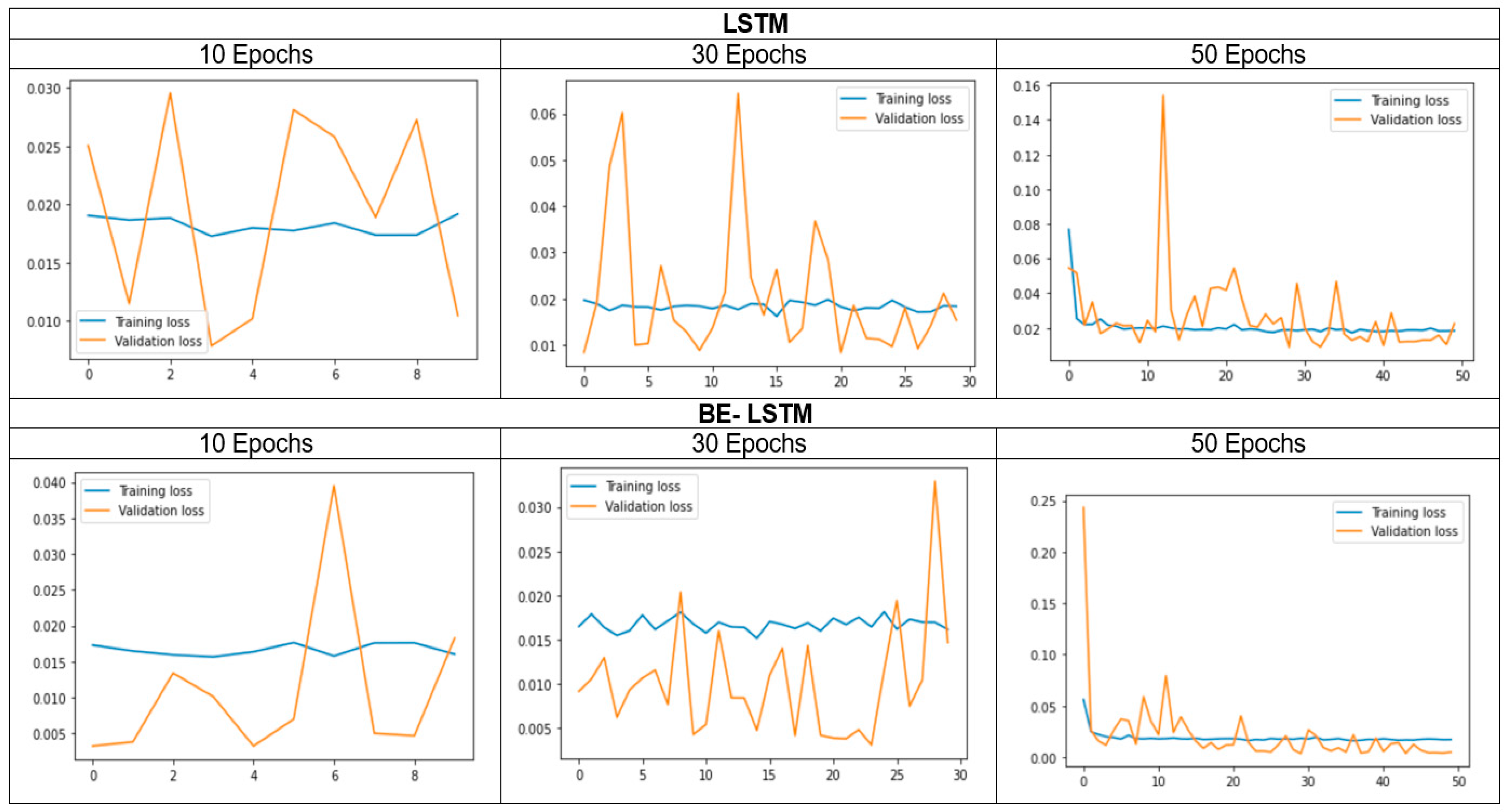
| Models | Epochs | Training Error | Validation Error | MSE | RMSE | MAPE |
|---|---|---|---|---|---|---|
| LSTM | 10 | 0.0192 | 0.0229 | 2,493,098 | 1578.95 | 10.66 |
| 30 | 0.01 | 0.0095 | 1,826,370 | 1351.43 | 9.05 | |
| 50 | 0.0167 | 0.0178 | 1,232,070 | 1109.98 | 6.62 | |
| Backward Elimination with LSTM | 10 | 0.0180 | 0.0171 | 465,470 | 682.25 | 5.33 |
| 30 | 0.0154 | 0.0165 | 393,554 | 627 | 4.55 | |
| 50 | 0.0148 | 0.0157 | 383,597 | 619.35 | 3.54 |
| Related Works | Models | Accuracy | Precision | Recall |
|---|---|---|---|---|
| (Ariyo et al. 2014) | ARIMA | 0.90 | 0.91 | 0.92 |
| (Khaidem et al. 2016) | Random Forest | 0.83 | 0.82 | 0.81 |
| (Asghar et al. 2019) | Multiple Regression | 0.94 | 0.95 | 0.93 |
| (Shen and Shafiq 2020) | Feature Expansion + Feature Selection + Principal Component Analysis + Long Short-Term Memory (FE+ RFE+PCA+LSTM) | 0.93 | 0.96 | 0.96 |
| Proposed method | LSTM | 0.84 | 0.83 | 0.84 |
| Backward Elimination with LSTM | 0.95 | 0.97 | 0.96 |
Disclaimer/Publisher’s Note: The statements, opinions and data contained in all publications are solely those of the individual author(s) and contributor(s) and not of MDPI and/or the editor(s). MDPI and/or the editor(s) disclaim responsibility for any injury to people or property resulting from any ideas, methods, instructions or products referred to in the content. |
© 2023 by the authors. Licensee MDPI, Basel, Switzerland. This article is an open access article distributed under the terms and conditions of the Creative Commons Attribution (CC BY) license (https://creativecommons.org/licenses/by/4.0/).
Share and Cite
Jafar, S.H.; Akhtar, S.; El-Chaarani, H.; Khan, P.A.; Binsaddig, R. Forecasting of NIFTY 50 Index Price by Using Backward Elimination with an LSTM Model. J. Risk Financial Manag. 2023, 16, 423. https://doi.org/10.3390/jrfm16100423
Jafar SH, Akhtar S, El-Chaarani H, Khan PA, Binsaddig R. Forecasting of NIFTY 50 Index Price by Using Backward Elimination with an LSTM Model. Journal of Risk and Financial Management. 2023; 16(10):423. https://doi.org/10.3390/jrfm16100423
Chicago/Turabian StyleJafar, Syed Hasan, Shakeb Akhtar, Hani El-Chaarani, Parvez Alam Khan, and Ruaa Binsaddig. 2023. "Forecasting of NIFTY 50 Index Price by Using Backward Elimination with an LSTM Model" Journal of Risk and Financial Management 16, no. 10: 423. https://doi.org/10.3390/jrfm16100423