Article

Global Spillovers of a Chinese Growth Slowdown

1
Board of Governors of the Federal Reserve System, Washington, DC 20551, USA
2
Bloomberg LP, New York, NY 10022, USA
*
Author to whom correspondence should be addressed.
J. Risk Financial Manag. 2022, 15(12), 596; https://doi.org/10.3390/jrfm15120596
Submission received: 2 September 2022 / Revised: 16 November 2022 / Accepted: 22 November 2022 / Published: 12 December 2022
(This article belongs to the Special Issue Central Banking and Financial Stability)

Abstract

:
This paper analyzes the potential spillovers of a slowdown in Chinese growth to the United States and the rest of the world. Through a combination of structural VAR and DSGE analyses, we find that (1) spillovers from China to the rest of the world have grown significantly in the past decade; (2) the negative growth spillovers to the United States are more modest than to emerging market economies—particularly for commodity exporters—or other advanced economies, primarily because the latter group has larger direct exposure in trade to China; and (3) although the United States has limited direct financial exposure to China, the negative spillovers to the U.S. economy are amplified significantly if the negative Chinese growth shock leads to adverse global risk sentiment and monetary policy in the United States is constrained in its reaction.
JEL Classification:
F30; G28; E60

1. Introduction

In the two decades since its accession to the World Trade Organization (WTO) in 2001, China has more than quadrupled its gross domestic product (GDP) per capita and played an increasingly central role in world commodities markets, international trade, and financial markets. While this remarkable rise has generated widespread benefits, observers are increasingly concerned about the potentially significant global spillovers from an abrupt slowdown in the Chinese economy. The reasonings behind these concerns vary: some observe that China’s financial system has seen a buildup of financial vulnerabilities after years of the government’s reliance on credit-fueled economic policies (European Central Bank 2017); others argue that an abrupt growth deceleration has frequently occurred in other economies reaching a similar stage of development as China’s (Pritchett and Summers 2014; Gauvin and Rebillard 2018). Furthermore, the early part of the COVID pandemic shows that a sudden disruption in the Chinese economy could lead to immediate and cascading effects on global markets.
Our paper adds to the body of literature by asking two questions: first, whether China’s connections with the rest of the world are large enough to generate economically important spillovers; second, whether financial or real transmission channels are more significant in generating those spillovers. Using a mixture of econometric and dynamic stochastic general equilibrium (DSGE) modeling work, we estimate the spillover effects of a sharp reduction in China’s GDP growth (“hard landing”) on the rest of the world, highlighting the transmission channel through global financial sentiment. We adopt a two-stage structural vector autoregression (SVAR) framework. In the first stage, we identify exogenous and domestically originated shocks to the Chinese GDP, accounting for how global variables affect China. In the second stage, we use auxiliary regressions to estimate the response to these shocks of a large set of outcome variables, which go beyond the variables included in the first-stage model and include GDPs in various countries or regions and global asset price variables. To shed light on the contribution of the sentiment channel, we compare and enrich the SVAR results with those from simulations of a large-scale DSGE, which takes into account volatilities in global asset price movements induced by China, calibrated from an event study from the 2015–2016 “China scare” episode.1
Our main findings can be summarized as follows. First, the SVAR estimates imply that an unexpected drop in China’s GDP growth would have sizable effects on global variables in the expected direction. In particular, the dollar would appreciate, U.S. long-term yields would fall, global Emerging Markets Bond Index (EMBI) spreads would rise, and world trade would fall (consistent with significant increases in emerging market economy (EME) risk premiums and safe-haven flows to the United States as well as China’s importance in global trade flows). In addition, there would be a substantial fall in global oil and metals prices, consistent with China being a major source of global demand for commodities.
Second, our second-stage auxiliary regressions suggest that the relative drops of economic activity in countries or regions around the globe are consistent with those found in the literature (Dieppe et al. 2018; Gauvin and Rebillard 2018), with a larger hit to those with higher trade exposure to China. More specifically, we find that the output loss in EME commodity exporters would be about three-fourths as large as the hit to China itself, about half as large for other EMEs, slightly more than one-third for advanced economies excluding the United States, and a more modest but not trivial effect in the United States.
Our DSGE model simulations suggest that volatility in global asset prices associated with an adverse Chinese growth shock could magnify the spillovers to advanced economies compared with that found in a standard DSGE model with the typical trade and endogenous financial channels. Furthermore, effective lower bound (ELB) constraints in the monetary policies of advanced economies can also amplify the spillovers. We find that in such an event, output losses in the United States could triple from a modest amount to about one-third of the hit to the Chinese GDP.
Our paper contributes to the literature by expanding on the existing methodologies to study spillovers from China and by testing for the importance of additional channels of transmission between China and the rest of the world. Many studies use vector autoregressive (VAR) models, but a well-known limitation of that approach is that researchers are often constrained to include only a limited set of variables in order to conserve degrees of freedom (Bernanke et al. 2005). Our two-stage approach allows us to include as many outcome variables as desired in the auxiliary regressions of the second stage, provided the first-stage VAR adequately identifies the exogenous Chinese output shock. More specifically, past studies have placed a stronger focus on the trade and commodity price channels; thus, the VARs used in those studies tend to include real variables (i.e., GDP and/or trade) and a few financial variables such as an oil or commodity price index and exchange rates. Because impulse responses could only be traced for the included variables, these studies were not able to produce the effects on other important financial outcome variables such as U.S. Treasury bond yields, global EMBI spreads, and equity indices. A similar critique applies to the global vector autoregressive (GVAR) models.2 While GVARs can account for the correlations between all the variables and the countries included, the methodology limits the number of variables per country or economic bloc that can be studied. An alternative approach that relaxes these constraints is the factor-augmented VAR (FAVAR), which allows information from a very large number of variables to be collapsed into a few factors. We do not use this methodology because the interpretation of the factors in the model is often unclear and, in turn, would make it difficult to interpret the structural shocks.
Another contribution of our paper is that it highlights the role of global risk sentiment as an important transmission channel of an unanticipated slowdown in Chinese growth to countries that do not have large direct trade and financial exposure to China, such as the United States. We also highlight the amplifying effects of the zero-interest lower bound in advanced economies for the transmission of shocks emanating from China. Our results are similar to Gilhooly et al. (2018) and Dieppe et al. (2018), who also found that the spillovers are larger when conventional monetary policy is constrained by the ELB. Those papers use similar empirical methodologies to estimate the global spillovers from a slowdown in China, obtaining results quite consistent with ours. However, our paper is relatively more focused on economic and, especially, financial spillovers to the United States.
The remainder of the paper is organized as follows. Section 2 provides a literature review. Section 3 discusses some stylized facts about China’s financial vulnerabilities and the evolution of China’s economic and financial linkages (both direct and indirect) with the rest of the world. Section 4 presents results from the two-stage SVAR analysis. Section 5 compares the results from the SVAR with that of our DSGE model to illustrate the role that global asset price volatility and the ELB could play in enhancing spillovers from a China growth shock. Section 6 concludes.

2. Literature Review

The sustainability of China’s rapid GDP growth rates is being addressed in a growing body of literature. Some academic papers have argued that China’s current level of development has entered a stage where the idea of “economic convergence” (whereby economies start to slow as they develop further) would necessarily entail a deceleration of growth (Lee and Hong 2010; Eichengreen et al. 2012; Barro 2016).3 Other researchers have concluded from the global historical growth experience that periods of rapid growth rarely persist, implying a high statistical likelihood of an abrupt growth slowdown in China in the coming years (Pritchett and Summers 2014). Other papers have shown that economies that went through a sustained period of investment-driven growth tend to experience sharp growth decelerations in their transition to consumption-driven growth (Gauvin and Rebillard 2018).
Observers have also raised concerns that vulnerabilities have built up in China’s financial system, increasing the likelihood of a Chinese financial crisis. In particular, nontraditional financial intermediation activities involving opaque products have proliferated, traditional banks have deepened their connections to shadow-banking activities, and property price valuations across major Chinese cities have remained elevated for several years (Hsieh and Klenow 2009; Song et al. 2011; Manu et al. 2018; Li et al. 2014; Perry and Weltewitz 2015; Li 2016; Ehlers et al. 2018). Factors that have been shown to be predictive of financial crises in the literature about early warning indicators have been flashing red for China. For example, Aldasoro et al. (2018) point out that China’s credit-to-GDP gap and debt service ratios have exceeded the thresholds that tend to predict at least two-thirds of banking crises occurring within three years in a sample of advanced and emerging economies. China’s corporate debt-to-GDP ratio has also exceeded the 90 percent threshold that Cecchetti et al. (2011) identified as the point when debt becomes a drag on growth. Several studies also share similar findings (Reinhart and Rogoff 2011; Laeven and Valencia 2013; Chen and Kang 2018; Dell’Ariccia et al. 2016; Lee et al. 2020).
Those heightened concerns have led to a growing body of literature that quantifies the economic spillovers to the rest of the world in the event of an abrupt growth deceleration in China. A consensus finding in recent studies is that spillovers from China to commodity-exporting countries and emerging Asian economies outside of China are significant and large through the commodity price and trade channel. Dieppe et al. (2018), for example, find that the output loss for oil exporters is nearly half as large as the shock to China itself, while Gauvin and Rebillard (2018) find similar-sized spillovers to emerging Asian commodity-exporting countries as well as those in Latin America (see also Erten 2012; Ahmed 2017; Ma et al. 2017). By comparison, we find even larger spillovers, with the output loss for EME commodity exporters around three-fourths as large as the shock to China. While likely smaller, the exact magnitude of spillovers from China to advanced economies, in particular to the United States, is more uncertain and debated. Many studies have found U.S. GDP growth to be insignificantly affected by a slowdown in China, though the spillovers are significant in the reverse direction (Pang and Siklos 2016; Huang et al. 2018). Fontaine et al. (2017) find that the spillovers from China are only significant to the United States during U.S. recession periods. Dieppe et al. (2018) find that a China hard landing similar to the one we simulate in this paper would lower U.S. GDP by 0.9 to 1.5 percent, which is similar to our estimate when we do not include additional financial spillovers. The explanation for limited spillovers to the advanced countries is that they tend to have limited direct trade or financial exposure to China. However, the large co-movements in global asset prices (McCauley and Shu 2019) in the aftermath of China’s surprise depreciation in 2015 highlighted that fears of a Chinese hard landing could trigger a global risk-off event. Such an event could indirectly transmit the slowdown to advanced economies through volatility in global asset prices, even with limited direct trade and financial exposures to China.
In this paper, we quantify the spillovers of a sharp slowdown in China to the rest of the world, highlighting the importance of the financial and sentiment channels. These channels are most important to the United States, given the relatively small direct exposure of U.S. financial institutions to China. As noted previously, we use both a two-stage VAR approach and a DSGE model to assess the magnitude of spillovers from China, which incorporate these financial and sentiment features.

3. Sources of Vulnerabilities in China and Transmission Channels to the Rest of the World

This section provides an overview of the most important financial vulnerabilities in China and the degree of connectedness between China, the United States, and the rest of the world.

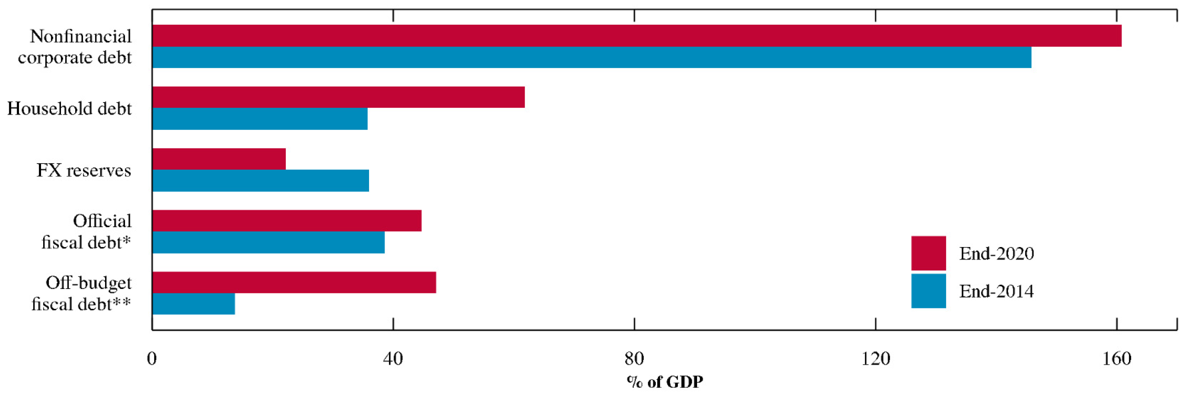
3.1. Financial Vulnerabilities

China has developed notable financial vulnerabilities since the global financial crisis (GFC). The financial system has grown rapidly and become very large in both absolute size and in relative terms for China’s level of economic development. This growth, by itself, does not necessarily signal vulnerabilities, but several developments in the Chinese financial system over the past several years are concerning. China’s nonfinancial private credit has more than doubled since the GFC to about 35 trillion dollars in 2020, almost the same as that for the United States and much larger than for some of the largest advanced economies. This level of debt also accounts for roughly 220 percent of GDP, a threshold that has often been followed by adverse consequences.4 Besides businesses being highly leveraged, household indebtedness has also increased materially in the past few years. The banking system, which is by far the largest in the world in terms of total assets, reports adequate buffers, but banks are heavily exposed to risky corporate and local government debt. Additionally, the large nonbank financial sector could be susceptible to liquidity problems and runs. It bears noting, though, that the Chinese government also has substantial resources to support any troubled financial and nonfinancial institutions.
Turning to an assessment of individual sectors, some vulnerabilities in the financial sector have increased since just before 2015–2016, when Chinese financial markets were shaken by the discrete devaluation of the renminbi, capital outflows, and the subsequent large movements in Chinese equity prices. Although large banks’ capital levels appear adequate, they may prove insufficient in the event of a pronounced slowdown in economic activity and rising delinquencies, especially when taking into account the banks’ deep connections to shadow-banking activities and institutions. The Chinese shadow-banking sector is focused on credit intermediation through nontraditional products, such as wealth management products (WMPs).5 These products compete with bank deposits for corporate and household savings, typically offering closed-ended instruments with short maturities. The proceeds of this funding are invested in longer-term assets such as corporate loans or bonds. The opaqueness of these products and the expectation that guaranteeing banks or the government will bail them out in periods of stress may lead investors to underestimate their risks. Aware of these risks, Chinese regulators have focused on curtailing the growth of the riskiest activities since 2017 with some success.
The nonfinancial corporate sector may also have sizable vulnerabilities. The corporate debt-to-GDP ratio increased by about 20 percentage points between the end of 2014 and 2020, standing at over 160 percent at end-2020 (Figure 1). Similarly, household debt has risen briskly due to the sharp increase in mortgage borrowing that has accompanied the rapid rise in house prices, especially in the largest cities. The household debt-to-GDP ratio has jumped 15 percentage points from 2014 to 2020 and has reached a level (more than 50 percent of GDP) that is high for an EME.
Balancing these vulnerabilities are strong positions in the external and sovereign sectors. China has more than $3 trillion in foreign exchange reserves and a current account surplus. Reserves are now below the highs of 2014–2015, but they remain high.
The ultimate backstop for a financial stability event is intervention by the sovereign. In China, such intervention is easier because the government has significant resources, and the financial system is closed—with little dependence on borrowing from abroad—and largely state-controlled. However, China’s fiscal space has decreased in the past five years. To be sure, it still has a relatively low ratio of official fiscal debt of close to 45 percent of GDP, which is just slightly higher than it was in 2014 (Figure 1). However, this debt stock does not include off-budget fiscal items such as the liabilities of local government financing vehicles (LGFVs).6 After adding these off-balance-sheet items, the augmented sovereign debt level is an estimated 92 percent of GDP, which is on the very high end for other EMEs.
The sizable vulnerabilities in the Chinese financial system could be fertile ground for an event that threatens financial stability.7 We do not take a stand with regard to the exact triggers for such an event, but some potential examples of triggers include a series of local government and corporate bond defaults that dent consumer and investor confidence, a large property sector bust hurting consumer investment and spending, and a renewed escalation of trade tensions hurting corporate profits and spending. Any of these triggers could precipitate sharp and stressful slowdowns in the economy.

3.2. China’s Trade and Financial Linkages with the Rest of the World

China’s global importance has grown rapidly over the past two decades. To quantify the evolution of the relative importance of China across many dimensions, we construct a time series of country rankings based on financial and macroeconomic indicators.8 The ranking is composed of indicators grouped into three categories: size, interconnectedness, and U.S. interconnectedness. The first component measures the size of a country on various metrics. The second component measures the overall linkages of a country to other economies. The third component focuses more specifically on a country’s linkages with the United States. Our motivation for distinguishing between the second and third components is that it helps to identify to what extent the United States may be directly exposed to China versus how it might be indirectly affected by China through China’s links to other countries that are closely linked to the United States.
The methodology to rank countries follows a multistep approach. First, countries are ranked based on each individual data series for every year. Second, rankings are averaged across these series within each category (and year), and countries are ranked again based on these averages. Last, the average ranking across the three categories is calculated, and this average is used to construct the overall ranking.9
Figure 2 presents the index for China between 2000 and 2020. China, in the early 2000s, ranked as high as 16th (using the overall ranking) among our sample of 176 countries, but by 2020 it ranked fifth. The largest gains were in size and overall interconnectedness. Although China has become more connected with the United States, it still lags compared to the linkages that United States has with other advanced economies. This property suggests that indirect linkages of China with the United States through other countries may be quite important. The evidence thus highlights not just the growing importance of China in the global financial system, but also how the stronger ties between China and the rest of the world could amplify the transmission of shocks originating in China to the United States.

3.3. U.S. Financial Institutions’ Direct and Indirect Exposures to China

The international banking literature has noted that shocks can be propagated through the activities of global financial institutions (Buch and Goldberg 2015; Cetorelli and Goldberg 2012; Correa et al. 2021). To assess the importance of this transmission channel, through both direct and indirect exposures of the U.S. financial sector to China, we use information on consolidated banking exposures from the BIS consolidated banking statistics.10
As shown in Table 1, direct exposures of U.S. financial institutions to Chinese residents seem rather modest, with the consolidated U.S. bank claims on Chinese and Hong Kong residents totaling $228 billion, or 16 percent of the reporting banks’ Tier 1 capital, at end-June 2021.
However, spillovers to U.S. financial institutions could also occur through at least four types of exposures that indirectly transmit stress in China to their balance sheets: (1) exposure of other financial systems to China, such as banks in the United Kingdom and Singapore11 (Table 2 and Table 3); (2) exposure to holdings of Chinese financial assets12; (3) exposure to commodity exporters, which are highly exposed to China13 (Table 4); and (4) exposure to activities of Chinese banks in U.S. short-term funding markets14 (Figure 3 and Figure 4; Table 5). Individually, each of these exposures represents a modest fraction of U.S. banks’ Tier 1 capital or of other financial institutions’ assets. However, jointly, these exposures, combined with the direct exposure to China, could affect a non-negligible portion of the portfolios of U.S. banks and nonbanks.

4. Quantifying the Spillovers

In this section, we estimate the effect of a Chinese growth slowdown on a large set of global and country-specific macroeconomic and financial variables. The number of impact variables we are interested in poses a methodological challenge because most empirical methodologies can only handle a limited number of variables simultaneously. We overcome this challenge by using a two-stage approach—specifically a two-stage SVAR—that allows us to estimate the effect of a China’s GDP growth slowdown caused by domestic factors on a large number of macroeconomic and financial variables.

4.1. Methodology

4.1.1. First Stage

In the first stage, we use an SVAR model to decompose unexpected fluctuations in Chinese GDP growth into foreign and domestically originated shocks and then analyze the effects of exogenous domestic shocks to Chinese economic growth on a set of global variables. U.S. monetary policy shocks, autonomous changes in global risk sentiment, commodity price changes originating in the rest of the world, and foreign fiscal policy shocks are examples of foreign shocks to China’s GDP. Exogenous changes in China’s aggregate productivity or in credit conditions are examples of domestic shocks to China’s GDP.
Specifically, we estimate a nine-variable VAR model using quarterly data from 2002:Q1 to 2017:Q4.15,16 Of these nine variables, eight represent global financial and macroeconomic conditions—U.S. long-term yields, broad nominal dollar, VIX, EMBI spreads, oil prices, metals prices, GDP growth for the G-7 economies, and growth of global imports excluding Asian EMEs—and the remaining variable is Chinese GDP growth. In order to have greater confidence that we have identified exogenous domestically originated shocks to the Chinese GDP, we assume that Chinese GDP growth is affected contemporaneously (within the quarter) by all other variables, but that Chinese GDP growth can affect the other variables only with a lag.17 That is, Chinese GDP growth comes last in a recursive contemporaneous causal ordering. Any change in China’s GDP growth that cannot be accounted for by developments (including contemporaneously) in these global indicators is taken to originate from domestic factors. After identifying exogenous Chinese GDP shocks, the effects of these shocks on the global variables included in the model are traced out.
While this approach is not criticism-free, we view it as balanced because it provides a split between foreign- and domestic-originated shocks to China’s GDP that sits between two possible sources of misspecification. Using this approach, we could be overestimating the domestic-originated GDP shocks if we had omitted some external factor of great importance for China’s economy that was largely uncorrelated with the other eight variables in the model. We could also be underestimating the domestic-originated GDP shocks if China’s GDP was a very important driver of the variation in the other eight variables in the model, and, therefore, our estimates of externally generated shocks to China’s GDP were simply the effect of China’s GDP on those external variables.

4.1.2. Second Stage

In the second stage, we estimate separate bivariate SVAR models, with one variable always being the identified domestic shock to China’s GDP growth from the first-stage model and the second variable being different outcome variables. These second outcome variables include other global variables of interest that are not included in the first-stage model or country-specific variables (most notably GDP growth of different countries). The second-stage models are then used to trace out the effects of a Chinese GDP growth shock on these other outcome variables of interest. Because we have already identified exogenous Chinese GDP growth shocks from the first stage, we feel comfortable putting them first in the causal ordering in the second-stage SVARs. Moreover, by using the domestic China GDP shocks that were identified in the first stage, according to Plagborg-Møller and Wolf (2021), the estimates from the second stage are akin to using an instrument to structurally estimate the effects of the domestic China GDP shock on the other variable included in the bivariate VAR. The results of Plagborg-Møller and Wolf (2021) provide a strong backing to the second-stage estimation, because these authors showed that structural estimation with an instrument can be carried out by putting the instrument first in a recursive VAR, and this approach can even be performed under the noninvertibility of the model. This result is directly applicable to the second-stage estimations because we use a recursive identification scheme with the domestic China GDP shock ordered first.

4.2. Results

First, note that, in both stages, the estimated models include a constant term, a linear trend, and a dummy variable for the years 2008 and 2009 to account for the GFC. We include the linear trend to account for possible trends in the data (e.g., China’s GDP growth rate has been on a downward trend), and we include the GFC dummy variable because we see the GFC as an extreme event and do not want the analysis to be overly influenced by the unusual interactions of the variables during this period.18

4.2.1. First-Stage Results

Figure 5 shows the response of all the variables included in the VAR model to a negative unit domestic China GDP shock (equivalent to a 1 percentage point decrease in quarter-on-quarter Chinese GDP growth).19 Starting with the financial variables, our results show that, in response to a surprise decrease in China’s GDP, U.S. long-term yields decrease, the dollar appreciates, and the VIX and EMBI spreads both increase, as would be expected. These results are consistent with a negative China GDP surprise leading to a retrenchment of global risk appetite. This situation leads to safe-haven capital flows from risky to safe assets that push U.S. yields lower. Our results also show that both oil and metals prices decrease substantially following the adverse China output shock, a result that is also not surprising given the importance of China for global demand for commodities. We also find that a negative China GDP surprise pushes both aggregate G-7 GDP growth and world trade excluding EME Asia lower.
How much of the fluctuation in global variables and in China’s own GDP growth can be explained by domestic Chinese growth shocks? To address this question, we compute the forecast error variance decompositions (FEVDs) of the variables in the VAR model. The results, presented in Table 6, show that, overall, fluctuations in China’s GDP growth account for a significant proportion of fluctuations in several of the global variables included in the model. Of the variables included in the first-stage VAR, fluctuations in China’s GDP growth are most important for fluctuations in the dollar and the EMBI spreads as well as for commodity prices and world trade.
For the decomposition of China’s own GDP growth, it is interesting that about one-fifth (over the short run) to half (over the longer run) of the fluctuations are accounted for by external shocks. This observation is consistent with China being a conduit of global demand because of its importance in global supply chains. In addition, the fact that the domestic component of the GDP shock accounts for close to 80 percent of the overall unexpected fluctuations in China’s GDP suggests that our identification assumptions are very unlikely to be causing the domestic component of China’s GDP shocks to be significantly underestimated. It also suggests that the China GDP shocks we identify are not all that different from what we would have obtained had we put China’s GDP first in the VAR instead of last, as we did.

4.2.2. Second-Stage Results

The second-stage results, presented in Figure 6, focus on the effects of Chinese growth on growth elsewhere in the world.20 A negative Chinese GDP shock substantially brings down growth of EMEs elsewhere, especially those of commodity exporters. Growth in advanced economies other than the United States, which we label advanced foreign economies (AFEs), is also affected significantly, while the effect on U.S. growth, although still negative, is more modest.
Similarly to what is done in the first stage, we also compute the FEVDs for the second-stage outcome variables. The results are presented in Table 7. As can be seen from this table, China’s GDP growth shocks account for a significant proportion of growth fluctuations in other EMEs (especially commodity exporters)—akin to China’s share of global GDP—but less so for advanced economies. Compared with other advanced countries, the United States is also much less exposed to China shocks.
The results in Figure 6 and Table 7 are consistent with growth in EMEs being highly connected to China’s economic growth, especially through commodity trade linkages. AFEs are, on average, also more open than the United States and therefore more exposed than the United States to shocks from China affecting global trade.

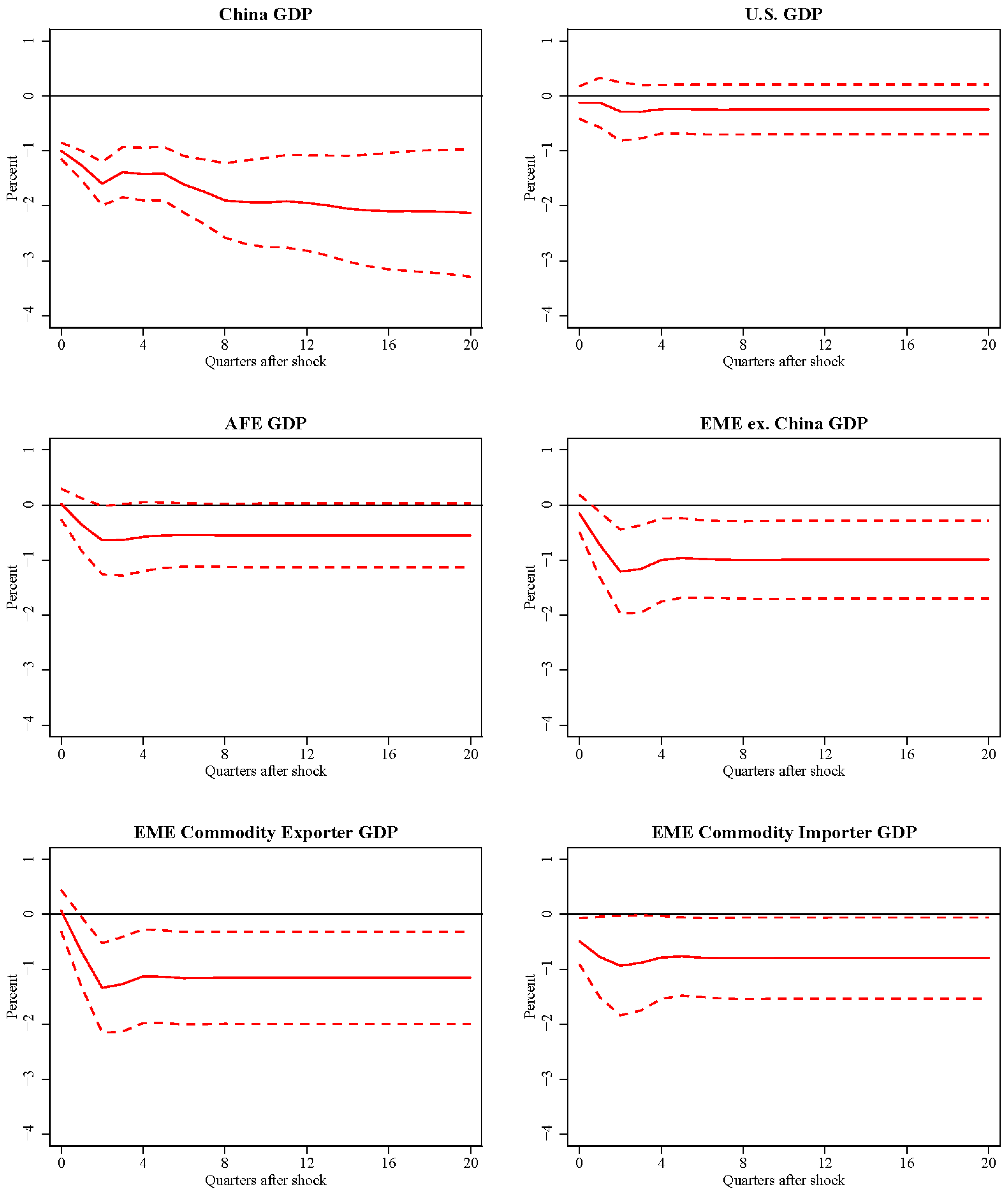
4.2.3. Spillovers of a China GDP Growth Slowdown

To analyze the global spillovers from a financial distress scenario in China, we first need to identify concretely the impact of the distress scenario on China’s own GDP growth. Specifically, we consider two different hypothetical scenarios with varying levels of distress that are calibrated to different points of the historical distribution of growth slowdowns following financial distress. In the “adverse” financial distress scenario, we assume a 4 percent decline in output relative to baseline, which corresponds to the 50th percentile of growth slowdowns in the distribution of historical financial crises.21 Yet in the “severely adverse” financial distress scenario, we assume an 8½ percent decline in output relative to baseline, which corresponds to the 80th percentile of historical growth slowdowns during financial crises.
We use these two scenarios to quantify the potential effects of extreme events in China on the global economy based on the SVAR models described before. Specifically, to estimate the spillover effects of the two adverse scenarios for China’s GDP, we simulate a sequence of shocks to China’s GDP growth rate that generates a response from China’s GDP equal to that assumed in each scenario, as shown in the top left panel of Figure 7.22 We then feed the two sequences of shocks (one for each scenario) into the estimated SVAR models to obtain an estimate of the response of the variables of interest to these shocks. Figure 7 also shows the response of GDP for various regions and countries, and Figure 8 shows the response of several financial variables.
The results in Figure 7 show that the hit to economic activity around the world can be quite substantial. The effects on U.S. GDP are relatively modest, while those on AFE GDP are more than twice as large as that on the United States. In the severe scenario and relative to baseline, U.S. output declines slightly more than 1¼ percent, and AFEs’ output declines more than 3¼ percent (just over one-third of the hit to Chinese GDP itself). The GDP in other EMEs falls close to 6 percent below baseline, over two-thirds of the decline in Chinese GDP. Among EMEs, commodity exporters are hit much harder than commodity importers.
Regarding the effects on financial variables (Figure 8), U.S. long-term yields fall substantially, which suggests that the negative effects on yields of increased flows into safe-haven assets dominate the positive effects of any Chinese selloff of reserves. Global EMBI spreads rise, with a peak increase of over 350 basis points in the severe scenario, and risk aversion (as measured by the VIX) increases substantially. The broad nominal dollar appreciates (about 7 percent and 15 percent in the mild and severe scenarios over roughly two years, respectively). Finally, with China being a key driver of world commodity demand, oil and metals prices tumble in both scenarios.

5. Spillovers Using DSGE Model Simulations
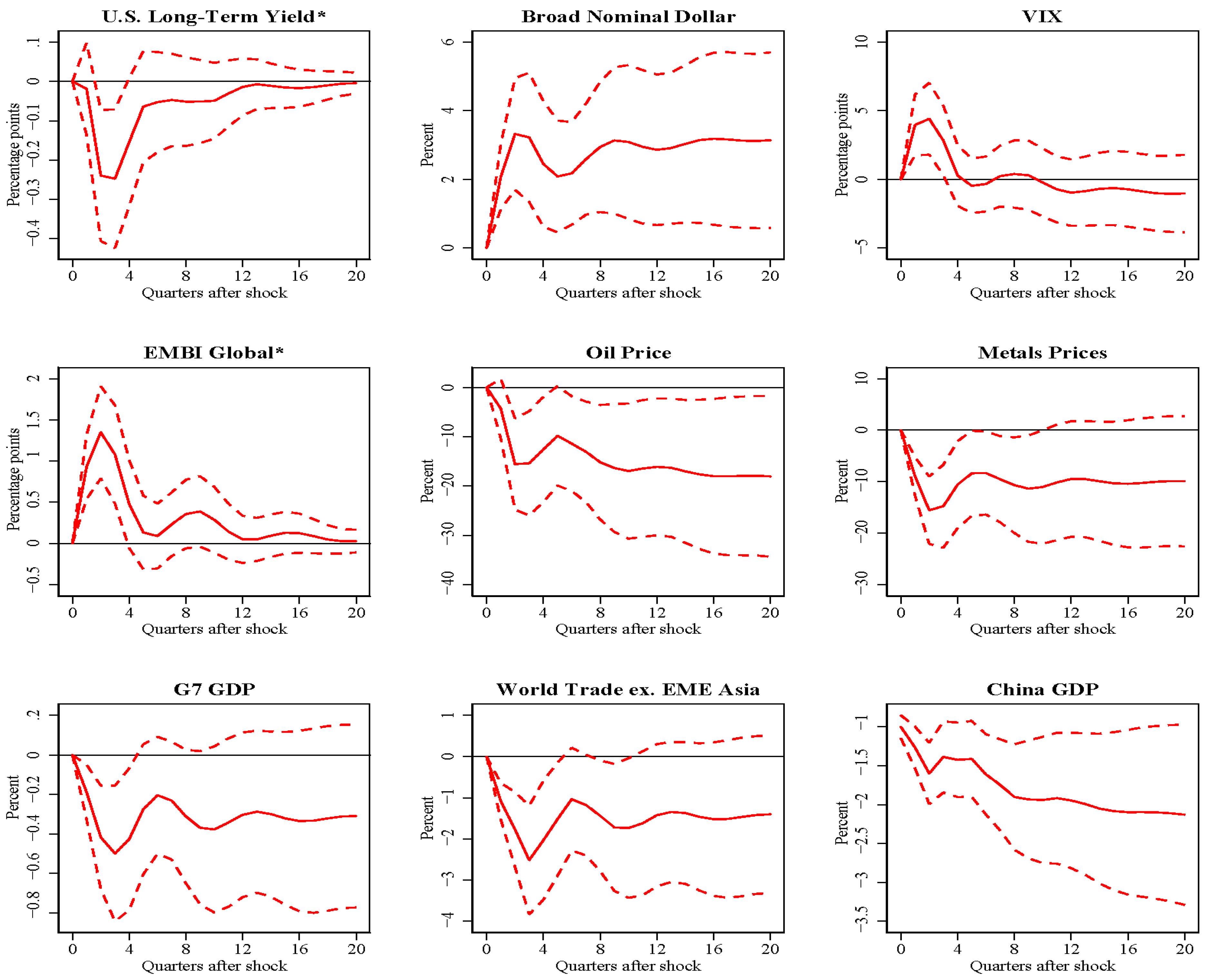
In this section, we highlight the amplifying roles played by the global financial spillovers and zero-lower-bound constraints in the AFEs. These financial spillovers were not very prominent over much of our sample period in the SVAR analysis, but our motivation for including them is that they were evident in the response of global financial markets to the 2015–2016 China scare episode in which adverse financial developments in China triggered outsized movements in global financial markets.
To quantify the role of these channels, we use the Federal Reserve Board’s open economy SIGMA model. It is a DSGE model that incorporates standard real and financial transmission channels but also adds extra financial transmission to quantify how much these additional financial channels can amplify the real spillovers to foreign GDP compared with the traditional DSGE model, which only includes the trade channel and standard endogenous financial responses. We simulate the extra global asset price movements associated with a China growth shock by calibrating them to those observed in the most recent hard-landing scare in China in 2015–2016 (labeled the China scare).23
The 2015–2016 China scare episode highlights that, despite the limited direct trade and financial linkages of the United States with China, adverse scenarios in China could roil global financial markets significantly. Sustained depreciation of the Chinese currency and capital outflows from China during this episode had unusual reverberations for global markets, with significant declines in equities around the world, a retrenchment of global risk appetite, an increase in U.S. and emerging market corporate bond spreads, and a fall in long-term advanced-economy yields. To the extent that problems in China could lead to a hit to the U.S. economy and financial system, they would likely come indirectly through any disruptions to global (including U.S.) financial markets that a China distress scenario may engender. We calibrated the extra financial spillover shocks in the DSGE models from three narrow event windows during the 2015–2016 China scare episode24:
(1)
A sudden, discrete 2 percent devaluation of the Chinese renminbi against the dollar occurred on 11 August 2015, which triggered a depreciation in many emerging market currencies and appreciation of the U.S. dollar.
(2)
A precipitous drop in the Chinese stock market occurred on 24 August 2015, that became known as “China’s Black Monday”, where the Shanghai stock index declined by almost 8½ percent of its value overnight.
(3)
Two large and sudden declines in the Chinese stock market of more than 7 percent occurred between 4–7 January 2016, that led to the trigger of automatic circuit breakers that halted trading.25 Capital outflows continued during these episodes.
Table 8 reports the changes and percent returns for select global financial assets and indicators before and after the Chinese events previously described. We find that during these events the broad dollar index appreciated by about ¾ percent, with larger appreciations against EME currencies than AFE currencies. In addition, world equity markets fell between 3 and 4½ percent, and investor risk appetite as measured by the VIX and VDAX decreased. Along with the significant declines in global equities and a retrenchment of global risk appetite, we find that flight-to-safety flows lowered long-term AFE yields, as negative market shocks from China spilled over to assets abroad.
To put the above numbers into perspective, the spillovers from the China market turbulence roughly correspond to the 1 percent tail of the distribution for each financial asset, computed from the overall historical experience discussed in the previous subsection.
We begin the DSGE analysis by first simulating the spillover effects from a negative unit Chinese growth shock on real GDP to the rest of the world in the standard SIGMA model, which has built-in standard trade channels and a small endogenous response of financial variables.26 Then, we construct extra financial shocks using the magnitudes suggested by the event windows provided in Table 8, mapping them into the extra financial shocks in the exchange rate risk premium, household confidence, and corporate spreads in U.S. and AFE blocs in the SIGMA model.27
Panels C and D of Figure 9 show the effects of AFE and U.S. GDP under both assumptions. Starting in the scenario without the additional financial effects, in the Chinese “medium adverse” scenario, U.S. real GDP (panel D) would fall by a maximum of about ¾ percent below baseline and in the “severely adverse” scenario by about 1 percent. The U.S. responses without financial spillovers are significant but not large.28 AFE output falls by about ¼ percentage point more than that of the United States in the two scenarios with standard spillovers.
The adverse effects on advanced economies from an adverse growth shock originating in China are notably bigger if turmoil in China causes reverberations in other financial markets similar to those implied by the event study of the 2015–2016 episode we presented earlier. The solid lines of panels C and D depict these circumstances for both the medium and hard-landing scenarios in China. U.S. GDP falls a little more than 1 percent in the medium scenario (similar to the VAR results estimated on the post-WTO accession sample) and just shy of 3 percent in the hard-landing scenario; these effects are about one-third of the hit to the Chinese economy. In the AFEs, output falls by about 1½ percentage points and 3¾ percentage points in the two scenarios, respectively.
According to these results, the spillovers to advanced economies as a whole from a China crisis and associated problems in other EMEs would be significantly bigger than we have observed in previous EME crises because of the global risk sentiment channel. Another important reason for stronger spillovers could be the limited scope for monetary policy to respond appropriately to negative shocks if several advanced economies are at the ELB. While in the simulations the U.S. policy rate starts sufficiently away from the ELB, we assume that the constraint on monetary policy in the AFEs becomes binding in the simulation for the hard-landing scenario with financial spillovers (this reflects generally lower policy rates in some AFEs).
In Figure 9, we show the response of AFE real GDP (panel E) and U.S. real GDP (panel F) under three assumptions. The red line represents the effect of the hard landing in the presence of the ELB.29 The green line shows the response of GDP if the ELB was not binding, but the calibrated shocks stayed the same. Finally, the black dashed line illustrates the effect on GDP if we rescaled the shocks to match the same targets as in the main simulation. There are two takeaways from the figure. First, the ELB, if not accompanied by QE, forward guidance, or fiscal policy changes, results in far worse outcomes for the advanced economies, as GDP falls by an additional 1 percentage point. Even fixing the size of the crisis in the emerging markets, GDP in the AFEs falls ¾ percentage point more. Second, while the ELB scenario might provide an upper bound on the effects of constrained policy (abstracting from debt-sustainability issues that might arise in some advanced economies), the rescaled simulation in the absence of the ELB might give us a good sense of the “best” case scenario in which unconventional policy effectively offsets the constraint, as some recent work has suggested was the case for the GFC. The most realistic scenario probably lies somewhere in between.

6. Conclusions

This paper documents the evolving macroeconomic and financial linkages between China and the rest of the world and assesses the impact of various adverse scenarios in China on the United States and the rest of the world using a combination of SVAR and DSGE models. We find that a hard landing in China would have consequential spillovers to the global economy, including the U.S. economy. In particular, there would be substantial hits to output in both EMEs and advanced economies. The United States would also experience some output losses under the adverse China growth scenarios posited in this paper, but less so than in EMEs and in other advanced economies due to the relatively smaller direct exposure to China. However, despite limited direct financial linkages between the United States and China, the spillovers of a China shock to the U.S. economy could be amplified if they impacted global financial markets through reduced global risk taking. The negative growth effects could be further magnified by zero-lower-bound constraints in the monetary policies of advanced economies. All in all, a Chinese hard landing would be a big global event and lead to serious negative spillovers to economic growth around the world, especially if it roiled global financial markets.

Supplementary Materials

The following supporting information can be downloaded at: https://www.mdpi.com/article/10.3390/jrfm15120596/s1.

Author Contributions

Conceptualization, S.A., R.C., D.A.D., N.G., J.H., A.J., E.L. and A.W.; methodology, S.A., R.C., D.A.D., N.G., J.H., A.J., E.L. and A.W.; software, S.A., R.C., D.A.D., N.G., J.H., A.J., E.L. and A.W.; validation, S.A., R.C., D.A.D., N.G., J.H., A.J., E.L. and A.W.; formal analysis, S.A., R.C., D.A.D., N.G., J.H., A.J., E.L. and A.W.; investigation, S.A., R.C., D.A.D., N.G., J.H., A.J., E.L. and A.W.; resources, S.A., R.C., D.A.D., N.G., J.H., A.J., E.L. and A.W.; data curation, S.A., R.C., D.A.D., N.G., J.H., A.J., E.L. and A.W.; writing—original draft preparation, S.A., R.C., D.A.D., N.G., J.H., A.J., E.L. and A.W.; writing—review and editing, S.A., R.C., D.A.D., N.G., J.H., A.J., E.L. and A.W.; visualization, S.A., R.C., D.A.D., N.G., J.H., A.J., E.L. and A.W.; supervision, S.A., R.C., D.A.D., N.G., J.H., A.J., E.L. and A.W.; project administration, S.A., R.C., D.A.D., N.G., J.H., A.J., E.L. and A.W.; funding acquisition, S.A., R.C., D.A.D., N.G., J.H., A.J., E.L. and A.W. All authors have read and agreed to the published version of the manuscript.

Funding

This research received no external funding.

Data Availability Statement

Data will be provided upon reasonable request.

Acknowledgments

We thank William Barcelona and Martin Sicilian for their excellent research assistance. We also thank Kun Mo, Steve Kamin, Beth Anne Wilson, and the participants at the China Expert Network workshop held at the Hong Kong Monetary Authority for their useful comments. The views expressed in this paper are solely the responsibility of the authors and should not be interpreted as reflecting the views of the Board of Governors of the Federal Reserve System, Bloomberg, or any other person associated with these institutions.

Conflicts of Interest

The authors declare no conflict of interest.

Notes

1
Using the DSGE model also allows us to provide a more forward-looking estimate in some regards, as the estimation of the SVAR necessarily forces us to use a long-time span in the data.
2
Ericsson et al. (2014) use both VAR and GVAR models to study the effects on global growth of a China GDP growth slowdown and find that the results based on the two models are broadly comparable (especially in the short-to-medium term).
3
Barro (2016) predicted China’s per capita growth rate in a conditional-convergence framework estimated from a large panel of countries. He estimated China’s per capita growth rate in 2015 to be 3.5 percent and declining, in contrast to the official 6 to 7 percent per year. He concluded that it is unlikely that China can deviate in the long run from the results predicted by global historical growth experience.
4
Almost half of the 11 countries that have sustained this level of debt as a percent of GDP experienced a financial crisis within five years of crossing this threshold.
5
The main products in the Chinese shadow-banking sector are trust company loans, entrusted loans, and WMPs. Trust companies manage assets for high-net individuals and institutions and invest in a range of products including bank loans and corporate bonds and loans. Entrusted loans are loans made by one nonfinancial firm to another nonfinancial firm, with a bank serving as an intermediary. WMPs are short-term investment products, often marketed by banks that invest in both equity and fixed-income products.
6
LGFVs are entities founded by local governments to finance projects on their behalf. They enjoy implicit debt repayment support but are legally separate from the government. The use of these off-budget vehicles has greatly expanded after the GFC. In recent years, the central government has attempted to clamp down on this off-budget borrowing by prohibiting local governments from providing support to LGFVs while at the same time allowing local governments greater leeway to borrow on-budget. Nonetheless, LGFV borrowing has continued to grow.
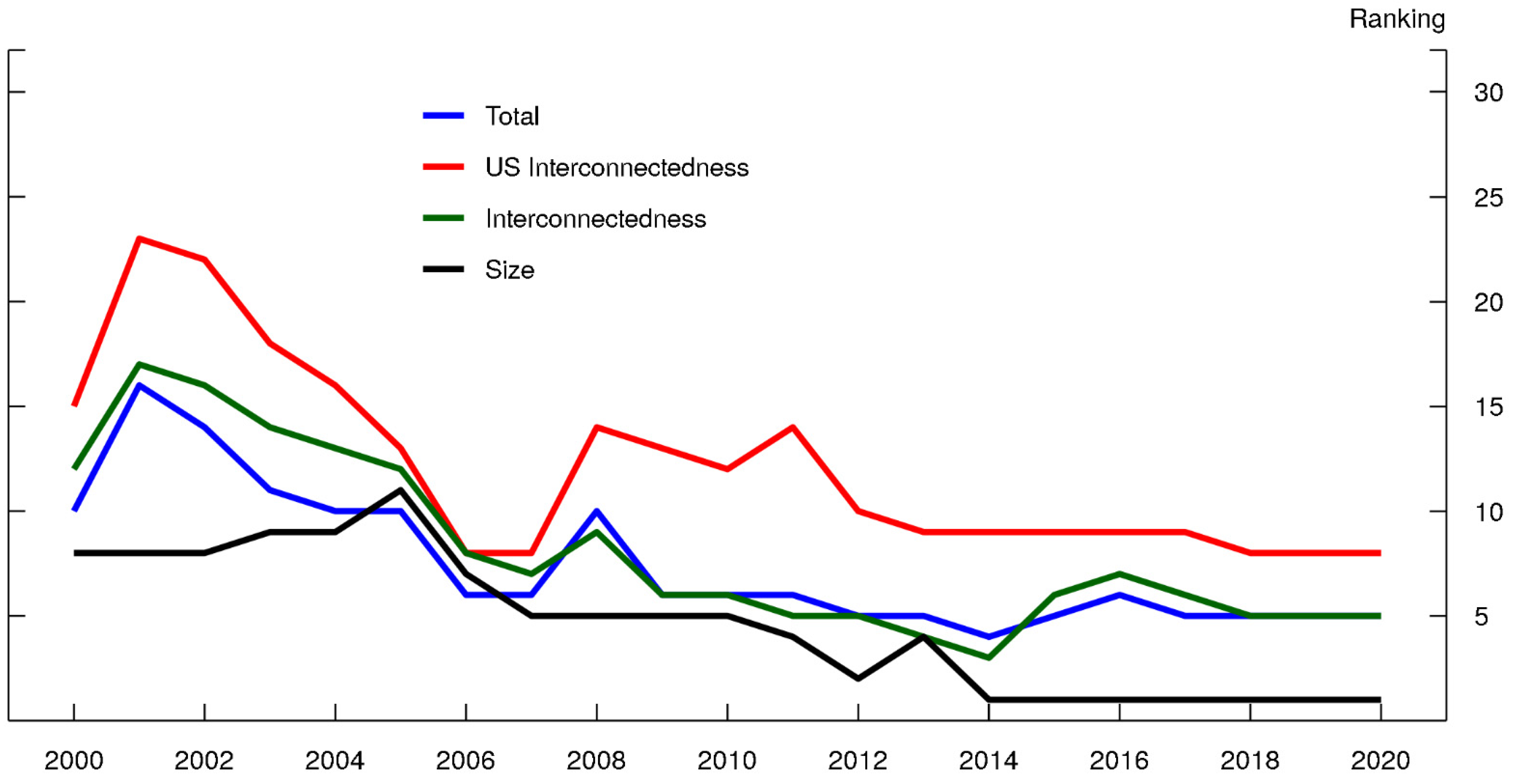
7
A financial stability event encompasses financial crises and other periods of financial stress not officially classified as crises that create notable financial disruptions.
8
To construct the rankings, we use information from the Bank for International Settlements (BIS), Bloomberg, Haver Analytics, and the International Monetary Fund (IMF). The size category is composed of a measure of real GDP, equity and bond market capitalization, and the size of the banking sector and other nonbank financial institutions. For interconnectedness we use measures of trade, foreign direct investment, and cross-border portfolio investments and bank loans.
9
If at least two of the series in the size category have observed values (i.e., are not missing) for a country in a given year, then we calculate the size ranking for that country; otherwise, we set that ranking to “missing”. For the interconnectedness and U.S. interconnectedness series, we require a minimum of four observed values to calculate the ranking for the country in a specific year. To calculate the overall ranking for a country, we require at least two categories with nonmissing rankings.
10
For U.S. banks, these bank exposures are collected in the Federal Financial Institutions Examination Council (FFIEC) 009 report, and bank capital information is aggregated using the reporting in the FFIEC 031 and FR Y-9C forms. Note that the FFIEC 009 report provides a conservative measure of exposures. Claims are only adjusted for explicit third-party guarantees, near-perfect hedges, and certain liquid collateral held outside the country of the borrower.
11
Banks in the United Kingdom have the largest exposures to China and Hong Kong (Table 2), with claims representing 181 percent of this banking sector’s Tier 1 capital.
12
Available data suggest holdings of Chinese securities represent only about 1 percent of U.S. portfolio investment, even when including securities issued through offshore affiliates (from Treasury International Capital (TIC) data by residence, adjusted to a nationality basis using the methodology of Bertaut et al. (2019)).
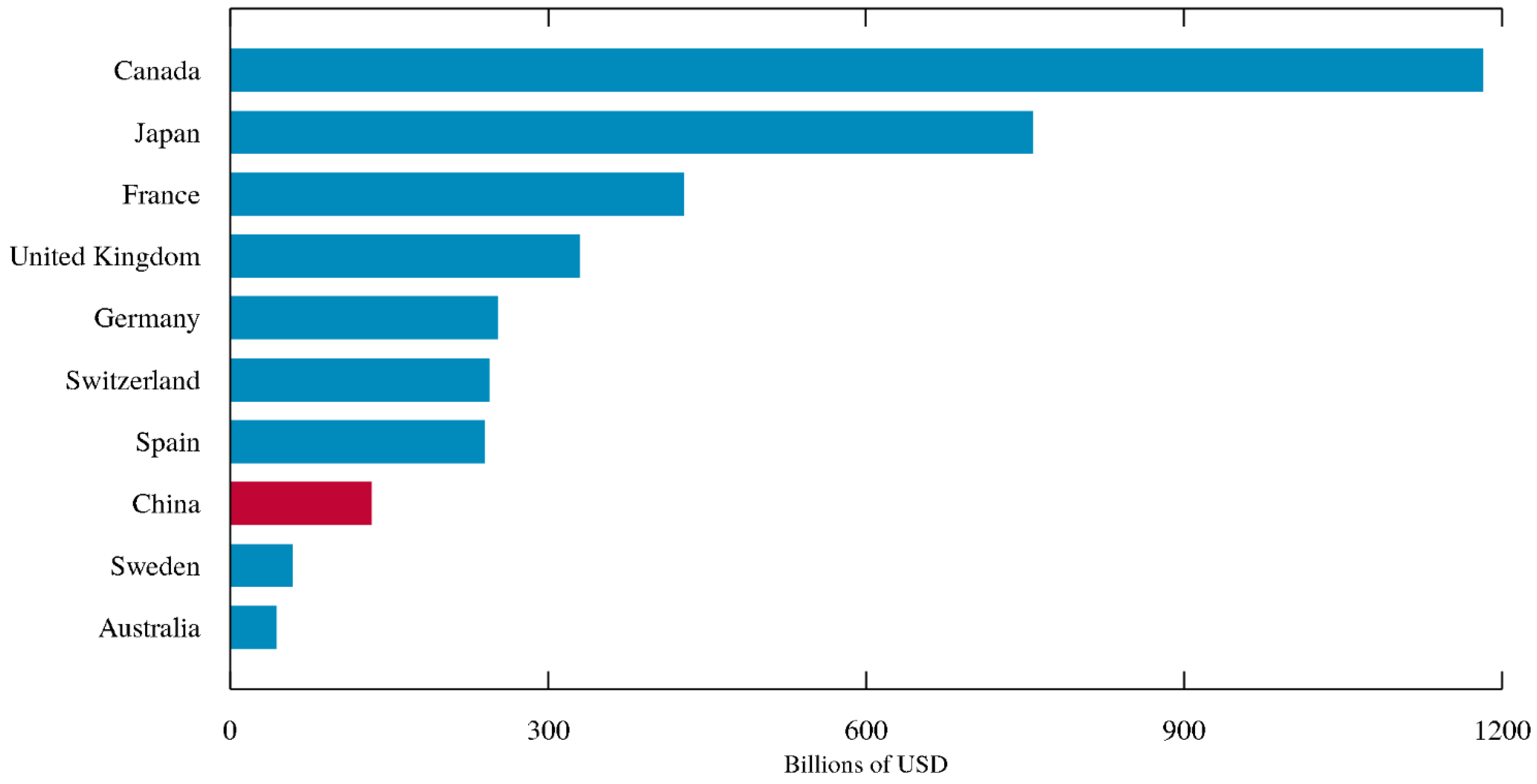
13
U.S. bank exposures to EME commodity exporters totaled almost $300 billion at the end of June 2021 (Table 4).
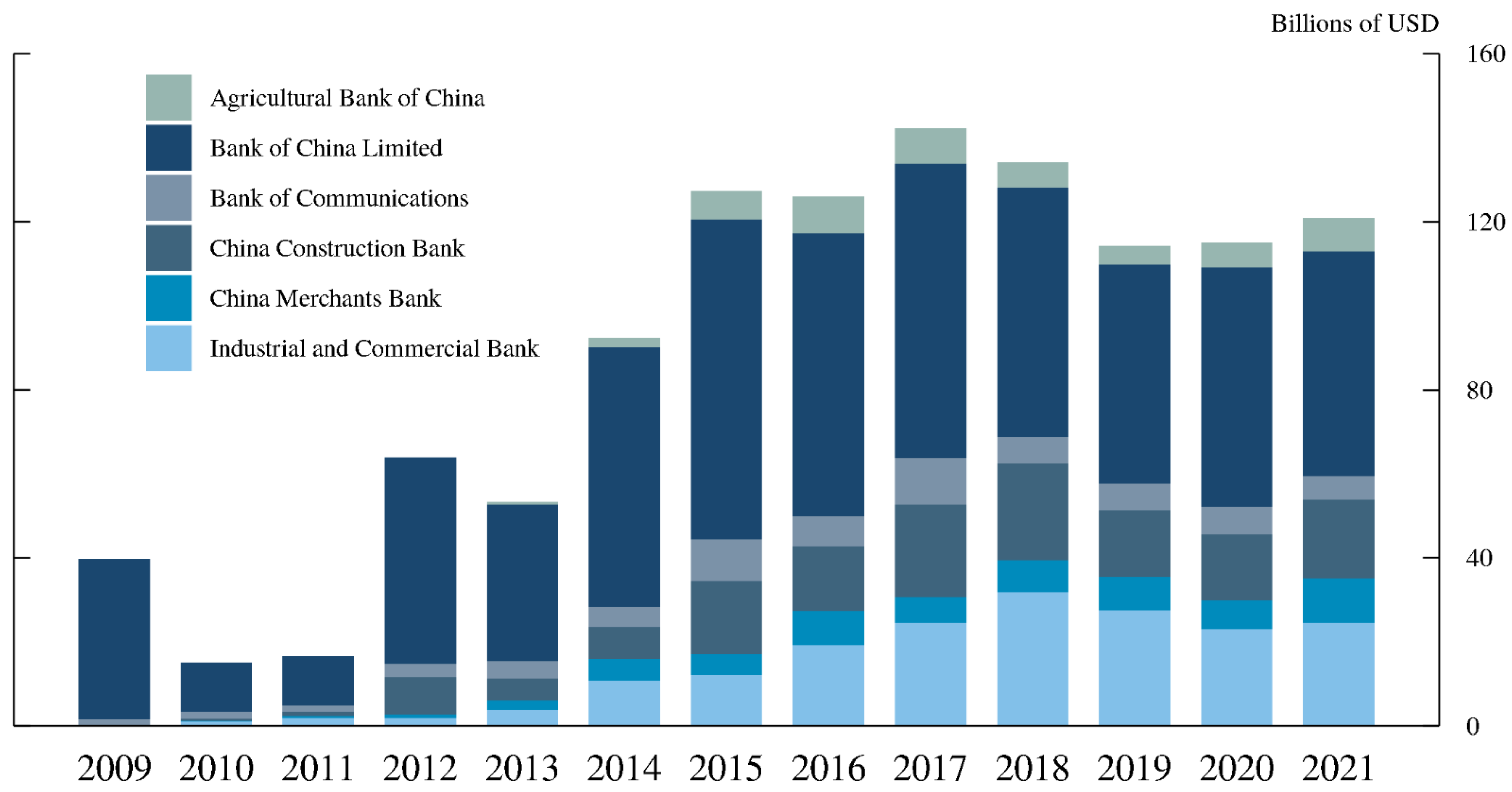
14
Money market funds’ exposure to Chinese financial institutions was $2.5 billion at the end of September 2021 (Table 5), mostly in unsecured instruments (such as time deposits).
15
We begin our sample in 2002:Q1 to avoid the structural break introduced by the entry of China into the WTO and the resulting increase in international trade. Indeed, when we extend our sample back to 1990:Q1, we find significantly smaller effects of a reduction in Chinese growth on international variables. We also end the sample period in 2017:Q4 to avoid the uncertainty generated due to the trade tensions between the United States and China and the COVID pandemic. More detailed results from this analysis are available from the authors upon request.
16
Part A of the Supplementary Materials provides a more detailed description of the VAR model and how the shocks are identified.
17
The eight global variables are ordered as follows: U.S. long-term yields, broad nominal dollar, VIX, EMBI spreads, oil prices, metals prices, G-7 economies’ GDP growth, and growth of global imports excluding Asian EMEs.
18
During the GFC, the correlation between some of the variables and China’s GDP was very strong, which translates into larger estimated effects of internally originated shocks to China’s GDP on some of the other variables (both variables analyzed in the first stage and variables analyzed in the second stage) when the GFC dummy variable is not included in the model. Results without the GFC dummy variable are available from the authors upon request.
19
For ease of exposition, we will use “China GDP shock” and “domestic China GDP shock” interchangeably throughout the rest of the paper. Unless specifically noted, we are always referring to the part of unexpected fluctuations in China’s GDP growth that can be attributed to domestic factors.
20
The confidence intervals shown in Figure 6 should be seen as a lower bound for the real size of the 90 percent confidence intervals around the estimated impulse response functions because we did not account for the fact that the China GDP shocks were estimated in the first stage. Ultimately, what these confidence intervals tell us is that the effects of a China GDP slowdown are quite uncertain, and therefore any policy response to such an event should take this high degree of uncertainty into consideration.
21
We estimate the historical impact on growth of financial crises by computing the difference between the average annualized real GDP growth in the two years before a financial crisis with the average real GDP growth in the two years after a financial crisis. The financial crisis episodes are taken from the database compiled by Reinhart and Rogoff (2011) and Laeven and Valencia (2013). These estimates exclude the most recent wave of economic recessions caused by the COVID-19 pandemic.
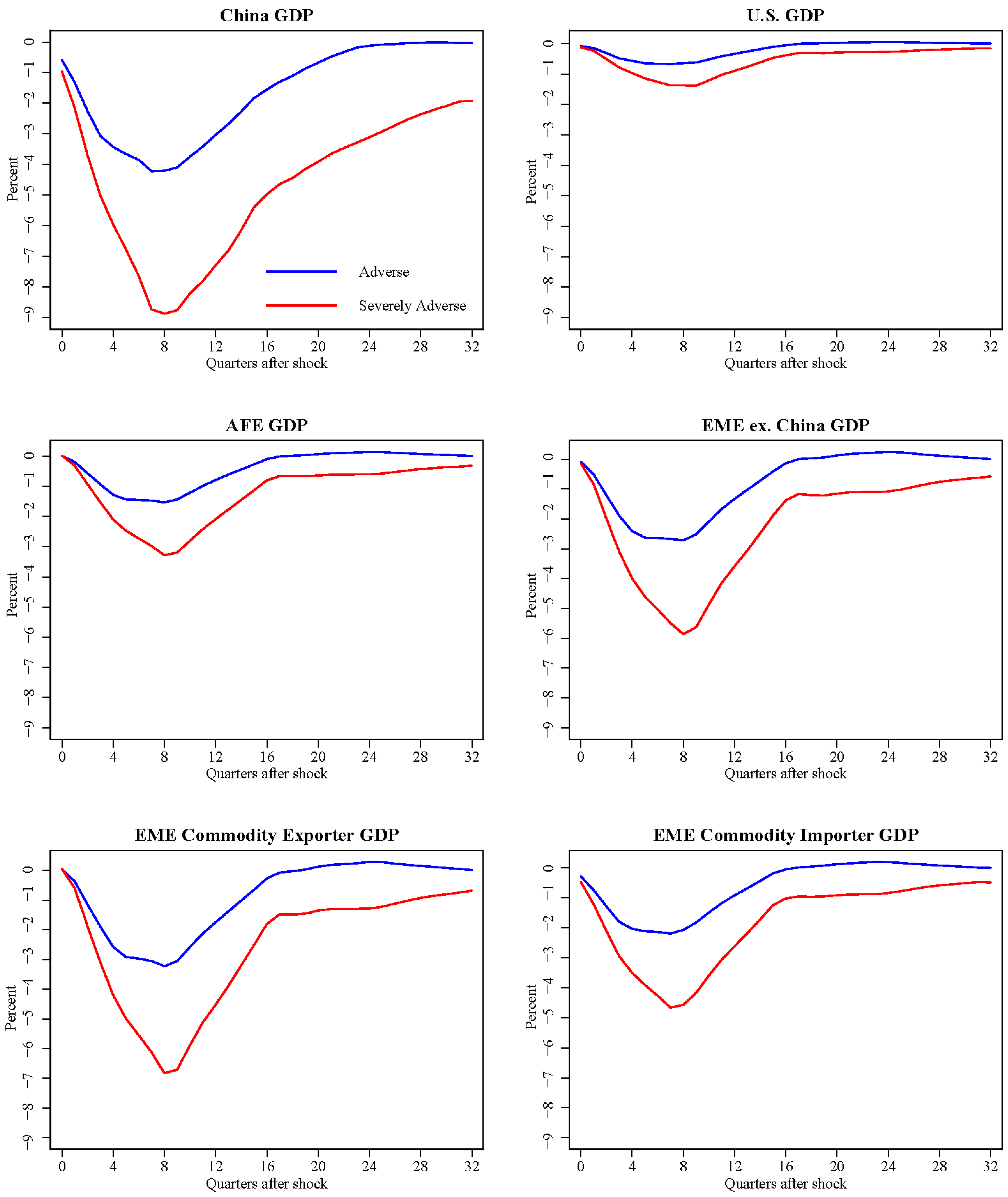
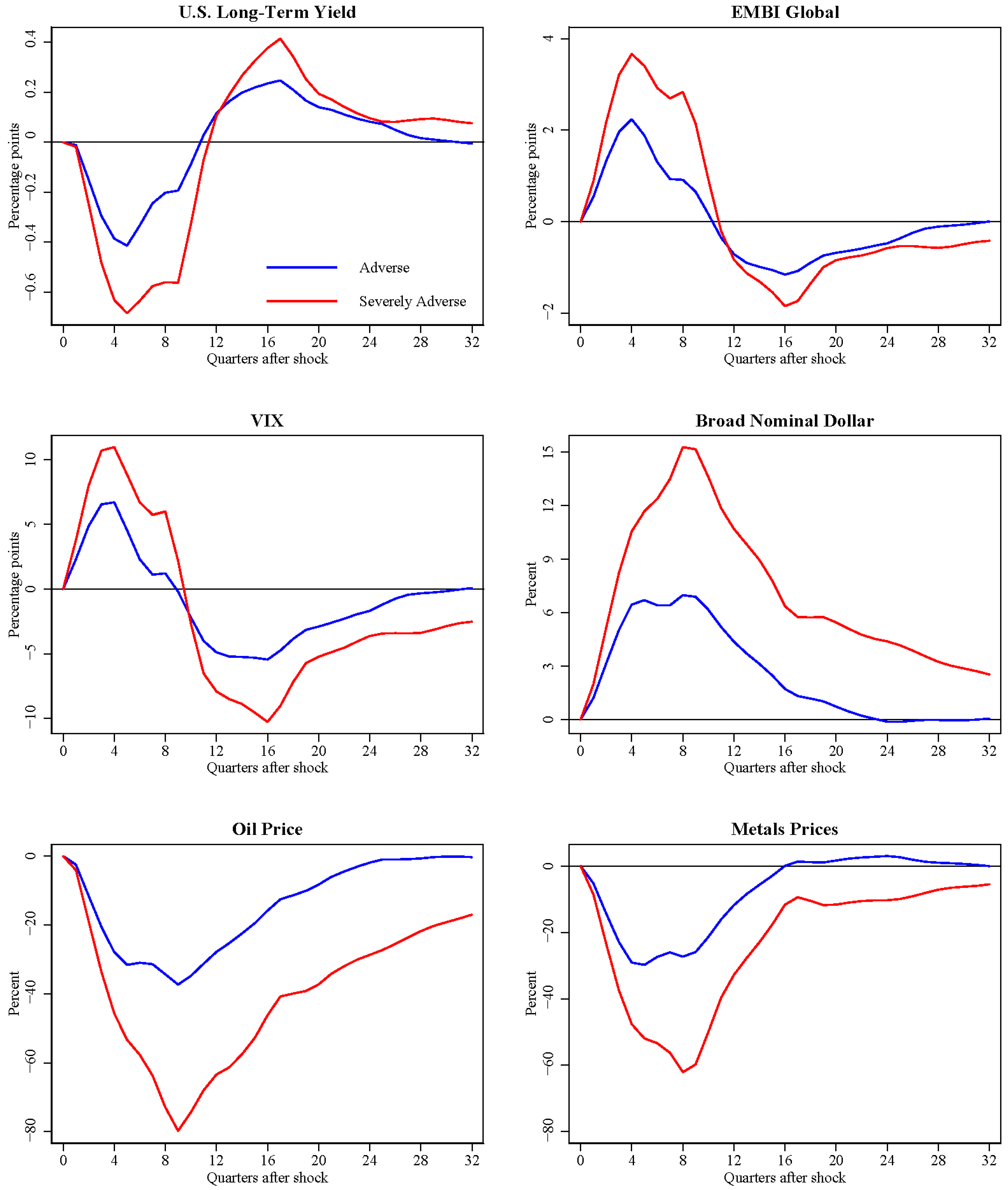
22
To obtain the sequence of shocks hitting China’s GDP that generate GDP paths such as those in the top panel of Figure 7, we use the estimated impulse response functions from the first-stage SVAR to account for the dynamic effects of the shocks in China’s GDP but also on the global variables included in the model. We also had to make the simplifying assumption that these shocks were serially uncorrelated.
23
Part B of the Supplementary Materials provides a brief summary of the SIGMA model.
24
Using price quotes from Bloomberg, we compute the market return and level changes from the previous day’s close (4 p.m. Eastern Standard Time) to the event day’s open (9 a.m. Eastern Standard Time). This uniform time horizon allows us to capture the pre-market open in China (4 a.m. China Standard Time) and post-market close (9 p.m. China Standard Time), even though the European markets and U.S. markets continue trading after the end of our event window. This timing convention is used for all assets in Table 6 except for U.S. corporate spreads, which is the previous day close (4 p.m. Eastern Standard Time) to the event day close (4 p.m. Eastern Standard Time).
25
The automatic circuit breakers led to a halting of trading for brief periods and also led, early in the day on 7 July, after a quick 7 percent decline, to a suspension of trading for the remainder of the day. The circuit breakers were later abandoned because, outside of the period when trading stood suspended, they appeared to increase volatility.
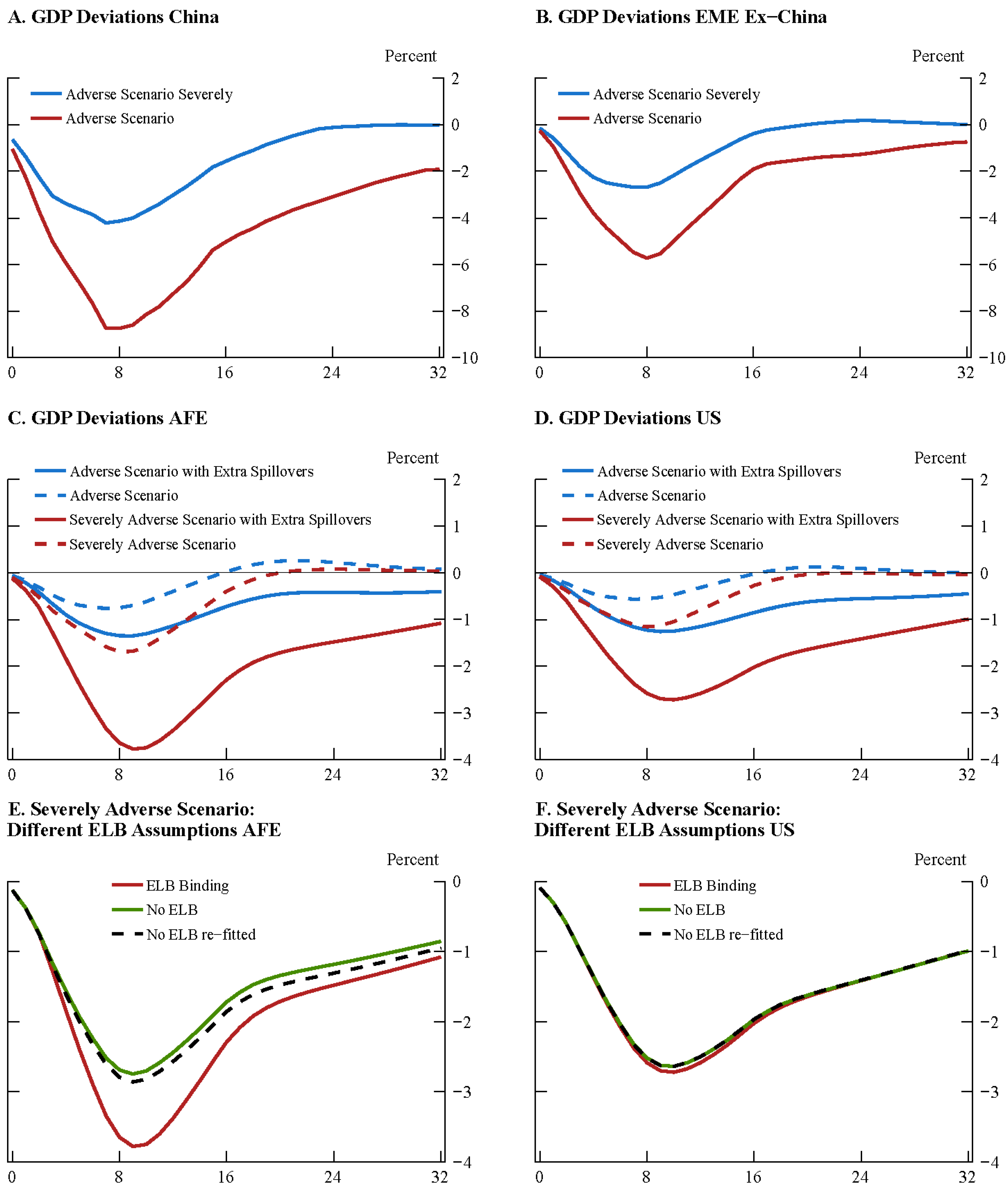
26
As the current version of SIGMA has only an aggregate EME bloc, we use the results from our SVAR to construct an overall EME GDP response to an adverse growth event in China. In each simulation, we feed in a series of shocks to the EMEs in our SIGMA model to mimic the response in each of our two Chinese adverse scenarios. Therefore, the GDP responses of the EMEs, shown in Figure 9, panels A and B, are by construction identical to the ones embedded in the SVAR analysis.
27
We also used a set of demand shocks triggered two years before the crisis begins to place the model into an initial policy rate condition similar to the world economy in mid-2018. These initial conditions are interesting as they allow for the possibility of a binding ELB in one, but not both, of the two advanced economy blocs in the simulation. All simulation results are reported as deviations from the paths implied by those initial shocks. We used data from Haver Analytics and the World Economic Outlook to construct that baseline.
28
The GDP losses occur despite an accommodative U.S. monetary policy response, which follows the model’s policy reaction function.
29
In the simulation, the ELB binds for seven quarters.

References

  1. Ahmed, Shaghil. 2017. China’s Footprints on the Global Economy: Remarks Delivered at the Second IMF and Federal Reserve Bank of Atlanta Research Workshop on the Chinese Economy; IFDP Notes. Washington, DC: Board of Governors of the Federal Reserve System, September 28. Available online: https://www.federalreserve.gov/econres/notes/ifdp-notes/chinas-footprints-on-the-global-economy-20170928.htm (accessed on 1 October 2021).
  2. Aldasoro, Iñaki, Claudio Borio, and Mathias Drehmann. 2018. Early Warning Indicators of Banking Crises: Expanding the Family. BIS Quarterly Review, 29–45. Available online: https://www.bis.org/publ/qtrpdf/r_qt1803e.pdf (accessed on 1 October 2021).
  3. Barro, Robert J. 2016. Economic Growth and Convergence, Applied Especially to China. NBER Working Paper Series 21872; Cambridge: National Bureau of Economic Research. Available online: https://www.nber.org/papers/w21872 (accessed on 1 October 2021).
  4. Bernanke, Ben, Jean Boivin, and Piotr Eliasz. 2005. Measuring the Effects of Monetary Policy: A Factor Augmented Vector Autoregressive (FAVAR) Approach. Quarterly Journal of Economics 120: 387–422. [Google Scholar]
  5. Bertaut, Carol, Beau Bressler, and Stephanie Curcuru. 2019. Globalization and the Geography of Capital Flows. FEDS Notes. Washington, DC: Board of Governors of the Federal Reserve System, September 6. [Google Scholar] [CrossRef]
  6. Buch, Claudia, and Linda Goldberg. 2015. International Banking and Liquidity Risk Transmission: Lessons from Across Countries. IMF Economic Review 63: 377–410. [Google Scholar] [CrossRef] [Green Version]
  7. Cecchetti, Stephen, Madhusudan Mohanty, and Fabrizio Zampolli. 2011. The Real Effects of Debt. BIS Working Papers No. 352. Basel: Bank for International Settlements, September, Available online: https://www.bis.org/publ/work352.pdf (accessed on 1 October 2021).
  8. Cetorelli, Nicola, and Linda Goldberg. 2012. Follow the Money: Quantifying Domestic Effects of Foreign Bank Shocks in the Great Recession. American Economic Review 102: 213–18. [Google Scholar] [CrossRef] [Green Version]
  9. Chen, Sally, and Joong Shik Kang. 2018. Credit Booms—Is China Different? IMF Working Paper No. 18/2. Washington, DC: International Monetary Fund, January, Available online: https://www.imf.org/en/Publications/WP/Issues/2018/01/05/Credit-Booms-Is-China-Different-45537 (accessed on 1 October 2021).
  10. Correa, Ricardo, Horacio Sapriza, and Andrei Zlate. 2021. Wholesale Funding Runs, Global Banks’ Supply of Liquidity Insurance, and Corporate Investment. Journal of International Economics 133: 103519. [Google Scholar] [CrossRef]
  11. Dell’Ariccia, Giovanni, Deniz Igan, Luc Laeven, and Hui Tong. 2016. Credit Booms and Macrofinancial Stability. Economic Policy 31: 299–355. [Google Scholar] [CrossRef]
  12. Dieppe, Alister, Robert Gilhooly, Jenny Han, Iikka Korhonen, and David Lodge. 2018. The Transition of China to Sustainable Growth–Implications for the Global Economy and the Euro Area. ECB Occasional Paper Series No. 206; Frankfurt: European Central Bank, January, Available online: https://www.ecb.europa.eu/pub/pdf/scpops/ecb.op206.en.pdf (accessed on 1 October 2021).
  13. Ehlers, Thorsten, Steven Kong, and Feng Zhu. 2018. Mapping Shadow Banking in China: Structure and Dynamics. BIS Working Paper No. 701. Basel: Bank for International Settlements. Available online: https://www.bis.org/publ/work701.pdf (accessed on 1 October 2021).
  14. Eichengreen, Barry, Donghyun Park, and Kwanho Shin. 2012. When Fast-Growing Economies Slow Down: International Evidence and Implications for China. Asian Economic Papers 11: 42–87. [Google Scholar] [CrossRef]
  15. Ericsson, Neil, Lucas Husted, and J. E. Seymour. 2014. Potential Spillovers of a Sudden Slowdown in China. Unpublished paper. Board of Governors of the Federal Reserve System. [Google Scholar]
  16. Erten, Bilge. 2012. Macroeconomic transmission of Eurozone shocks to emerging economies. Economie Internationale 131: 43–70. [Google Scholar] [CrossRef]
  17. European Central Bank. 2017. China’s economic growth and rebalancing and the implications for the global and euro area economies. ECB Economic Bulletin Volume 7: 32–52. [Google Scholar]
  18. Fontaine, Idriss, Laurent Didier, and Justinien Razafindravaosolonirina. 2017. Foreign policy uncertainty shocks and US macroeconomic activity: Evidence from China. Economics Letters 155: 121–25. [Google Scholar] [CrossRef]
  19. Gauvin, Ludovic, and Cyril C. Rebillard. 2018. Towards Recoupling? Assessing the Global Impact of a Chinese Hard Landing Through Trade and Commodity Price Channels. World Economy 41: 3379–415. [Google Scholar] [CrossRef] [Green Version]
  20. Gilhooly, Robert, Jen Han, Simon Lloyd, Niamh Reynolds, and David Young. 2018. From the Middle Kingdom to the United Kingdom: Spillovers from China. In Quarterly Bulletin 2018 Q2. London: Bank of England. Available online: https://www.bankofengland.co.uk/quarterly-bulletin/2018/2018-q2/from-the-middle-kingdom-to-the-united-kingdom-spillovers-from-china (accessed on 1 October 2021).
  21. Hsieh, Chang-Tai, and Peter J. Klenow. 2009. Misallocation and Manufacturing TFP in China and India. Quarterly Journal of Economics 124: 1403–48. [Google Scholar] [CrossRef]
  22. Huang, Zhuo, Chen Tong, Han Qiu, and Yan Shen. 2018. The Spillover of Macroeconomic Uncertainty between the U.S. and China. Economic Letters 171: 123–27. [Google Scholar] [CrossRef]
  23. Laeven, Luc, and Fabian Valencia. 2013. Systemic Banking Crises Database. IMF Economic Review 61: 225–70. [Google Scholar] [CrossRef] [Green Version]
  24. Lee, Jong-Wha, and Kiseok Hong. 2010. Economic Growth in Asia: Determinants and Prospects. Asian Development Bank Economics Working Paper Series, (220); Mandaluyong: Asian Development Bank. [Google Scholar]
  25. Lee, Seung J., Kelly E. Posenau, and Viktors Stebunovs. 2020. The Anatomy of Financial Vulnerabilities and Banking Crises. Journal of Banking and Finance 112: 105334. [Google Scholar] [CrossRef]
  26. Li, Cindy. 2016. The Changing Face of Shadow Banking in China. Asia Focus. San Francisco: Federal Reserve Bank of San Francisco, December, Available online: https://www.frbsf.org/banking/wp-content/uploads/sites/5/Asia-Focus-The-Changing-Face-of-Shadow-Banking-in-China-December-2016.pdf (accessed on 1 October 2021).
  27. Li, Jianjun, Sara Hsu, and Yanzhi Qin. 2014. Shadow Banking in China: Institutional Risks. China Economic Review 31: 119–29. [Google Scholar] [CrossRef] [Green Version]
  28. Ma, Guonan, Ivan Roberts, and Gerard Kelly. 2017. Rebalancing China’s Economy: Domestic and International Implications. China & World Economy 25: 1–31. [Google Scholar]
  29. Manu, Ana-Simona, Peter McAdam, and Alpo Willman. 2018. The Role of Factor Substitution and Technical Progress in China’s Great Expansion. ECB Working Paper No. 2180. Frankfurt: European Central Bank, September, Available online: https://www.ecb.europa.eu/pub/pdf/scpwps/ecb.wp2180.en.pdf (accessed on 1 October 2021).
  30. McCauley, Robert N., and Chang Shu. 2019. Recent renminbi policy and currency co-movements. Journal of International Money and Finance 95: 444–56. [Google Scholar] [CrossRef]
  31. Pang, Ke, and Pierre L. Siklos. 2016. Macroeconomic Consequences of the Real-Financial Nexus: Imbalances and Spillovers between China and the U.S. Journal of International Money and Finance 65: 195–212. [Google Scholar] [CrossRef] [Green Version]
  32. Perry, Emily, and Florian Weltewitz. 2015. Wealth Management Products in China; Bulletin, June Quarter. Sydney: Reserve Bank of Australia, pp. 59–67. Available online: https://www.rba.gov.au/publications/bulletin/2015/jun/pdf/bu-0615-7.pdf (accessed on 1 October 2021).
  33. Plagborg-Møller, Mikkel, and Christian K. Wolf. 2021. Local Projections and VARs Estimate the Same Impulse Responses. Econometrica 89: 955–80. [Google Scholar] [CrossRef]
  34. Pritchett, Lant, and Larry H. Summers. 2014. Asiaphoria Meets Regression to the Mean. NBER Working Paper Series 20573; Cambridge: National Bureau of Economic Research, October, Available online: https://www.nber.org/papers/w20573 (accessed on 1 October 2021).
  35. Reinhart, Carmen, and Kenneth Rogoff. 2011. From Financial Crash to Debt Crisis. American Economic Review 101: 1676–706. [Google Scholar] [CrossRef] [Green Version]
  36. Song, Zheng, Kjetil Storesletten, and Fabrizio Zilibotti. 2011. Growing Like China. American Economic Review 101: 196–233. [Google Scholar] [CrossRef]
Figure 1. Financial vulnerabilities. * This narrow definition of government debt includes central government debt and explicit local government debt recognized in the national audit in 2015 but does not include off-budget borrowing after 2015. ** Off-budget fiscal debt includes local government financing vehicles and other off-budget activity. The sum of this item and recognized fiscal debt equals IMF’s definition of augmented fiscal debt. Sources: People’s Bank of China, National Bureau of Statistics, Bank for International Settlements, and IMF’s Financial Sector Assessment Program.
Jrfm 15 00596 g001
Figure 2. China’s systemic importance ranking. Sources: authors’ calculations based on information from the Bank for International Settlements, the IMF, and the World Bank.
Jrfm 15 00596 g002
Figure 3. U.S. branch assets of Chinese banks. Source: U.S. Federal Reserve Board. Data reported for Q1 of each year.
Jrfm 15 00596 g003
Figure 4. U.S. branch assets of foreign banking organizations as of End-2020. Source: Responses to FFIEC 002 reporting form.
Jrfm 15 00596 g004
Figure 5. Responses to a negative unit domestic China GDP Shock. * Noncumulative response. Note: the dashed lines represent the upper and lower bounds of the 90% confidence interval around the impulse response estimate. Source: authors’ calculations using data from Haver Analytics and Bloomberg.
Jrfm 15 00596 g005
Figure 6. Activity responses to a negative unit domestic China GDP shock. Note: the dashed lines represent the upper and lower bounds of the 90% confidence interval around the impulse response estimate. Source: authors’ calculations using data from Haver Analytics and Bloomberg.
Jrfm 15 00596 g006
Figure 7. Activity responses to China GDP scenarios. Source: authors’ calculations using data from Haver Analytics and Bloomberg.
Jrfm 15 00596 g007
Figure 8. Financial responses to China GDP scenarios. Source: authors’ calculations using data from Haver Analytics and Bloomberg.
Jrfm 15 00596 g008
Figure 9. GDP simulation results from SIGMA. Source: authors’ calculations.
Jrfm 15 00596 g009
Table 1. U.S. bank claims to China and Hong Kong *.
ChinaHong KongChina and Hong Kong
In USD Billions **13989228
As Percent of Tier 1 Capital9.86.216.0
* Exposure subtracts claims guaranteed by or collateralized by claims on residents of other countries and adds claims on residents of other countries that are guaranteed by or collateralized by claims on local residents. ** Total exposure is equal to the sum of cross-border claims, foreign office claims, and derivatives. Sources: BIS consolidated banking statistics, IMF FSI, FFIEC 031, FR Y-9C, and authors’ calculations. As of 2021:Q2.
Table 2. Banks’ exposures to China and Hong Kong *.
USD BillionsPct. of Tier 1
United Kingdom767180.5
Singapore **237
United States22816
Japan17124.6
France9320.4
* Banking systems exposures are the sum of cross-border and foreign office exposures of banks headquartered in countries that compile the BIS consolidated banking statistics. Claims are adjusted for explicit third-party guarantees, near-perfect hedges, and certain liquid collateral held outside the country of the borrower. ** Singapore does not report Tier 1 data. Sources: BIS consolidated banking statistics, IMF FSI, FFIEC 031, FR Y-9C, and authors’ calculations. As of 2021:Q2.
Table 3. U.S.-headquartered banks’ exposure to banks in *.
USD BillionsPct. of Tier 1
United Kingdom372.6
Singapore80.6
Japan986.9
France332.3
* Banking systems exposures are the sum of cross-border and foreign office exposures of banks headquartered in countries that compile the BIS consolidated banking statistics. Claims are adjusted for explicit third-party guarantees, near-perfect hedges, and certain liquid collateral held outside the country of the borrower. Sources: BIS consolidated banking statistics, IMF FSI, and authors’ calculations. As of 2021:Q2.
Table 4. U.S. banks’ exposures to EME commodity exporters.
Commodity ExportersUSD Billions
Mexico109
Brazil86
Saudi Arabia22
Malaysia18
Russia16
Indonesia14
Chile9
Argentina7
Colombia7
Total287.0
Sources: FFIEC 009 and FFIEC 009a. As of 2021:Q2.
Table 5. Exposures of U.S. MMFs to China.
Panel A: By Issuer Type
IssuerTotal MMF Exposure (USD Billions)By Instrument TypeBy MaturityHolding WAM (Days)
(USD Billions)(USD Billions)
CPCDsTime DepositsO/N2–7 Days8–30 Days>30 Days
China Total2.50.60.51.50.91.20.2192.0--
Banks Subtotal2.40.50.51.50.91.20.1192.0--
Industrial & Commercial Bank of China0.30.20.00.10.30.00.001
China Construction Bank Corporation0.60.20.40.00.10.30.17512
Agricultural Bank of China1.50.10.11.40.50.90.01178
Bank of China0.00.00.00.00.00.00.0015
Other Financial Subtotal0.10.10.00.00.00.00.10.0--
COFCO Capital Corporation0.10.10.00.00.00.00016.0
Panel B: By U.S. Mutual Fund Complex
ComplexTotal Exposure (USD Billions)By Security TypePct. Of Complex AUMPct. Of Complex Prime AUMMaximum Pct. Of Fund AUMExposure WAM (Days)
(USD Billions)
CPCDsTime Deposits
Goldman Sachs0.00.00.00.00.00.40.46
Invesco0.30.20.10.00.37.96.941
JP Morgan2.00.30.31.50.42.41.73
Legg Mason0.10.00.10.00.10.60.812
Wells Fargo0.10.10.00.00.00.91.016
Note: May not sum to total due to rounding. Source: SEC Form NPF, as of 30 September 2021.
Table 6. Percent of forecast error attributable to China GDP by number of quarters.
HorizonU.S. Long-Term YieldBroad Nominal DollarVIXEMBI GlobalOil PriceMetals PriceG7 GDPWorld Trade ex. EME AsiaChina GDP
1 79.9
20.011.37.38.71.413.13.77.565.3
34.314.06.718.69.217.47.88.960.4
47.513.47.322.99.016.77.810.256.8
87.614.59.320.89.417.78.911.549.1
127.814.79.321.19.717.89.411.848.8
7.814.79.421.09.717.89.511.948.3
Source: authors’ calculations using data from Haver Analytics and Bloomberg.
Table 7. Percent of forecast error attributable to China GDP by number of quarters.
HorizonChina GDPU.S. GDPAFE GDPEME ex. China GDPEME Commodity Exporter GDPEME Commodity Importer GDP
179.90.70.00.90.15.9
265.30.76.410.113.56.5
360.41.99.615.921.36.9
456.81.99.615.821.46.8
849.12.09.716.421.76.9
1248.82.09.716.421.76.9
48.32.09.716.421.76.9
Source: authors’ calculations using data from Haver Analytics and Bloomberg.
Table 8. Market reactions during China event windows in 2015–2016.
Market Reaction *Historical Percentiles
Event #1 11 August 2015Event #2 ** 24 August 2015Event #3 ** 4–7 January 20161% Tail5% TailMost Extreme Value
Broad Dollar0.70%−0.10%1.30%0.65%0.40%1.62%
Broad AFE0.10%−0.90%0.50%0.92%0.56%1.95%
Broad EME1.20%0.50%1.90%0.59%0.38%2.24%
U.S. 2Y yield−4.8−5.7−8.8−5.7−2.8−15.4
U.S. 10Y−6.4−7.5−10.8−9.8−6.2−19.9
German 10Y−4.2−0.3−10.1−9.4−5.8−23.8
U.K. 10Y−5.78−16.5−11.1−7.1−29.7
Japan 10Y−1.4−1−2.4−4.8−2.8−12.7
S&P 500 Futures−0.6%−3.8%−4.5%−1.8%−1.0%−3.8%
EuroSTOXX−1.4%−4.5%−6.4%−2.8%−1.6%−7.7%
FTSE 100−0.8%−4.0%−5.4%−2.2%−1.3%−5.1%
MSCI EM−0.4%−4.3%−5.8%−2.9%−1.5%−7.3%
VIX1.014.73.72.601.256.55
VDAX2.259.58.063.672.029.49
US Corp Spread 2.93.74.69.214.5635.05
EMBI+ Spread8131515828
* Overnight change as of close (4pm EST) to open (9am EST) the next day for exchange rate indices, equity markets, VIX, VDAX, and government bond indices. The 1-day change as of close to close for US corporate spread and EMBI+. ** Event falls on Monday, change as of previous Friday close to Monday open. Event 4 is the cumulative change over four days. Source: Bloomberg.
Publisher’s Note: MDPI stays neutral with regard to jurisdictional claims in published maps and institutional affiliations.

