What Microeconomic Fundamentals Drove Global Oil Prices during 1986–2020?

Abstract

The global financial crisis of 2007–2009 caused major economic disturbances in the oil market. In this paper, we consider five variables that describe the microeconomics of the supply of and demand for oil, and evaluate their importance before, during and after the global financial crisis. We consider five dissimilar regimes during the period of January 1986 to the end of 2020: two regimes prior to the global financial crisis, the regime during the crisis, and two regimes after the crisis. The main hypothesis tested is that oil fundamentals of supply and demand remained important, even though the five regimes were dissimilar. We built five boosted and over-fitted neural networks to capture the exact relationships between spot oil prices and oil data related to these prices. This analysis shows that, while the inputs into an accurate neural network can remain the same, the impact of each variable can change considerably during different regimes.

1. Introduction

Global oil markets are complex, and the price of oil exhibits significant volatility. During the past four decades, the price of oil was as low as about USD 20 in the late 1990s and as high as USD 150 before the global financial crisis. Baumeister and Kilian (2016) conducted an excellent overview of the behavior of oil prices over the past forty years, with a special focus on the fluctuations of these prices. They emphasized that fluctuations of such magnitude contain a large component of surprise, in the sense that ordinary economic foresight could not penetrate the dynamic succession of regime shifting in oil markets. For example, events such as the 1973–1974 oil crisis, which saw deliberate cuts in oil production in Arab OPEC countries, were followed by the unexpected period of Great Moderation during the mid-1980s.

The moderation of inflation and the reduction of real GDP fluctuations created conditions for increased risk-taking and the housing bubble of 2002 to 2007, which was characterized by an associated global boom in emerging markets such as China, India and Brazil that fueled big increases in the price of oil. Then, the world experienced the unforeseen global financial crisis (GFC) and the ushering in of unconventional monetary policies around the world, which brought oil prices from about USD 150 down to USD 40.

The post-crisis period during 2009 to 2013 recorded steady increases in the price of oil, from a low of about USD 40 to a high of USD 110, primarily because of the economic recovery of the global economy. The most recent period, from June 2013 to December 2020, shows how U.S. fracking technology, with its strong shale production, combined with rising OPEC output and slowing demand from China, have contributed to dramatic declines in oil prices, from a high of USD 100 in June 2014 to a low of USD 30 in February 2016. During the 2016–2020 period, oil prices fluctuated between a low of USD 30 in February 2016 to a high of USD 75 in September 2018, to drop again to USD 20, one of oil’s lowest prices, during April 2020, when the COVID-19 crisis destabilized the entire global economy.

Baumeister and Kilian (2014, 2015, 2016) carried out a comprehensive analysis of this period, while other authors have examined specific topics and periods, such as Hamilton (1983); Bernanke et al. (1997); Nakov and Pescatori (2010); Kilian (2008).

The focus of this paper is the pricing of oil and its determinants. We consider five variables that describe the microeconomics of the supply of, and demand for oil, motivated by a similar approach proposed by Kilian (2009). We evaluate their importance as oil determinants and their variability before, during, and after the GFC. We consider five dissimilar regimes during the period of January 1986 to the end of 2017: two regimes prior to the global financial crisis, the regime during the crisis, and two regimes after the crisis. Malliaris and Malliaris (2020) studied the behavior of the global price of oil using macroeconomic variables and employing the methodology of overlapping regressions. Bhar et al. (2021) focused on U.S. oil production.

The classic paper on regime changes is Ang and Timmermann’s (2012), which instructs us about the methodology used. Economists are familiar with two regime methodologies from the analysis of business cycles. One regime contains periods of economic growth and the next regime includes periods of decline. The fundamental assumption is that all regimes of growth are similar in all other respects; the same is assumed for regimes of decline. However, regimes need not repeat themselves between just the two states of growth and decline.

Most techniques consider two regimes, and in the case of oil, these have been applied extensively in papers such as Bhar and Malliaris’s (2011) and Tsai’s (2015). Related papers are Noguera’s (2013); Salisu and Fasanya’s (2013); Xiong et al.’s (2013). In our case, we identify five regimes, described in Section 2, and assume that each such regime is distinctive.

The main hypothesis tested is that the oil fundamentals of supply and demand remain important even though the five regimes are dissimilar. We build five boosted and over-fitted neural networks to capture the exact relationships between spot oil prices and oil data related to those prices. Overfitting involves letting the model train on a specific data set until it fits that data very closely. Such a model cannot generalize well to other datasets, but can explain one specific set well. This analysis shows that, while the inputs into an accurate neural network can remain the same, the impact of each variable can change considerably during different regimes. We find that the shifts in impacts of the various inputs are great enough to support the hypothesis that there are important structural breaks between periods.

There are many reasons to avoid overfitting a neural network, particularly because it destroys any chance of building a generalized model that will be suitable over time. However, in this paper, we use the downsides of overfitting to our benefit. By overfitting models of five different time periods, we are able to highlight why generalization is difficult over the entire period. By building, then comparing, five bespoke networks, we can identify the specific areas where general models will need to improve in order to forecast well. Although we do not perform any forecasting, the neural network methodology applied in this paper, the microeconomic data of the independent inputs used, and the results obtained provide an excellent impetus for further work in this area along the lines of Chen’s (2014); Jammazi and Aloui’s (2012) and Shin et al.’s (2013).

In this paper, we build five neural network models and overfit them in order to capture the relationships among the inputs in the ways that most perfectly match their configurations in a specific period. As indicated, it is not our purpose to build forecasting models with validation sets. Rather, we want to create descriptive models that encapsulate existing relationships in different regimes of the data set. This will help us to understand shifts in variable impact over the various regimes.

2. Data

The data for this study comprise inputs related to oil and supply and demand for oil. There are five variables: the spot price of oil, the stored stocks of oil except for that held by the government as strategic petroleum reserves, net imports of oil, oil production, and product supplied. The US Energy Information Administration (EIA) uses product supplied as a representation for the amount of petroleum products consumed. All data are monthly, rather than seasonally adjusted, and were downloaded from the EIA. They cover the time period from January 1986 through to the end of 2020.

Table 1. Variables and their sources.

Variable	Data Source	Short Name	Source URL
Production of Oil in the U.S.	MCRFPUS1 from EIA	Prod	https://www.eia.gov/dnav/pet/pet_crd_crpdn_adc_mbbl_m.htm (accessed on 14 March 2021)
Net Imports of Oil in the U.S.	MTTNTUS2 from EIA	NetImp	https://www.eia.gov/dnav/pet/hist/LeafHandler.ashx?n=PET&s=MTTNTUS2&f=M (accessed on 14 March 2021)
Oil Stocks excluding the Strategic Petroleum Reserve	MTESTUS1 from EIA	Stks	https://www.eia.gov/dnav/pet/hist/LeafHandler.ashx?n=PET&s=MTESTUS1&f=M (accessed on 14 March 2021)
Product Supplied (Consumption) of Oil	MTTUPUS1 from EIA	Con	https://www.eia.gov/dnav/pet/pet_cons_psup_dc_nus_mbbl_m.htm (accessed on 14 March 2021)
Spot Price of Cushing Oil	RWTC from EIA	SpotPr	https://www.eia.gov/dnav/pet/pet_pri_spt_s1_m.htm (accessed on 14 March 2021)
Month of the year	Derived from data above	Month

gives the source of the data for each of these variables, and the abbreviated name used in the models.

The spot price of oil is the price of a single transaction for delivery of a determined quantity of oil to a specified place. Demand for oil does not change rapidly, but is seasonal. As demand varies, we see its effects on production, on imports, and on the amount of oil in storage. The stocks of oil, excluding the strategic petroleum reserves, includes the inventories stored for future use, and is reported in thousands of barrels on the last day of the week. The strategic petroleum reserve is an amount of stock maintained by the government for use during any period where there is a major disruption in supply. The values of net imports are measured in thousands of barrels imported, and include oil from the 50 states, the District of Columbia, and U.S. possessions and territories. Net imports is the amount of imports minus the amount of exports. Production is measured in thousands of barrels. Production covers the volume of oil produced from U.S. oil reservoirs. It includes the volume from the point of custody transfer to trucks, pipelines, or other means, with the intent to be transported to refineries. The quantities are estimated by the state and summed to the Petroleum Administration district (PADD) and then to the U.S. level. The Product Supplied is used as a stand-in for the consumption of petroleum products, since it is calculated as the amount of petroleum products removed from principal origins. These five variables form the fundamentals of supply: production, plus net imports, plus oil stock (inventory) and oil demand, which all determine the price of oil in the U.S. Variables were then scaled to be between zero and one. This set of variables includes the abbreviation of the original variable name followed by Scld. Scaling allows the model to treat the variables on a more equal basis, but all values will be positive, as they refer to quantities and prices. Scaling the data to be between 0 and 1, referred to as Feature Scaling in machine learning (ML), is an important process, especially when neural networks are being used. Because neural network algorithms use gradient descent as a process, they will have a better and more rapid convergence to the target when feature scaling has been used. With ML algorithms that calculate distances, larger valued attributes can dominate the output because the algorithm is affected by the relative sizes of the variables. Thus, scaling the variables speeds up the learning phase in a neural network feedforward back propagation algorithm, and helps prevent variables with large ranges from over-weighting node connections for variables with smaller ranges (Han et al. (2012); Guidici (2003); Weiss and Indurkhya (1998)). The target for each network was the scaled value of the spot price of oil.

The data set was split into five parts using the structural breaks created by the intervening economic crisis. These five time periods are shown in

Table 2. Data set time periods.

Regime	Begin	End	Number of Months
Pre-Bubble	January 1986	December 2001	180
Bubble Forming	January 2001	November 2007	83
Crisis	December 2007	May 2009	18
After Crisis	June 2009	May 2013	48
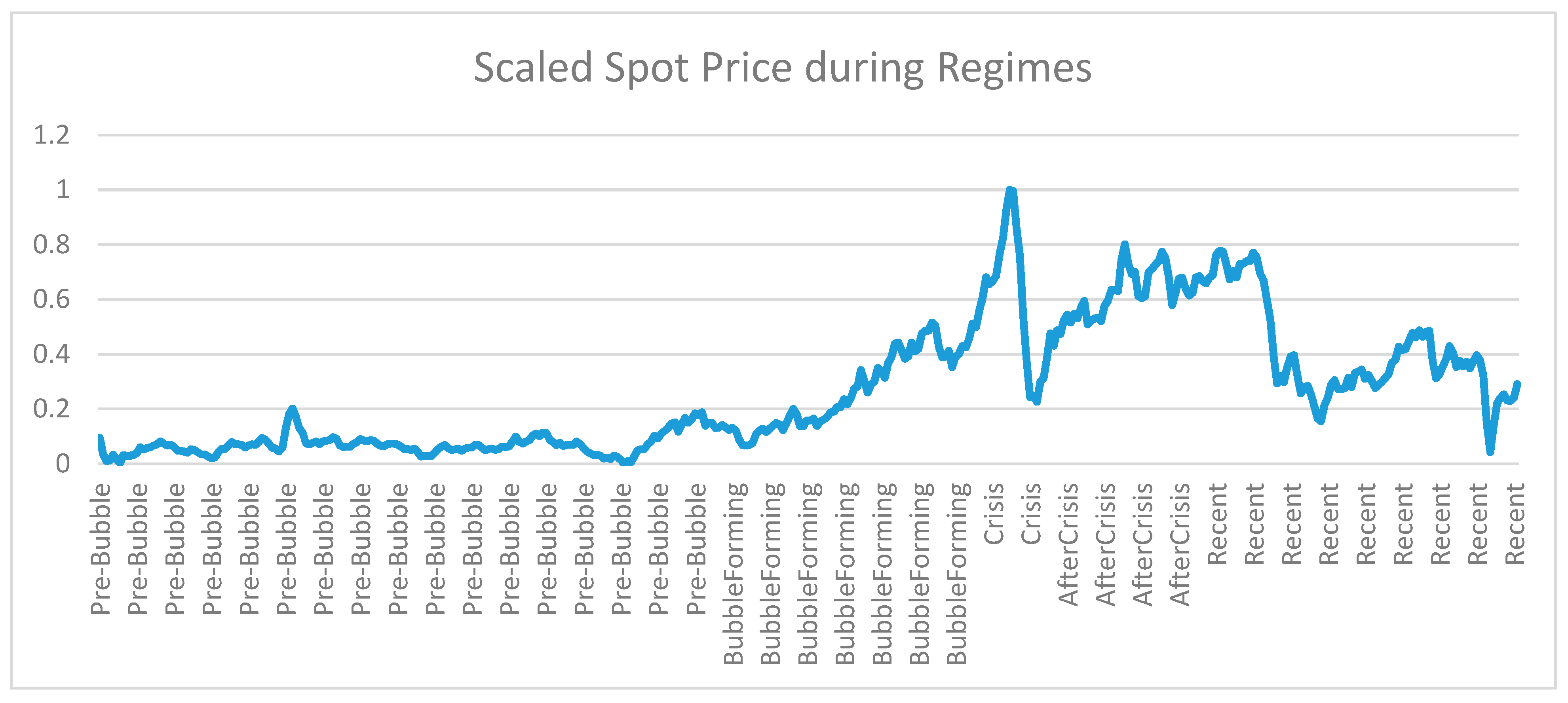
Recent	June 2013	December 2020	91

, along with the beginning and ending dates, and the number of months involved. Our entire data set begins in January of 1986 and shows a sideways movement of spot prices until late 2001, followed by a steady growth of spot prices, with some noise, until late 2007. The crisis period is the one determined by the National Bureau of Economic Research and coincides with the Great Recession that began in December 2007 and ended in May/June 2009. During this period, the oil bubble continued to grow in late 2007 and early 2008, and then collapsed with Lehman Brothers’ bankruptcy in mid-September 2008. A small bounce at the bottom led eventually to a resumption in the steady growth of prices after mid-2009. After this time period, we see another sharp downward trend, followed by a slight upward move. Thus, the middle regime is chosen objectively, since it describes the period of the Great Recession, while the two regimes before it, and the two after it, are decided by subsets that differ in terms of price volatility. Viewed together, these five regimes are dissimilar in terms of the economic conditions driving the oil market.

We used economic reasoning to characterize the subdivisions proposed. Our economic reasoning was driven by a careful and realistic assessment of important developments in the global oil market. The five periods chosen and described as: Pre-Bubble, Bubble Forming, Crisis, After Crisis, and Recent, were determined by starting with the well-defined period called the Global Financial Crisis. There is much consensus that this period started in December 2007 and ended in May 2009. Using this period as an anchor, we chose a pre-crisis and a post crisis period, and further analysis of these two broad categories guided us towards subdividing each of these into two, because numerous authors we cite in the paper have described the emergence of pre-crisis bubbles as well as post-crisis developments in fracking. This paper’s claim is: by proposing five economic regimes and building five boosted and over-fitted neural networks to capture the exact relationships between spot oil prices and oil data related to those prices, we will receive more insightful results than if we had just analyzed a single period. This analysis shows that, while the inputs into an accurate neural network can remain the same, the impact of each variable can change considerably during different regimes, and the insights from our specific regimes are more useful than the results from the whole sample period. We do not claim that we have proposed the most optimal five regimes among all possible combinations.

Support for our approach is provided by studies such as Balcilar and Ozdemir’s (2013) and Zhu et al.’s (2017). Balcilar and Ozdemir (2013) investigated the regime-switching causal nexus between U.S. oil and equity markets. The data used were the log returns of monthly crude oil futures contracts traded on the New York Mercantile Exchange and a sub-grouping of the S&P500 index. Their sample period covered the 1991 to 2011 period, which includes several important developments in the oil sector. These include the Gulf Crisis in 1991, the Asian financial crises in 1997–98, the 9/11 Terrorist Attack in 2001, the second Gulf War in 2003, and finally, the global financial crisis in 2007–9. The authors derived four regimes and studied relationships between the price of oil and equity markets.

Zhu et al. (2017) considered the impact of oil supply and demand shocks on stock returns during the period of 1985 to 2015, using a two-regime Markov regime-switching model. Unlike Balcilar et al., Zhu et al. examined the asymmetric effects of oil supply and demand shocks on stock returns in high- and low-volatility states. Their two-regime Markov regime-switching model lends support to the underlying asymmetric responses of stock returns to oil supply and demand shocks for both oil-importing and oil-exporting countries. Our use of five regimes is inspired by both Balcilar et al. and Zhu et al., who offer empirical evidence that regimes differ, and thus focusing on a number of regimes will enrich our understanding. While they applied a two-regime Markov methodology, we apply in this paper a neural network methodology, and our data are extended to include oil data during the period of 2016 to 2020. Increasing the number of regimes substantially beyond 5, say to 10 or 15, dilutes the impact of the major events that occur in markets, and diminishes the ability to reach meaningful conclusions. Simply put, too much detail may obscure critical relationships.

Figure 1 shows this graphically, along with the five periods. In Figure 2, Figure 3, Figure 4 and Figure 5, graphical representations of each of the scaled input variables are depicted. Net imports shows a great amount of inter-week volatility and an underlying inverted parabola shape, increasing prior to the GFC, and decreasing afterwards. Production moves in an upward parabolic shape, with periodic seasonal drops observed where oil demand slows. Following the GFC, production increased significantly, then took a dip. Stocks also exhibit a seasonal pattern, with a sharp increase observed in the recent time period. Consumption shows a seasonal increasing pattern that dropped during the GFC and has been gradually increasing since then.

In

Table 3. Correlations between input variables and the spot price, per period.

	Production	Consumption	Stocks	NetImports
Pre-Bubble	−0.2910	0.2516	−0.4449	0.2274
BubbleForming	−0.7807	0.4873	0.2760	0.6817
Crisis	−0.1076	0.4285	−0.7961	0.4046
AfterCrisis	0.4442	−0.2450	−0.4839	−0.5623
Recent	−0.4035	0.0670	−0.8750	0.4553

, correlations between the input variables and the spot prices during each of the time periods are shown. Bold values highlight the input with the highest correlation in a given regime. As a first indication of the shifting relationships, we see that the set of negative correlations is not consistent from period to period. No input is always positive or negative. Production is negatively correlated with spot prices, except in the period following the crisis. Consumption has a positive correlation with the spot prices before and through the crisis period, then turns negative for both periods following the crisis. The amount of oil held in stocks has a negative correlation with the spot prices except when the bubble was beginning to form, while net imports have a positive relationship with the spot prices except during the period immediately after the crisis, where the relationship turned sharply negative. These shifting correlation relationships are an indication that the importance of each of these variables in relation to spot prices may change within each of the neural network models.

3. Models

Each of the data sets was used to build a neural network with IBM’s Modeler 17.0 data mining software. Each model had five input variables and one target. The multi- perceptron networks had one hidden layer. Since the objective was to build models that were based as precisely as possible on each data set, boosting was used to enhance the model accuracy. For replicability, the same seed of 229,176,228 was used for each of the networks. The models were set to stop after a maximum of 15 min, though each trained for under a minute.

In Modeler, boosting is done by creating an ensemble model. That is, a sequence of ten models is built. In this group of component models, each one is built based on the entire data set of the given period. Before building the next successive component model, all the rows are weighted based on the residuals from the immediately previous component model. Rows with large residuals receive relatively higher analysis weights in order to force the following component model to forecast these particular records accurately. The component models together form the ensemble model. This ensemble model then scores records by using a combining rule. This combining rule assigns to the target the value that has the highest probability most often across the component models. This is done to help the network to most accurately mirror the relationships within that financial regime of the data.

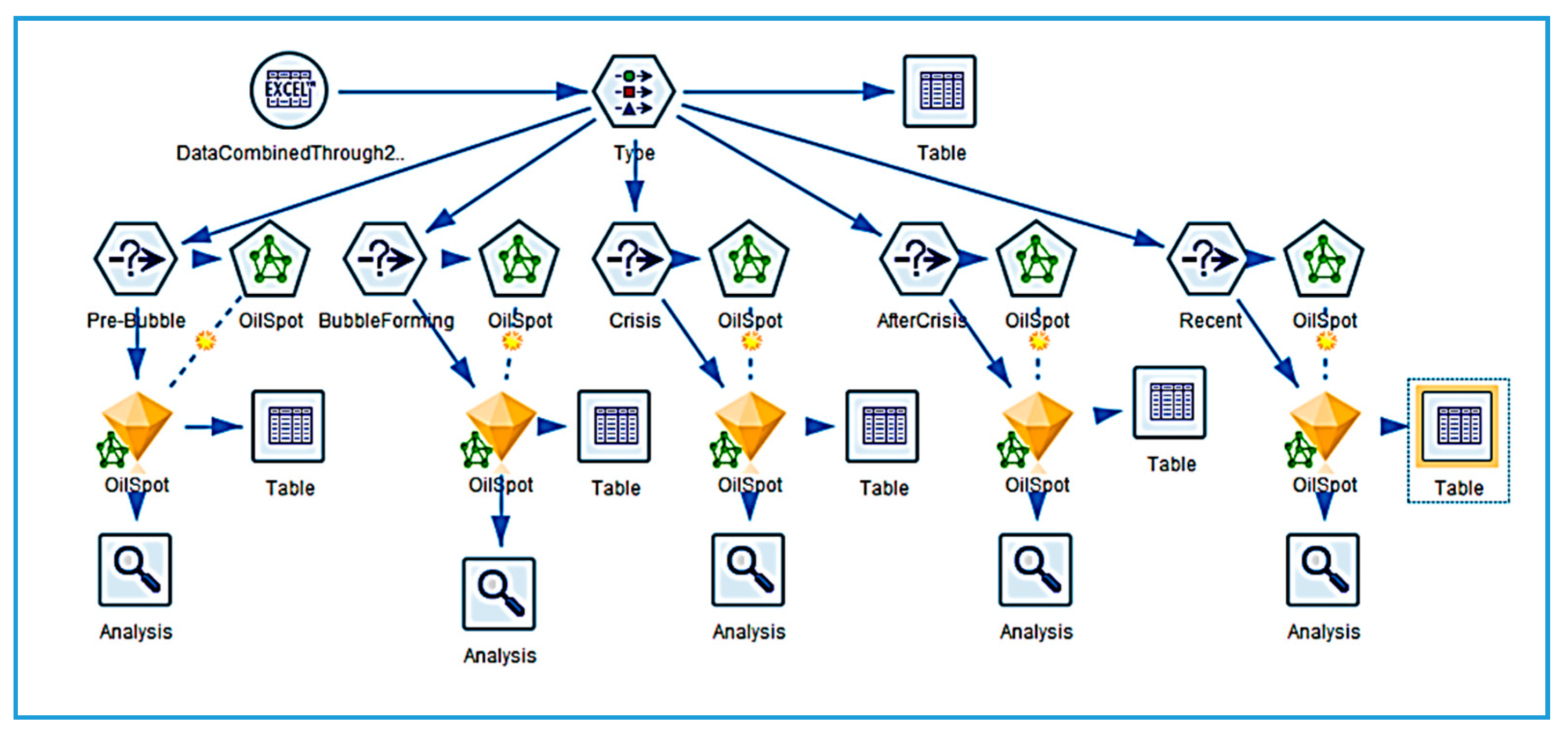
In Modeler, all developments occur through nodes, and they flow from the first node to the last. Nodes are added to the stream by dragging up into the stream the type of node wished for from the possible set at the bottom of the stream’s screen area. Figure 6 illustrates one of the streams constructed for this problem. It shows an Excel node connected to a Type node, then to a Select node followed by a neural network node. The network generates a trained node (shown as a gold nugget) through which it sends data to generate a forecast for each dataset row. The last node, a table, is used to display the results.

Settings within a node are easily accessed by right-clicking on the node and opening a submenu. The data is first read in using an Excel node which forms the connection to the specific data set. It then flows through a Type node where the role each field will play is specified. As Modeler reads the data, it also displays the largest/smallest values the variables take on, the type of data it is assigning to each variable, and whether or not there are any missing or unreadable data in the set. The Type node, opened in its Edit screen, allows all these setting to be checked.

From the Type node, the data are fed through a Select node, which allows the user to narrow the data set to a specific time period. From this node, the data flows to the neural network node. Within the neural network node, the settings for model size and purpose (boosting) are controlled. There are many possible settings within the Edit screen of this node. In Objectives, one can choose to build a standard model, to model for accuracy, or to model for stability. Stopping rule limits can be set for time, for a number of cycles, or for accuracy. When using either boosting or bagging, settings under Ensembles allow the user to specify the type of combining rule that will be used for either continuous or category type targets. Under the Advanced menu, the user can specify the random seed for the network run in order to replicate results, and whether or not missing values will be imputed.

The neural network is then executed and this generates a trained model. The trained model can be browsed to view the sensitivity analysis and structure of the model. Once a trained model is generated, other data sets can be run through it to generate future forecasts or to compare accuracies on a validation set. The trained model’s specific output can be viewed by attaching a table to the trained node and running the data through it. A network similar to the one shown was developed for each of the five data sets.

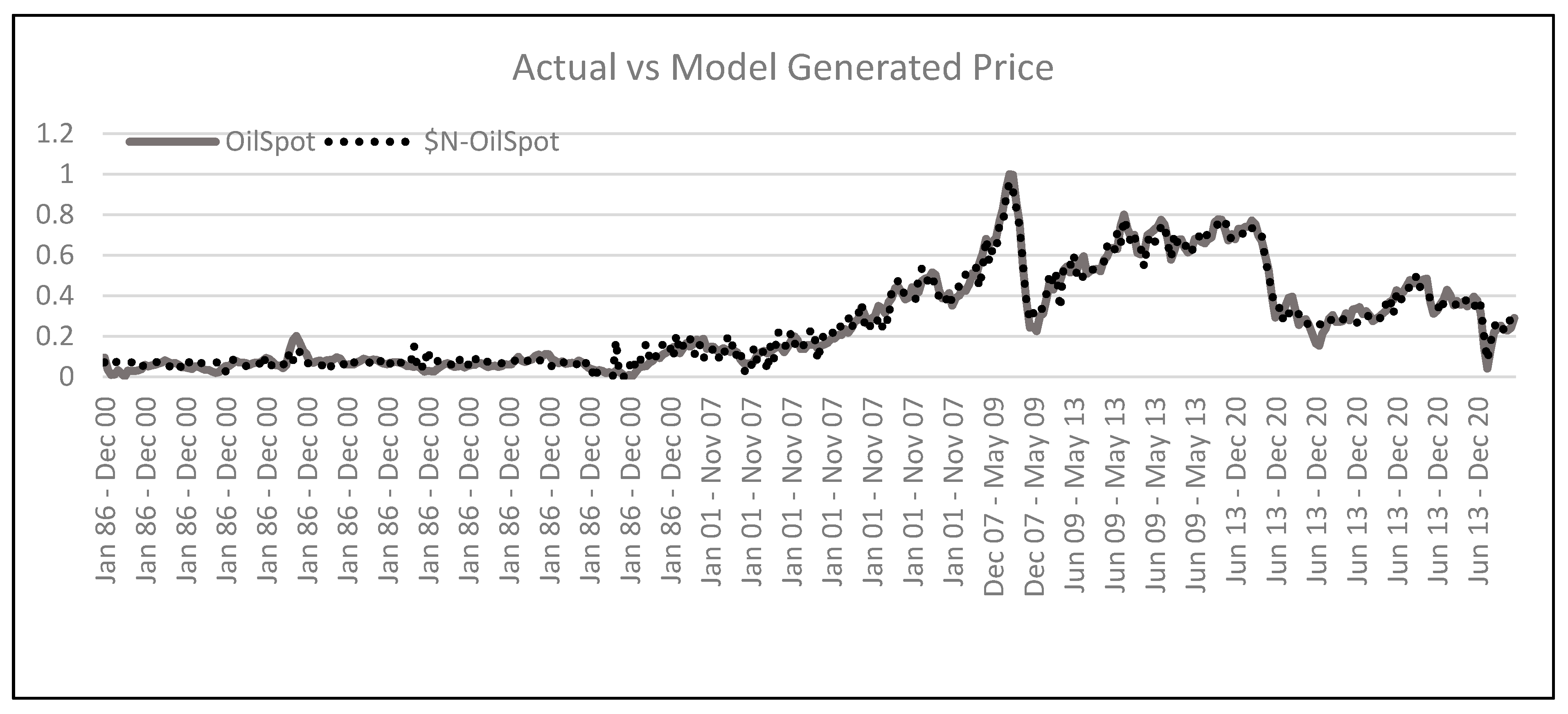
The accuracy of these networks can be seen in the next graph, Figure 7, which shows the actual spot price versus the spot price generated by the trained networks. To generate this graph, the data from all five sets were recombined into a single set. The trained networks closely mimic the actual prices, with a mean absolute deviation of 0.007 across all periods.

With this high level of accuracy, we now turn to the sensitivity analysis. The sensitivity analysis allows us to see the impact of each of the input variables on the neural network target value. The values of a sensitivity analysis are relative to each other and, within a single model, always sum up to one. While these values have no directly interpretable meaning in terms of determining the output value, they do show how the model ranks each input relative to the others in deciding the target’s final value. A larger value indicates a greater impact on the target.

Table 4. Relative importance of variables per data set, largest value in bold.

Input Variable	PreBubble	BubbleForming	Crisis	AfterCrisis	Recent
Consumption	0.16	0.15	0.29	0.07	0.01
Month	0	0	0	0.03	0
NetImports	0.14	0.32	0.21	0.39	0.13
Production	0.21	0.48	0.04	0.23	0.1
StocksExcSPR	0.49	0.05	0.46	0.27	0.76

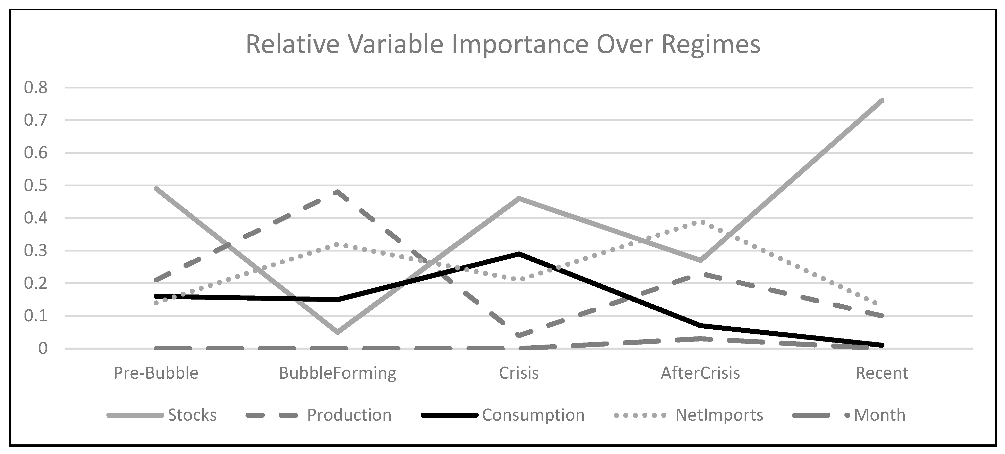
shows the sensitivity analysis (or, relative importance) of each variable on the spot price of oil during each period of time. The variable with the highest impact is highlighted. Figure 8 shows these values in a graph.

The stored stock of oil had the greatest role in determining the spot prices during the pre-bubble, the crisis, and the recent periods. However, in the periods between those, its impact dropped greatly. During the bubble-forming period, production had the greatest impact, and during the period immediately after the crisis, net imports had the most influence on the spot price.

Table 5. Error per period.

	Pre-Bubble	BubbleForming	Crisis	AfterCrisis	Recent
Minimum Error	−0.019	−0.036	−0.016	−0.105	−0.059
Maximum Error	0.024	0.052	0.013	0.019	0.052
Mean Error	0	−0.001	0	−0.003	0.002
Mean Absolute Error	0.004	0.009	0.007	0.008	0.011
Standard Deviation	0.006	0.014	0.008	0.019	0.017
Linear Correlation	0.988	0.996	1	0.978	0.995
Occurrences	180	83	18	48	91

shows the amount of error in the model estimates for each period. A mean absolute error across all periods of 0.007 was recorded. We also see a very high linear correlation between the actual and model-generated values for the target.

4. A Solitary Model

Suppose that, rather than developing individual neural network models for each period, we instead develop one model using all the data. How well would that model do in comparison, and what variables would be the most important? The results from doing this are shown in Figure 9, and in

Table 6. Error calculations for one network for all the data.

Statistic	Value
Minimum Error	−0.152
Maximum Error	0.139
Mean Error	−0.001
Mean Absolute Error	0.031
Standard Deviation	0.04
Linear Correlation	0.985
Occurrences	420

and

Table 7. Relative variable importance over one network.

Variables	Importance
Consumption	0.8772
Month	0.0000036
NetImports	0.0013
Production	0.0294
StocksExcSPR	0.0921

. Figure 9 shows a graph of the two sets of prices over time. The graph shows some periods where the two are close, and some where the prices are more divergent, such as in the late Pre-Bubble and Bubble Forming periods, and at the end of the GFC. Table 6 shows that the overall network spot prices had a mean absolute error from the actual prices of 0.031. This is in comparison to the mean absolute error of 0.007 across the networks developed on individual periods. Table 7 lists the overall variable importance for the inputs. This combined variable importance, generated by one network for all the data, hides from us the changing impact of variables over time. For example, we see in Table 7 that Consumption had a variable importance of 0.8772, much higher than in any individual period. If we were to average the effect of consumption over separate periods, we would get a value of about 0.13. This is about one fourth of the value it has in the single network. StocksExcSPR had the greatest relative importance in three of the five networks on individual sets, but had only an importance of 0.09 here. Inspection of the other inputs shows a similar story of difference in relative importance compared to individually developed networks. By not developing the neural networks for individual regimes, our picture of the variables’ impacts during the separate periods is hidden.

This analysis shows that, by separating the data into regimes motivated by economic reasoning, the neural network results both have a lower error and allow us to see the changing paths of variable influence. We do not claim that the selection of these specific regimes is the optimal set of periods. Further subdivision may give even more insightful results.

5. Conclusions

This paper considers the spot price of oil, net imports of oil, production of oil, the stored supply of oil, and petroleum supplied (a proxy for petroleum consumption) in order to analyze the microeconomic fundamentals of oil in the U.S. markets. Each of these variables was scaled to be between zero and one. In addition, the month of the year was also employed as an input to account for seasonality in the demand for oil. The data were divided into five periods, or regimes, from 1986 through 2020: two before, one during, and two after the GFC of 2007–2009. Using these inputs, we built boosted neural networks to explain the spot price of oil, advancing the hypothesis that different inputs receive fundamental importance along dissimilar economic regimes. Put differently, these networks were built with the intent of analyzing the variables’ impacts across time periods to see whether or not the variable importance remained the same through these very different periods. If we found that a set of variables stayed the same in impact across the financial structural breaks, then we could look for a single network that could be used to successfully forecast across widely varying time periods.

Our methodology shows that, while the inputs into an accurate neural network can remain the same, the impact of each variable changes considerably during different regimes. We find that the shifts in impacts of the various inputs are great enough to support the hypothesis that there are important structural breaks between periods. We conclude that, in the presence of structural breaks, there is a shift in the way the neural network uses and values the inputs. One common approach to forecasting involves a rolling time period for training followed by a short validation set. When structural breaks occur, it is unlikely that this methodology would be successful. A structural break indicates a clear-cut shift in market movement and relationships. Even with frequent re-training, the shift across these breaks is significant enough that the time period for training and that for validation will be so different that the network will not be successful for a future set. With an indication of a structural break, we might need to shift to very short training sets in order to mirror the current relationships.

Our methodological conclusion concurs with Baumeister and Kilian (2016), who conducted a rich and informative narrative of the oil market during the past forty years and concluded that oil prices have continued to surprise us and may continue to do so in the future, both because of the complex fundamentals of this global market and the sequence of unexpected shifts in economic and financial regimes.