


Artificial Neural Network Modeling on PM10, PM2.5, and NO2 Concentrations between Two Megacities without a Lockdown in Korea, for the COVID-19 Pandemic Period of 2020

Abstract
:1. Introduction
2. Materials and Methods
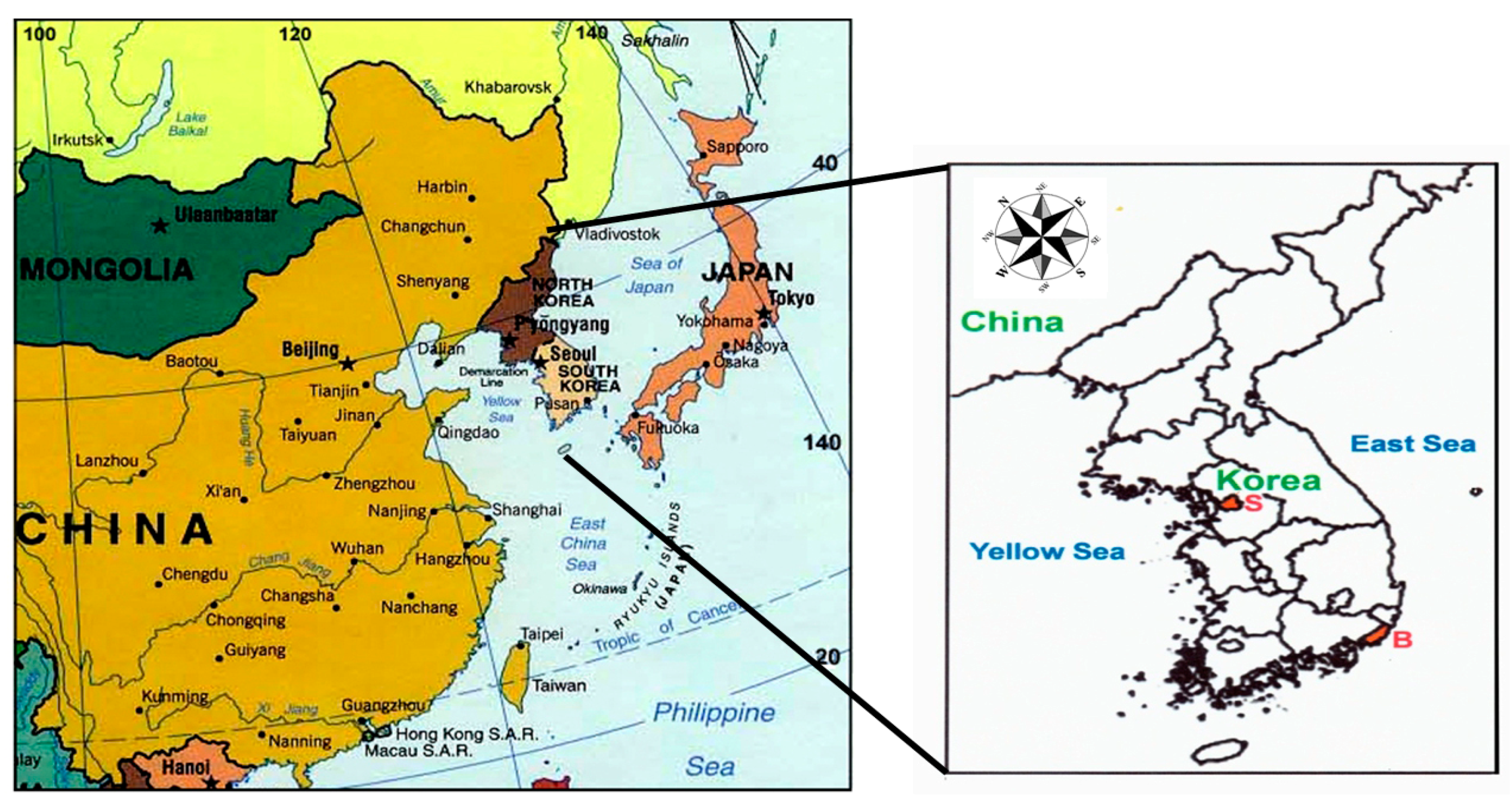
2.1. Study Location

2.2. Air Quality Data Analysis
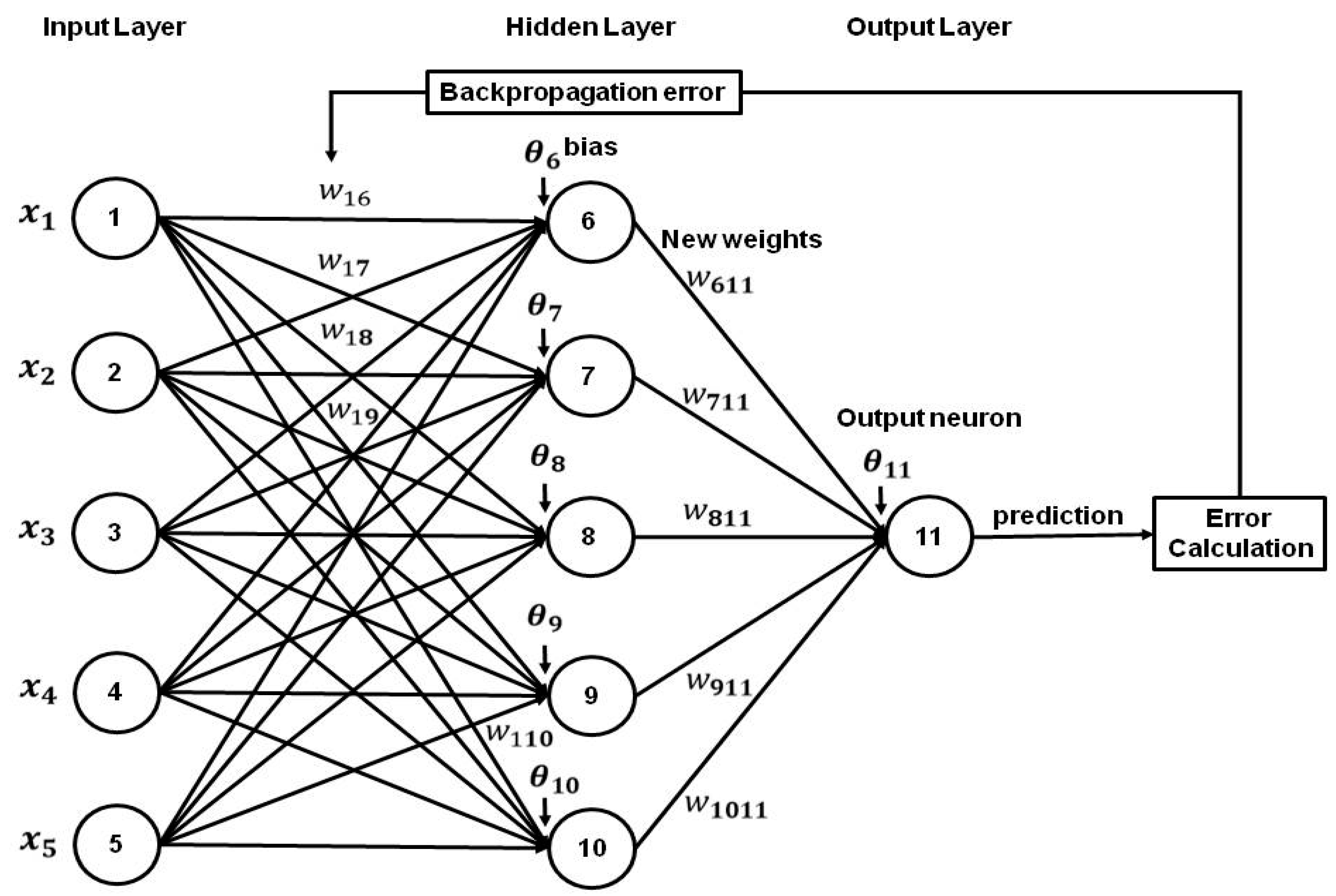
2.3. Artificial Neural Network (ANN)Model—Machine Learning Model

3. Results
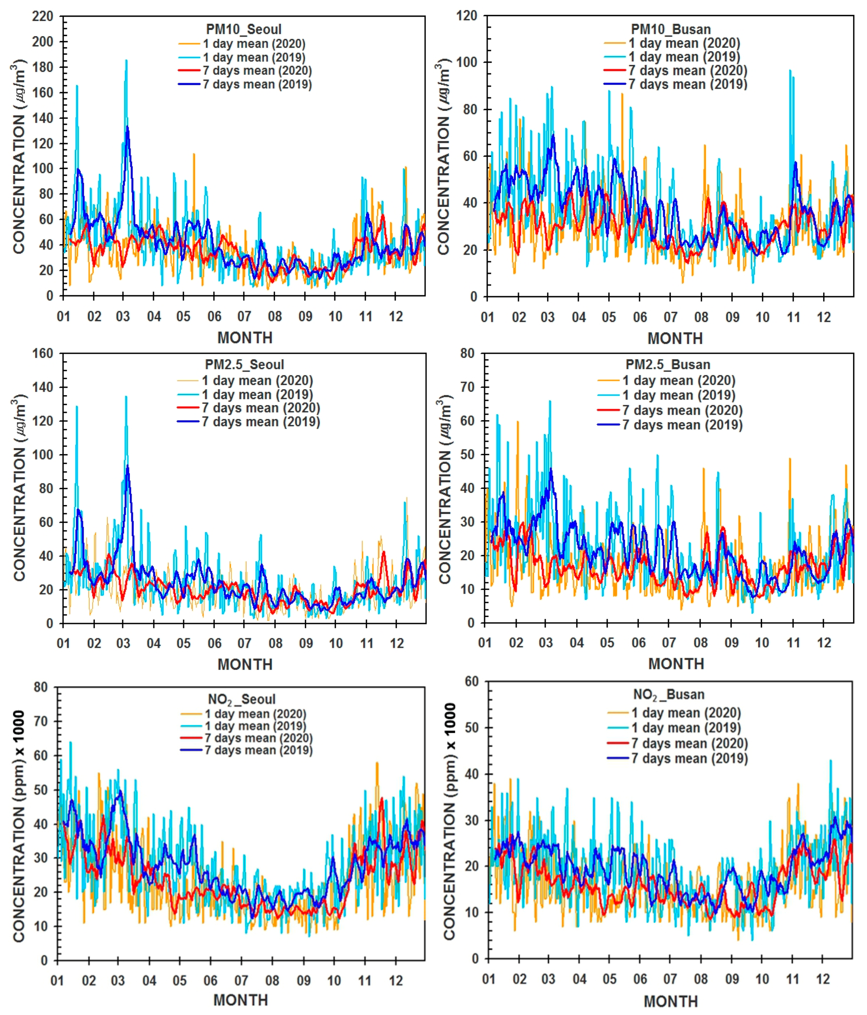
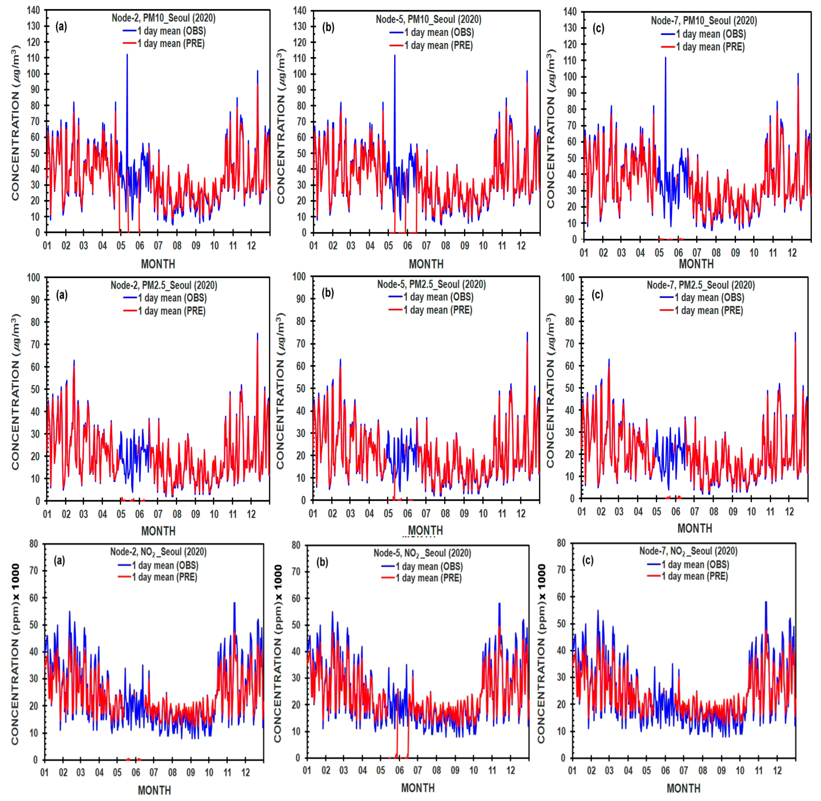
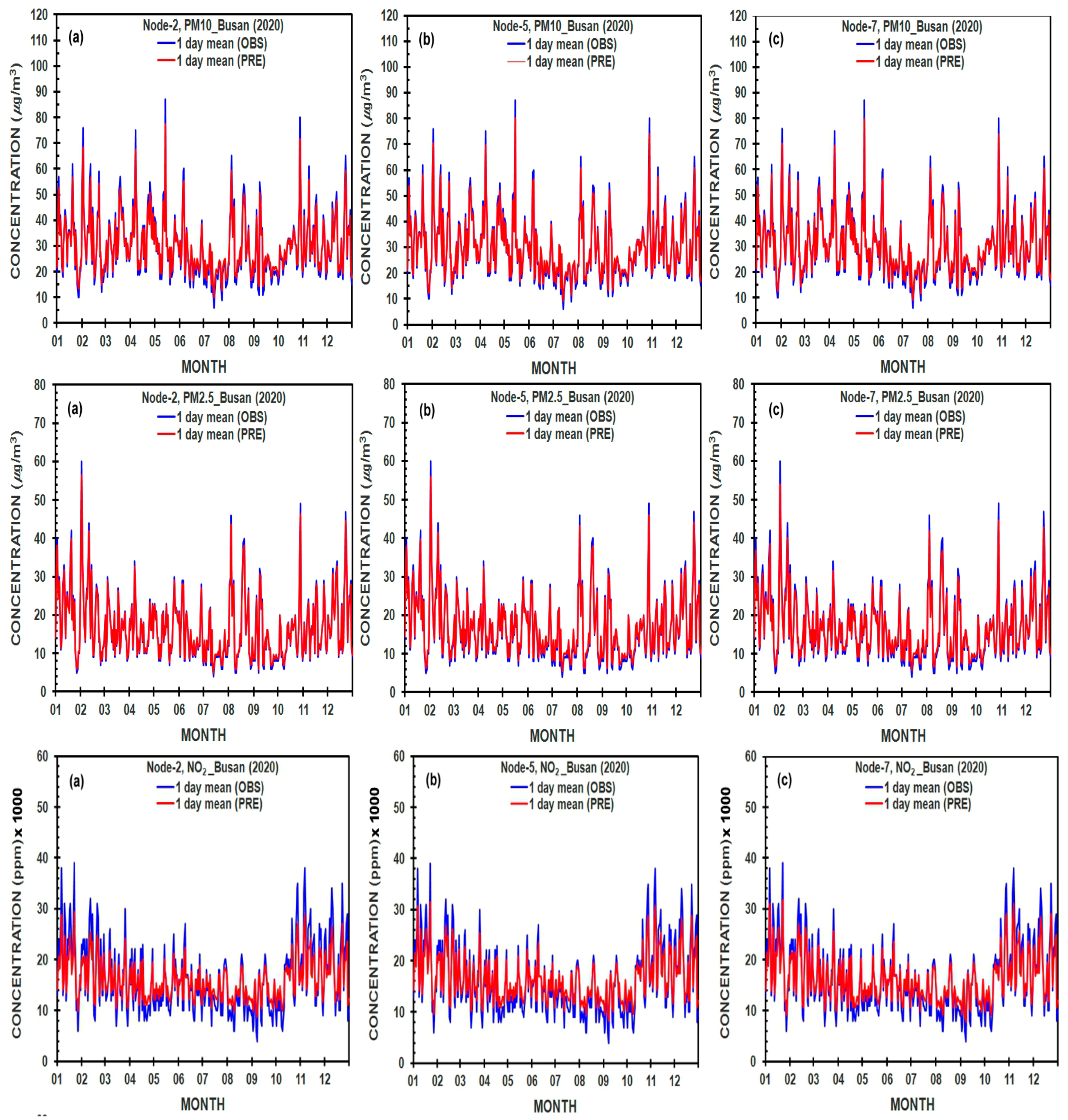
3.1. Temporal Variations of PM10, PM2.5, and NO2 Concentrations at Two Cities

3.2. Evaluation of Daily Mean PM10 and PM2.5, and NO2 Concentrations Using an ANN Model

| Parameter Estimates-PM10(Seoul)-Node=2 | Parameter Estimates-PM10(Busan)-Node=2 | |||||||||
| Hidden Layer 1 | Output Layer | Hidden Layer 1 | Output Layer | |||||||
| Predictor | H(1:1) | H(1:2) | PM10_S | Predictor | H(1:1) | H(1:2) | PM10_B | |||
| Input Layer | (Bias) | −0.297 | −0.051 | Input Layer | (Bias) | 0.458 | 0.230 | |||
| PM2.5_S | 1.201 | −0.871 | PM2.5_B | −1.278 | −1.130 | |||||
| NO2_S | −0.334 | −0.187 | NO2_B | 0.076 | 0.206 | |||||
| PM10_B | 0.337 | −1.408 | PM10_S | −1.154 | −0.949 | |||||
| PM2.5_B | −0.669 | 0.915 | PM2.5_S | 1.423 | 0.512 | |||||
| NO2_B | 0.196 | −0.059 | NO2_S | −0.063 | −0.145 | |||||
| Hidden Layer 1 | (Bias) | 0.189 | Hidden Layer 1 | (Bias) | 2.200 | |||||
| H(1:1) | 2.262 | H(1:1) | −2.381 | |||||||
| H(1:2) | −2.269 | H(1:2) | −1.400 | |||||||
| Parameter Estimates-PM2.5(Seoul)-Node=2 | Parameter Estimates-PM2.5(Busan)-Node=2 | |||||||||
| Hidden Layer 1 | Output Layer | Hidden Layer 1 | Output Layer | |||||||
| Predictor | H(1:1) | H(1:2) | PM2.5_S | Predictor | H(1:1) | H(1:2) | PM2.5_B | |||
| Input Layer | (Bias) | 0.194 | −1.107 | Input Layer | (Bias) | −1.298 | 0.002 | |||
| PM10_S | −1.778 | −0.262 | PM10_B | 0.906 | 3.675 | |||||
| NO2_S | 0.427 | 0.947 | NO2_B | 0.161 | 2.252 | |||||
| PM10_B | 1.142 | 0.298 | PM10_S | −1.083 | 1.542 | |||||
| PM2.5_B | −0.659 | 0.652 | PM2.5_S | 0.986 | 2.774 | |||||
| NO2_B | 0.122 | −0.037 | NO2_S | −0.089 | 1.139 | |||||
| Hidden Layer 1 | (Bias) | 0.925 | Hidden Layer 1 | (Bias) | −1.389 | |||||
| H(1:1) | −2.784 | H(1:1) | 4.984 | |||||||
| H(1:2) | 2.062 | H(1:2) | 0.386 | |||||||
| Parameter Estimates-NO2(Seoul)-Node=2 | Parameter Estimates-NO2(Busan)-Node=2 | |||||||||
| Hidden Layer 1 | Output Layer | Hidden Layer 1 | Output Layer | |||||||
| Predictor | H(1:1) | H(1:2) | NO2_S | Predictor | H(1:1) | H(1:2) | NO2_B | |||
| Input Layer | (Bias) | 0.194 | −0.754 | Input Layer | (Bias) | 0.026 | 1.537 | |||
| PM10_S | −0.850 | 0.039 | PM10_B | 0.056 | −0.118 | |||||
| PM2.5_S | −0.492 | 0.725 | PM2.5_B | −0.840 | −1.292 | |||||
| PM10_B | −0.047 | −0.388 | PM10_S | 0.116 | 0.035 | |||||
| PM2.5_B | −0.082 | −0.222 | PM2.5_S | 0.162 | 0.636 | |||||
| NO2_B | −1.174 | 1.142 | NO2_S | −2.019 | −1.376 | |||||
| Hidden Layer 1 | (Bias) | −0.538 | Hidden Layer 1 | (Bias) | 1.670 | |||||
| H(1:1) | −0.635 | H(1:1) | −0.871 | |||||||
| H(1:2) | 2.501 | H(1:2) | −1.657 | |||||||
| Parameter Estimates-PM10(Seoul)-Node=5 | Parameter Estimates-PM10(Busan)-Node=5 | |||||||||||||||
| Hidden Layer 1 | Output Layer | Hidden Layer 1 | Output Layer | |||||||||||||
| Predictor | H(1:1) | H(1:2) | H(1:3) | H(1:4) | H(1:5) | PM10_S | Predictor | H(1:1) | H(1:2) | H(1:3) | H(1:4) | H(1:5) | PM10_B | |||
| Input Layer | (Bias) | 0.498 | 0.155 | −0.241 | 0.029 | −0.408 | Input Layer | (Bias) | −0.370 | −0.670 | 0.032 | 0.157 | −0.132 | |||
| PM2.5_S | −0.804 | −1.172 | −0.598 | 1.131 | 0.649 | PM2.5_B | −0.895 | 0.827 | 0.681 | −0.812 | 0.937 | |||||
| NO2_S | 0.198 | 0.070 | −0.097 | −0.024 | −0.031 | NO2_B | −0.023 | −0.198 | −0.008 | −0.197 | 0.086 | |||||
| PM10_B | −0.133 | −0.882 | −0.237 | 1.081 | 0.424 | PM10_S | 0.273 | 1.460 | 0.448 | −0.379 | −0.436 | |||||
| PM2.5_B | 0.107 | 0.700 | 0.352 | −1.068 | −0.356 | PM2.5_S | 0.061 | −1.192 | 0.788 | −0.401 | −0.044 | |||||
| NO2_B | 0.086 | 0.318 | −0.392 | 0.246 | 0.135 | NO2_S | 0.026 | 0.212 | 0.441 | 0.099 | −0.406 | |||||
| Hidden Layer 1 | (Bias) | 0.134 | Hidden Layer 1 | (Bias) | −1.184 | |||||||||||
| H(1:1) | −0.485 | H(1:1) | −0.766 | |||||||||||||
| H(1:2) | −1.284 | H(1:2) | 3.524 | |||||||||||||
| H(1:3) | −0.522 | H(1:3) | −0.108 | |||||||||||||
| H(1:4) | 1.585 | H(1:4) | −0.296 | |||||||||||||
| H(1:5) | 0.789 | H(1:5) | 1.009 | |||||||||||||
| Parameter Estimates-PM2.5(Seoul)-Node=5 | Parameter Estimates-PM2.5(Busan)-Node=5 | |||||||||||||||
| Hidden Layer 1 | Output Layer | Hidden Layer 1 | Output Layer | |||||||||||||
| Predictor | H(1:1) | H(1:2) | H(1:3) | H(1:4) | H(1:5) | PM2.5_S | Predictor | H(1:1) | H(1:2) | H(1:3) | H(1:4) | H(1:5) | PM2.5_B | |||
| Input Layer | (Bias) | −0.075 | −0.861 | 1.332 | −0.173 | −0.923 | Input Layer | (Bias) | 0.145 | −0.104 | −0.383 | −1.881 | −0.312 | |||
| PM10_S | −0.312 | 0.518 | −0.238 | 1.866 | 1.008 | PM10_B | 1.510 | 0.240 | −0.865 | 0.742 | −0.021 | |||||
| NO2_S | 1.090 | 0.103 | −0.708 | −1.181 | 0.012 | NO2_B | 0.220 | 0.246 | −0.199 | 0.288 | −0.019 | |||||
| PM10_B | 0.140 | −1.284 | 0.430 | −0.397 | −0.576 | PM10_S | 0.095 | −0.237 | 0.360 | −1.573 | 0.261 | |||||
| PM2.5_B | 0.607 | 0.880 | −0.729 | 0.009 | 0.511 | PM2.5_S | −0.176 | 0.857 | −0.228 | 1.482 | 0.279 | |||||
| NO2_B | −0.039 | 0.156 | 0.398 | 0.032 | −0.136 | NO2_S | −0.040 | 0.120 | −0.244 | −0.527 | −0.268 | |||||
| Hidden Layer 1 | (Bias) | −0.892 | Hidden Layer 1 | (Bias) | −1.361 | |||||||||||
| H(1:1) | 1.202 | H(1:1) | 1.175 | |||||||||||||
| H(1:2) | 1.277 | H(1:2) | 1.066 | |||||||||||||
| H(1:3) | −1.468 | H(1:3) | −0.756 | |||||||||||||
| H(1:4) | 1.652 | H(1:4) | 3.134 | |||||||||||||
| H(1:5) | 0.936 | H(1:5) | 0.256 | |||||||||||||
| Parameter Estimates-NO2(Seoul)-Node=5 | Parameter Estimates-NO2(Busan)-Node=5 | |||||||||||||||
| Hidden Layer 1 | Output Layer | Hidden Layer 1 | Output Layer | |||||||||||||
| Predictor | H(1:1) | H(1:2) | H(1:3) | H(1:4) | H(1:5) | NO2_S | Predictor | H(1:1) | H(1:2) | H(1:3) | H(1:4) | H(1:5) | NO2_B | |||
| Input Layer | (Bias) | 0.134 | −0.003 | −0.774 | −0.273 | 0.069 | Input Layer | (Bias) | −0.186 | −0.031 | 0.003 | −0.432 | −0.181 | |||
| PM10_S | −0.392 | −0.450 | −0.133 | −0.536 | −0.224 | PM10_B | 0.281 | −0.002 | −0.158 | 0.032 | 0.274 | |||||
| PM2.5_S | −0.307 | 0.465 | 0.804 | 0.043 | −0.484 | PM2.5_B | −0.660 | 0.574 | 0.410 | 0.751 | −0.366 | |||||
| PM10_B | 0.152 | 0.234 | 0.207 | 0.493 | −0.281 | PM10_S | −0.531 | 0.080 | 0.069 | −0.088 | 0.518 | |||||
| PM2.5_B | 0.347 | −0.574 | −0.377 | −0.242 | 0.508 | PM2.5_S | −0.668 | 0.464 | −0.084 | −0.478 | 0.011 | |||||
| NO2_B | −0.743 | 0.957 | 0.859 | −0.502 | −0.314 | NO2_S | −0.317 | 1.006 | 0.797 | 1.010 | 0.231 | |||||
| Hidden Layer 1 | (Bias) | −0.075 | Hidden Layer 1 | (Bias) | −1.357 | |||||||||||
| H(1:1) | −0.973 | H(1:1) | −0.199 | |||||||||||||
| H(1:2) | 1.219 | H(1:2) | 0.590 | |||||||||||||
| H(1:3) | 1.319 | H(1:3) | 0.872 | |||||||||||||
| H(1:4) | −0.406 | H(1:4) | 1.816 | |||||||||||||
| H(1:5) | −0.558 | H(1:5) | 0.091 | |||||||||||||
| Parameter Estimates-PM10(Seoul)-Node=7 | Output Layer | Parameter Estimates-PM10(Busan)-Node=7 | Output Layer | |||||||||||||||||
| Hidden Layer 1 | Hidden Layer 1 | |||||||||||||||||||
| Predictor | H(1:1) | H(1:2) | H(1:3) | H(1:4) | H(1:5) | H(1:6) | H(1:7) | PM10_S | Predictor | H(1:1) | H(1:2) | H(1:3) | H(1:4) | H(1:5) | H(1:6) | H(1:7) | PM10_B | |||
| Input Layer | (Bias) | 0.477 | 0.337 | −0.379 | −0.192 | −0.023 | −0.369 | 0.068 | Input Layer | (Bias) | 1.069 | −0.770 | −0.648 | 0.176 | 0.307 | −0.285 | −1.063 | |||
| PM2.5_S | −0.046 | 0.445 | −0.709 | −0.958 | 1.011 | 0.947 | −1.066 | PM2.5_B | −0.972 | 0.561 | 0.957 | −0.128 | 0.522 | −0.550 | 0.861 | |||||
| NO2_S | −0.264 | −0.220 | 0.151 | −0.328 | −0.277 | 0.075 | −0.155 | NO2_B | 0.023 | −0.111 | 0.020 | −0.115 | −0.241 | −0.009 | −0.008 | |||||
| PM10_B | −0.422 | 0.248 | −0.184 | −0.387 | 0.122 | 0.880 | −0.155 | PM10_S | −0.370 | 1.310 | 0.198 | −0.987 | −0.167 | −0.603 | 0.964 | |||||
| PM2.5_B | −0.085 | −0.341 | 0.323 | 0.263 | −0.149 | −0.751 | −0.087 | PM2.5_S | 1.345 | −0.739 | −0.304 | 0.105 | −0.296 | 0.343 | −0.919 | |||||
| NO2_B | 0.444 | −0.347 | −0.050 | −0.125 | 0.167 | −0.102 | −0.219 | NO2_S | −0.204 | −0.276 | 0.152 | −0.029 | 0.344 | 0.549 | 0.219 | |||||
| Hidden Layer 1 | (Bias) | 0.200 | Hidden Layer 1 | (Bias) | −0.158 | |||||||||||||||
| H(1:1) | −0.355 | H(1:1) | −1.248 | |||||||||||||||||
| H(1:2) | 0.561 | H(1:2) | 1.351 | |||||||||||||||||
| H(1:3) | −0.710 | H(1:3) | 0.800 | |||||||||||||||||
| H(1:4) | −0.909 | H(1:4) | −0.460 | |||||||||||||||||
| H(1:5) | 0.625 | H(1:5) | 0.606 | |||||||||||||||||
| H(1:6) | 1.277 | H(1:6) | −0.433 | |||||||||||||||||
| H(1:7) | −0.798 | H(1:7) | 1.379 | |||||||||||||||||
| Parameter Estimates-PM2.5(Seoul)-Node=7 | Output Layer | Parameter Estimates-PM2.5(Busan)-Node=7 | Output Layer | |||||||||||||||||
| Hidden Layer 1 | Hidden Layer 1 | |||||||||||||||||||
| Predictor | H(1:1) | H(1:2) | H(1:3) | H(1:4) | H(1:5) | H(1:6) | H(1:7) | PM2.5_S | Predictor | H(1:1) | H(1:2) | H(1:3) | H(1:4) | H(1:5) | H(1:6) | H(1:7) | PM2.5_B | |||
| Input Layer | (Bias) | 0.363 | −0.119 | −0.245 | 0.004 | −0.176 | −0.594 | −0.213 | Input Layer | (Bias) | −0.212 | 0.242 | −0.543 | −0.006 | −0.447 | −0.372 | 0.151 | |||
| PM10_S | −0.919 | 0.202 | −0.149 | −1.127 | −0.030 | 0.578 | 0.202 | PM10_B | 0.147 | −1.131 | 1.127 | −0.403 | 0.133 | 0.141 | 0.584 | |||||
| NO2_S | −0.020 | 0.175 | −0.341 | 0.245 | −0.087 | 0.495 | 0.084 | NO2_B | 0.347 | −0.176 | 0.275 | −0.072 | 0.207 | 0.652 | 0.283 | |||||
| PM10_B | 0.139 | −0.450 | 0.397 | 0.272 | −1.009 | −0.614 | −0.644 | PM10_S | −0.032 | 0.657 | −1.120 | 0.207 | −0.099 | 0.135 | −0.763 | |||||
| PM2.5_B | −0.637 | 0.265 | −0.440 | −0.235 | 0.005 | 0.800 | 0.627 | PM2.5_S | −0.706 | −0.358 | 1.134 | −0.551 | 0.479 | 0.163 | 0.418 | |||||
| NO2_B | 0.170 | 0.101 | −0.290 | 0.052 | −0.710 | −0.276 | 0.412 | NO2_S | −0.005 | −0.116 | −0.717 | −0.225 | −0.110 | −0.115 | 0.423 | |||||
| Hidden Layer 1 | (Bias) | 0.636 | Hidden Layer 1 | (Bias) | −0.299 | |||||||||||||||
| H(1:1) | −1.669 | H(1:1) | −0.587 | |||||||||||||||||
| H(1:2) | 0.361 | H(1:2) | −1.098 | |||||||||||||||||
| H(1:3) | −0.812 | H(1:3) | 1.861 | |||||||||||||||||
| H(1:4) | −1.468 | H(1:4) | −0.545 | |||||||||||||||||
| H(1:5) | 0.876 | H(1:5) | 0.448 | |||||||||||||||||
| H(1:6) | 1.242 | H(1:6) | 0.242 | |||||||||||||||||
| H(1:7) | 0.859 | H(1:7) | 0.892 | |||||||||||||||||
| Parameter Estimates-NO2(Seoul)-Node=7 | Output Layer | Parameter Estimates-NO2(Busan)-Node=7 | Output Layer | |||||||||||||||||
| Hidden Layer 1 | Hidden Layer 1 | |||||||||||||||||||
| Predictor | H(1:1) | H(1:2) | H(1:3) | H(1:4) | H(1:5) | H(1:6) | H(1:7) | NO2_S | Predictor | H(1:1) | H(1:2) | H(1:3) | H(1:4) | H(1:5) | H(1:6) | H(1:7) | NO2_B | |||
| Input Layer | (Bias) | −0.442 | 0.873 | −0.430 | 0.055 | −0.550 | 0.693 | 0.240 | Input Layer | (Bias) | −0.265 | −0.560 | −0.074 | 0.053 | −0.428 | 0.474 | −0.474 | |||
| PM10_S | 0.083 | −0.136 | −0.650 | 0.167 | 0.652 | 0.205 | −0.238 | PM10_B | −0.024 | −0.357 | 0.178 | 0.927 | −0.392 | −0.156 | 0.044 | |||||
| PM2.5_S | 0.287 | −1.147 | 0.671 | −0.039 | 0.391 | −0.393 | 0.371 | PM2.5_B | −0.419 | 0.588 | 0.305 | 0.454 | −0.533 | 0.450 | 0.464 | |||||
| PM10_B | −0.234 | 0.469 | 0.448 | −0.118 | 0.161 | −0.231 | 0.085 | PM10_S | −0.152 | −0.148 | −0.156 | 0.793 | −0.731 | 0.053 | 0.453 | |||||
| PM2.5_B | 0.114 | 0.233 | 0.221 | −0.090 | −0.638 | 0.341 | −0.864 | PM2.5_S | −0.729 | −0.389 | 0.337 | 0.718 | −0.859 | −0.049 | −0.604 | |||||
| NO2_B | −0.180 | −1.042 | 0.321 | −0.272 | 0.851 | −0.629 | 0.728 | NO2_S | −0.943 | 0.647 | −0.037 | 1.443 | −1.103 | 0.433 | 1.082 | |||||
| Hidden Layer 1 | (Bias) | 0.164 | Hidden Layer 1 | (Bias) | −0.197 | |||||||||||||||
| H(1:1) | −0.045 | H(1:1) | −0.497 | |||||||||||||||||
| H(1:2) | −1.189 | H(1:2) | 1.292 | |||||||||||||||||
| H(1:3) | 0.638 | H(1:3) | −0.207 | |||||||||||||||||
| H(1:4) | −0.130 | H(1:4) | −1.121 | |||||||||||||||||
| H(1:5) | 0.921 | H(1:5) | −1.084 | |||||||||||||||||
| H(1:6) | −0.697 | H(1:6) | 0.249 | |||||||||||||||||
| H(1:7) | 1.009 | H(1:7) | 2.409 | |||||||||||||||||
3.3. Statistical Performance of the Optimal ANN Model with Data Sets of Training, Testing, and Validation
| Variables | Hidden Neuron Numbers | RMSE | R2 | ||||
|---|---|---|---|---|---|---|---|
| Training | Testing | Validation | Training | Testing | Validation | ||
| PM10-Seoul | 2 | 2.438 | 2.251 | 2.251 | 0.864 | 0.894 | 0.882 |
| 5 | 2.959 | 1.745 | 1.909 | 0.868 | 0.870 | 0.896 | |
| 7 | 1.904 | 1.738 | 1.913 | 0.892 | 0.884 | 0.892 | |
| PM2.5-Seoul | 2 | 1.076 | 1.511 | 0.717 | 0.921 | 0.900 | 0.925 |
| 5 | 0.836 | 1.193 | 0.955 | 0.932 | 0.904 | 0.930 | |
| 7 | 0.847 | 1.196 | 0.955 | 0.938 | 0.905 | 0.922 | |
| NO2-Seoul | 2 | 3.369 | 3.305 | 3.502 | 0.704 | 0.699 | 0.729 |
| 5 | 3.256 | 4.024 | 2808 | 0.720 | 0.685 | 0.746 | |
| 7 | 3.032 | 3.456 | 3.481 | 0.722 | 0.722 | 0.734 | |
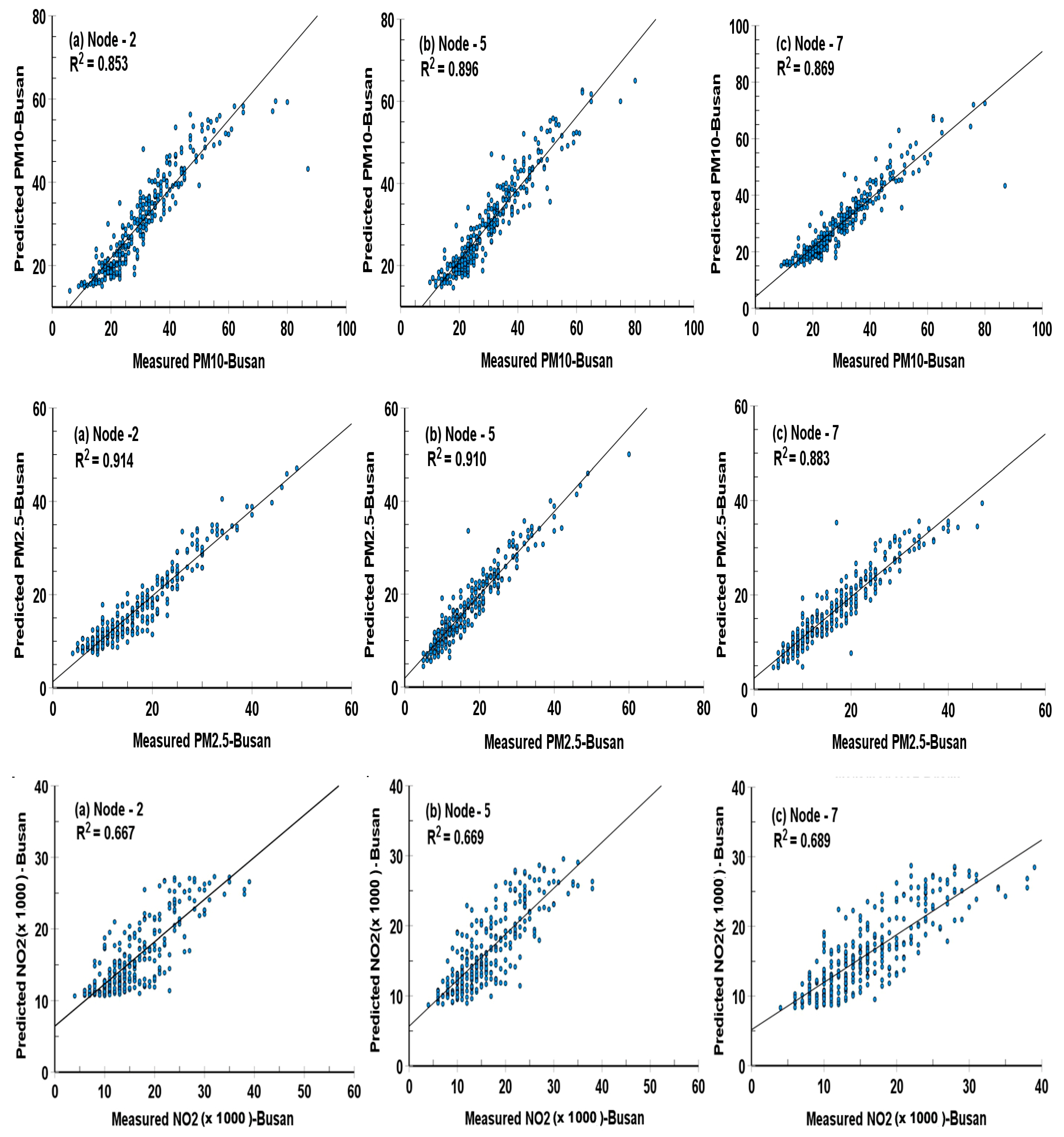
| PM10-Busan | 2 | 1.772 | 1.774 | 2.155 | 0.855 | 0.864 | 0.853 |
| 5 | 1.392 | 2.155 | 1.519 | 0.896 | 0.866 | 0.896 | |
| 7 | 1.392 | 1.645 | 1.649 | 0.901 | 0.878 | 0.869 | |
| PM2.5-Busan | 2 | 0.951 | 1.056 | 0.692 | 0.896 | 0.894 | 0.914 |
| 5 | 0.609 | 1.995 | 0.891 | 0.934 | 0.850 | 0.910 | |
| 7 | 0.607 | 1.127 | 1.211 | 0.940 | 0.878 | 0.883 | |
| NO2-Busan | 2 | 2.606 | 2.740 | 2.747 | 0.617 | 0.621 | 0.667 |
| 5 | 2.205 | 2.594 | 2.277 | 0.667 | 0.623 | 0.669 | |
| 7 | 2.140 | 2.284 | 2.137 | 0.680 | 0.663 | 0.689 | |
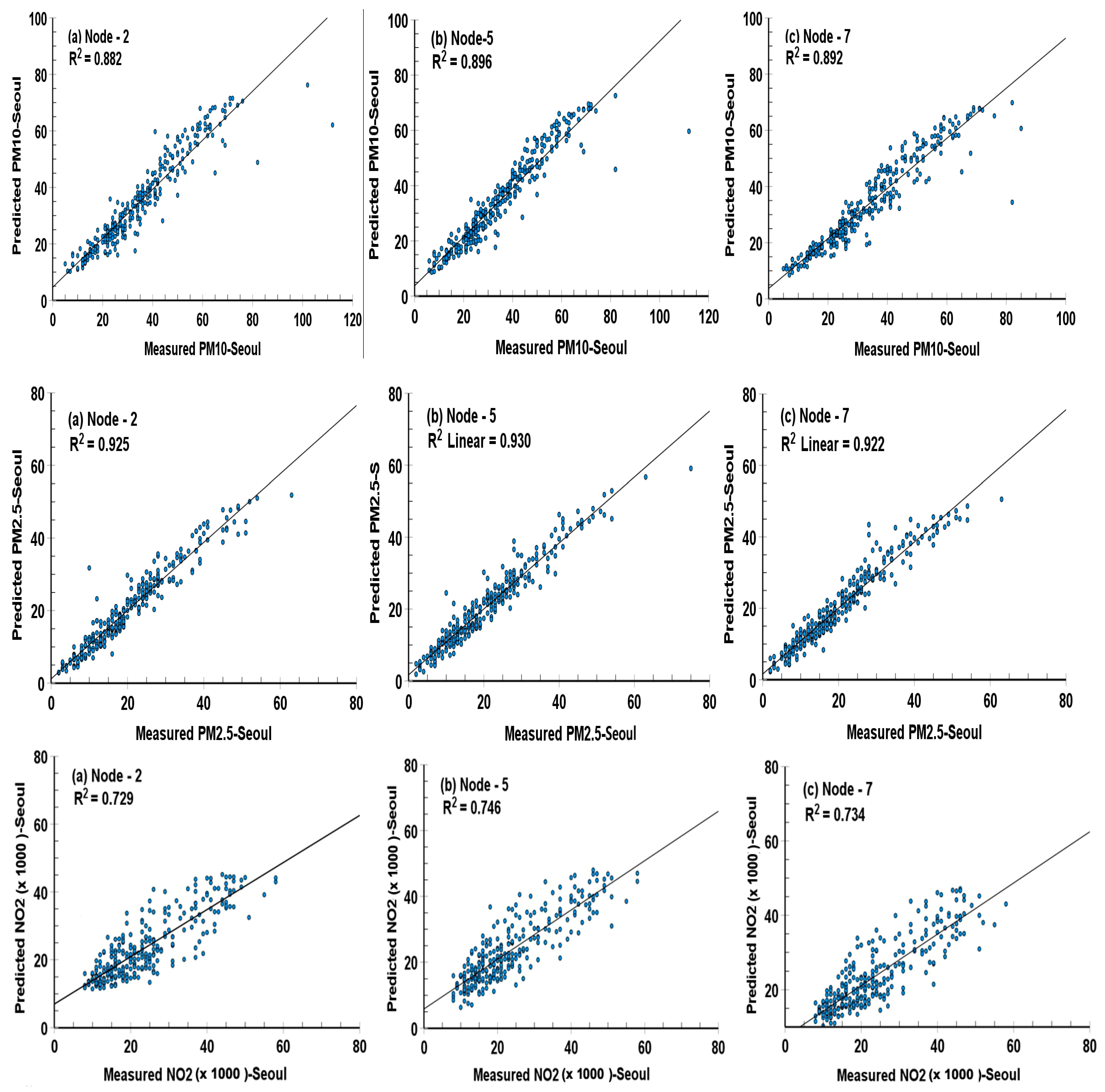
3.4. Scatter Plots for the Performance of an Optimal ANN Model with Different Numbers of Nodes in a Hidden Layer


3.5. Sensitivity of the Performance of an Optimal ANN Model with Different Numbers of Nodes in a Hidden Layer

4. Conclusions
Author Contributions
Funding
Data Availability Statement
Acknowledgments
Conflicts of Interest
References
- NHC (National Health Commission of the People’s Republic of China, Beijing, China). Diagnosis and Treatment Guideline on Pneumonia Infection with 2019 Novel Coronavirus, 5th, ed.; NHC: Beijing, China, 2020.
- Han, Y.; Lam, J.C.K.; Li, V.O.K.; Guo, P.; Zhang, Q.; Wang, A.; Crowcroft, J.; Wang, S.; Fu, J.; Gilani, Z. The effects of outdoor air pollution concentrations and lockdowns on COVID-19 infections in Wuhan and other provincial capitals in China. Preprints 2020, 2020030364. [Google Scholar] [CrossRef] [Green Version]
- WHO (World Health Organization). Coronavirus Disease 2019 (COVID-19) Situation Report, 2020, 51. Available online: https://www.who.int/emergenices/diseases/novel-coronavirus-2019/situationreports (accessed on 10 January 2021).
- Ming, W.; Zhou, Z.; Ai, H.; Bi, H.; Zhong, Y. COVID-19 and air quality: Evidence from China. Emerg. Mark. Financ. Trade 2020, 56, 2422–2442. [Google Scholar] [CrossRef]
- Liu, S.; Kong, G.; Kong, D. Effects of the COVID-19 on air quality: Human mobility, spillover effects, and city connections. Environ. Resour. Econ. 2020, 76, 635–653. [Google Scholar] [CrossRef]
- Brimblecombe, P.; Lai, Y. Effect of sub-urban scale lockdown on air pollution in Beijing. Urban Clim. 2020, 34, 100725. [Google Scholar] [CrossRef]
- Pei, Z.; Han, G.; Ma, X.; Su, H.; Gong, W. Response of major air pollutants to COVID-19 lockdown in China. Sci. Total Environ. 2020, 743, 140879. [Google Scholar] [CrossRef] [PubMed]
- Feng, S.; Jiang, F.; Wang, H.; Ju, W.; Shen, Y.; Zheng, Y.; Wu, Z.; Ding, A. NOx emission changes over China during the COVID-19 epidemic inferred from surface NO2 observations. Geophys. Res. Lett. 2020, 47, e2020GL090080. [Google Scholar] [CrossRef]
- Bao, R.; Zhang, A. Does lockdown reduce air pollution? Evidence from 44 cities in northern China. Sci. Total Environ. 2020, 731, 139052. [Google Scholar] [CrossRef]
- Yuan, Q.; Qi, B.; Hu, D.; Wang, J.; Zhang, J.; Yang, H.; Zhang, S.; Liu, L.; Xu, L.; Li, W. Spatiotemporal variations and reduction of air pollutants during the COVID-19 pandemic in a megacity of Yangze river delta in China. Sci. Total Environ. 2020, 751, 141820. [Google Scholar] [CrossRef]
- Yao, Y.; Pan, J.; Liu, Z.; Meng, X.; Wang, W.; Kan, H. Ambient nitrogen dioxide and spreadability of COVID-19 in Chinese cities. Ecotox. Environ. Saf. 2021, 208, 111421. [Google Scholar] [CrossRef]
- Zhang, R.; Zhang, Y.; Lin, H.; Feng, X.; Fu, T.M.; Wang, Y. NOx emission reduction and recovery during COVID-19 in east China. Atmosphere 2020, 11, 433. [Google Scholar] [CrossRef]
- Chu, B.; Zhang, S.; Liu, J.; Ma, Q.; He, H. Significant concurrent decrease in PM2.5 and NO2 concentrations in China during COVID-19 epidemic. J. Env. Sci. 2021, 99, 346–353. [Google Scholar] [CrossRef] [PubMed]
- Dhaka, S.K.; Chetna; Kumar, V.; Dimri, V.P.; Singh, N.; Patra, K.; Matsumi, Y.; Takigawa, M.; Nakayama, T.; Yamaji, K.; et al. PM2.5 diminution and haze events over Delhi during the COVID-19 lockdown period: An inetrplay between the baseline pollution and meteorology. Sci. Rep. 2020, 10, 13442. [Google Scholar] [CrossRef] [PubMed]
- Kumar, P.; Hama, S.; Omidvarboma, H.; Sharma, A.; Sahani, J.; Abhijith, K.V. Temporary reduction in fine particulate matter due to anthropogenic emissions switch-off during COVID-19 lockdown in Indian cities. Sutain. Cities Soc. 2020, 62, 102382. [Google Scholar] [CrossRef] [PubMed]
- Datta, A.S.; Sahu, A.S. Spatio-temporal analysis of improvement in air quality following corona virus pandemic induced lockdown and suspension of vehicular movement: A case study in Kolkata metropolitan core and its adjacent area. Inter. J. Eng. Manag. Human. 2021, 1, 48–67. [Google Scholar]
- Bherwani, H.; Gautan, S.; Gupta, A. Qualitative and quantitative analysis of impact of COVID-19 on sustainable development goals(SDGs) in Indian subcontinent with a focus on air quality. Inter. J. Environ. Sci. Technol. 2021, 18, 1019–1028. [Google Scholar] [CrossRef] [PubMed]
- Coker, E.S.; Cavalli, L.; Fabrizi, E.; Guastella, G.; Lippo, E.; Parisi, M.L.; Pontarollo, N.; Rizzati, M.; Varacca, A.; Vergalli, S. The effects of air pollution on COVID-19 related mortality in Northern Italy. Environ. Resour. Econ. 2020, 76, 611–634. [Google Scholar] [CrossRef]
- Zoran, M.; Savastru, R.; Savastru, D.; Tautan, M.N. Assessing the relationship between surface levels of PM2.5 and PM10 particulate matter impaction COVID-19 in Milan, Italy. Sci. Total Environ. 2020, 738, 139825. [Google Scholar] [CrossRef]
- Akvile, F.S.; Zaneta, S. COVID-19 and air pollution: Measuring pandemic impact to air quality in five European countries. Atmosphere 2021, 12, 290. [Google Scholar]
- Tobias, A.; Carnerero, C.; Reche, C.; Massague, J.; Via, M.; Minguillon, M.C. Changes in air quality during the lockdown in Barcelona(Spain) one month into the SARS-CoV-2 epidemic. Sci. Total Environ. 2020, 726, 138540. [Google Scholar] [CrossRef]
- Magazzino, C.; Mele, M.; Sarkodie, S.A. The nexus between COVID-19 deaths, air pollution and economic growth in New York state: Evidence from Deep Machine Learning. J. Environ. Manag. 2021, 286, 112241. [Google Scholar] [CrossRef]
- Wang, T.; Nie, W.; Gao, J.; Xue, L.K.; Gao, X.M.; Wang, X.F. Air quality during the 2008 Beijing Olympics: Secondary pollutants and regional impact. Atmos. Chem. Phys. 2010, 10, 7603–7615. [Google Scholar] [CrossRef] [Green Version]
- Xing, J.; Zhang, Y.; Wang, S.; Liu, X.; Cheng, S.; Zhang, Q. Modeling study on the air quality impacts from emission reductions and typical meteorological conditions during the 2008 Beijing Olympics. Atmos. Environ. 2011, 45, 1786–1798. [Google Scholar] [CrossRef]
- Sun, Y.L.; Wang, Z.F.; Wild, O.; Xu, W.Q.; Chen, C.; Fu, P.Q. “APEC blue”: Secondary aerosol reductions from emission controls in Beijing. Sci. Rep. 2016, 6, 20668. [Google Scholar] [CrossRef] [PubMed] [Green Version]
- Xu, W.; Liu, X.J.; Liu, L.; Dore, A.O.; Tang, A.H.; Lu, L. Impact of emission controls on air quality in Beijing during APEC 2014: Implications from water-soluble ions and carbonaceous aerosol in PM2.5 and their precursors. Atmos. Environ. 2019, 210, 241–252. [Google Scholar] [CrossRef]
- Lei, M.T.; Monjardino, J.; Mendes, L.; Goncalves, D.; Ferreira, F. Statistical forecast of pollution episodes in Macao during National Holiday and COVID-19. Int. J. Env. Res. Pub. Health 2020, 17, 5124. [Google Scholar] [CrossRef]
- Hong, K.; Yum, S.; Kim, J.; Chun, B.C. The serial interval of COVID-19 in Korea; 1567 pairs of symptomatic cases from contact tracing. J. Korea Med. Sci. 2020, 35, 50, e435-1–e435-5. [Google Scholar] [CrossRef]
- Choi, J.; Lee, H.; Park, J.; Cho, S.; Kwon, M.; Jo, C.; Koh, Y.H. Altered COVID-19 receptor ACE2 expression in a higher risk group for cerebrovascular disease and ischemic stroke. Biochem. Biophys. Res. Commun. 2020, 528, 413–419. [Google Scholar] [CrossRef]
- Real Time Report on COVID-19 Epidemic; KDCPA (the Korea Disease Control and Prevention Agency): Cheongju-si, Republic of Korea, 2020.
- Park, D.; Kim, H.Y.; Jo, S.K.; Lee, H.J.; Park, J.S.; Lee, N.J.; Woo, S.H.; Kim, J.M.; Kim, G.J. Effect of virus variants on COVID-19 diagnosis in the Republic of Korea. Pub. Health Week. Rep. 2021, 14, 3236–3238. [Google Scholar]
- KEC (Korea Environment Corporation). Available online: https://www.airkorea.or.kr/web (accessed on 10 January 2021).
- NIER (National Institute of Environmental Research). Available online: https://www.nier.go.kr/NIER/kor/openapi/ (accessed on 10 January 2021).
- Rumelhart, D.E.; Hinton, G.E.; Williams, R. Learning representations by back-propagating error. Nature 1996, 323, 533–536. [Google Scholar] [CrossRef]
- Shahin, M.A.; Jaksa, M.B.; Maier, H.R. Artificial neural network applications in geotechnical engineering. Austrian Geomech. 2002, 36, 49–62. [Google Scholar]
- Choi, S.-M. Implementation of Prediction System on Urban Air Quality Using Artificial Neural Network and Multivariate Regression Models during the COVID-19 Pandemic and Yellow Dust Event. Ph.D. Thesis, Kunkuk University, Seoul, Republic of Korea, 22 June 2022. [Google Scholar]
- Masters, T. Practical Neural Network Recipes in C++; Academic Press: San Diego, CA, USA, 1993. [Google Scholar]
- Lao, M.; Qin, S.; Tan, B.; Cai, M.; Yue, Y.; Xiong, Q. Population mobility and transmission risk of the COVID-19 in Wuhan, China. Int. J. Geo-Inf. 2021, 10, 395. [Google Scholar] [CrossRef]
- Wang, P.; Chen, K.; Zhu, S.; Wang, P.; Zhang, H. Severe air pollution events not avoided by reduced anthropogenic activities during COVID-19 outbreak. Resour. Conserv. Recycl. 2020, 158, 104814. [Google Scholar] [CrossRef] [PubMed]
- Nawras, S.; Hani, A.-Q. Assessing and predicting air quality in northern Jordan during the lockdown due to the COVID-19 virus pandemic using artificial neural network. Air. Qual. Atmos. Health 2021, 14, 643–652. [Google Scholar]
- Dhakal, S.; Gautam, Y.; Bhattaral, A. Evaluation of temperature-based empirical model and machine learning technique to estimate daily global solar radiation at Biratnagar airport, Nepal. Adv. Meteor. 2020, 2020, 8895311. [Google Scholar] [CrossRef]
Publisher’s Note: MDPI stays neutral with regard to jurisdictional claims in published maps and institutional affiliations. |
© 2022 by the authors. Licensee MDPI, Basel, Switzerland. This article is an open access article distributed under the terms and conditions of the Creative Commons Attribution (CC BY) license (https://creativecommons.org/licenses/by/4.0/).
Share and Cite
Choi, S.-M.; Choi, H. Artificial Neural Network Modeling on PM10, PM2.5, and NO2 Concentrations between Two Megacities without a Lockdown in Korea, for the COVID-19 Pandemic Period of 2020. Int. J. Environ. Res. Public Health 2022, 19, 16338. https://doi.org/10.3390/ijerph192316338
Choi S-M, Choi H. Artificial Neural Network Modeling on PM10, PM2.5, and NO2 Concentrations between Two Megacities without a Lockdown in Korea, for the COVID-19 Pandemic Period of 2020. International Journal of Environmental Research and Public Health. 2022; 19(23):16338. https://doi.org/10.3390/ijerph192316338
Chicago/Turabian StyleChoi, Soo-Min, and Hyo Choi. 2022. "Artificial Neural Network Modeling on PM10, PM2.5, and NO2 Concentrations between Two Megacities without a Lockdown in Korea, for the COVID-19 Pandemic Period of 2020" International Journal of Environmental Research and Public Health 19, no. 23: 16338. https://doi.org/10.3390/ijerph192316338