


An IoT Real-Time Potable Water Quality Monitoring and Prediction Model Based on Cloud Computing Architecture


Abstract
:1. Introduction
2. Materials and Methods
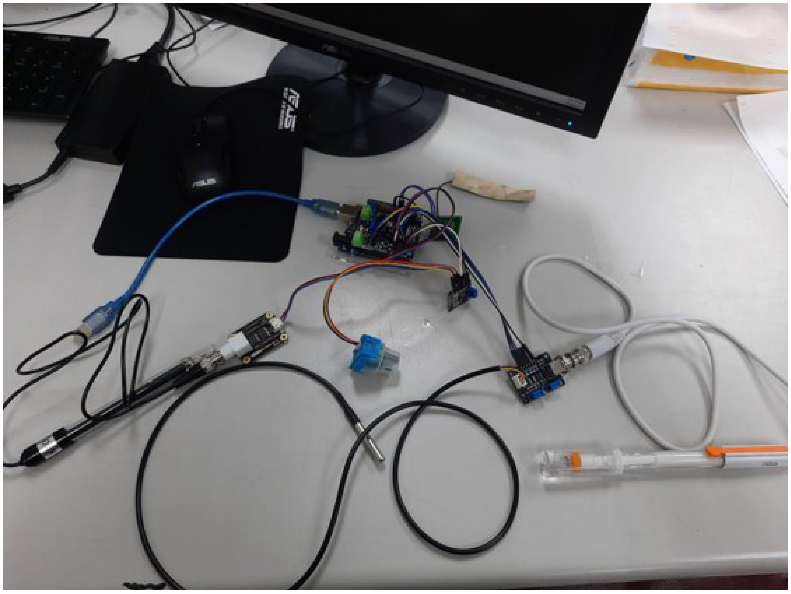
2.1. IoT Sensor Packages for Water Quality Monitoring
2.1.1. TDS Sensor
2.1.2. pH Sensor
2.1.3. DO Sensor
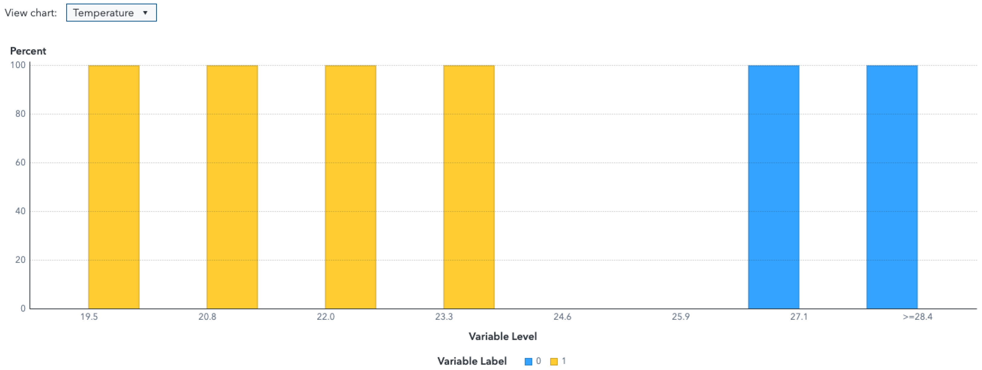
2.1.4. Temperature Sensor
2.1.5. NB-IoT
2.2. Machine Learning Models
2.2.1. DT
2.2.2. SVM
2.2.3. RF
2.2.4. Evaluation Model
3. Results
4. Discussion
5. Conclusions
Author Contributions
Funding
Institutional Review Board Statement
Informed Consent Statement
Data Availability Statement
Conflicts of Interest
References
- Al Jazeera Staff. Infographic: Which Countries Have the Safest Drinking Water? 2022. Available online: https://www.aljazeera.com/news/2022/3/22/infographic-which-countries-have-the-safest-drinking-water-interactive (accessed on 16 September 2023).
- World Health Organization (WHO). Drinking Water; World Health Organization (WHO): Geneva, Switzerland, 2002.
- Chhipi-Shrestha, G.; Mian, H.R.; Mohammadiun, S.; Rodriguez, M.; Hewage, K.; Sadiq, R. Digital water: Artificial intelligence and soft computing applications for drinking water quality assessment. Clean Technol. Environ. Policy 2023, 25, 1409–1438. [Google Scholar] [CrossRef]
- World Health Organization (WHO). Guidelines for Drinking-Water Quality, 4th ed.; World Health Organization (WHO): Geneva, Switzerland, 2017.
- Khan, M.S.I.; Islam, N.; Uddin, J.; Islam, S.; Nasir, M.K. Water quality prediction and classification based on principal component regression and gradient boosting classifier approach. J. King Saud Univ. Comput. Inf. Sci. 2022, 34, 4773–4781. [Google Scholar] [CrossRef]
- Abidin, Z.; Maulana, E.; Nurrohman, M.Y.; Wardana, F.C.; Warsito. Real Time Monitoring System of Drinking Water Quality Using Internet of Things. In Proceedings of the 2022 International Electronics Symposium (IES), Surabaya, Indonesia, 9–11 August 2022; Institute of Electrical and Electronics Engineers Inc.: Piscataway, NJ, USA, 2022; pp. 131–135. [Google Scholar] [CrossRef]
- Memon, A.R.; Memon, S.K.; Memon, A.A.; Memon, T.D. IoT Based Water Quality Monitoring System for Safe Drinking Water in Pakistan. In Proceedings of the 2020 3rd International Conference on Computing, Mathematics and Engineering Technologies (iCoMET), IEEE, Sukkur, Pakistan, 29–30 January 2020. [Google Scholar]
- Quinn, J.; Kabir, T.; Altaf, M.; Sawyer, L.; Wang, Y.; Choudhury, M.; Lee, J. H2O: Smart Drinking Water Quality Monitoring System. In Proceedings of the 2022 IEEE International Conference on Imaging Systems and Techniques (IST), Kaohsiung, Taiwan, 21–23 June 2022; Institute of Electrical and Electronics Engineers Inc.: Piscataway, NJ, USA, 2022; Volume 2022. [Google Scholar] [CrossRef]
- Al-Khashab, Y.; Daoud, R.; Yasen, M.; Majeed, M. Drinking Water Monitoring in Mosul City Using IoT. In Proceedings of the 2019 International Conference on Computing and Information Science and Technology and Their Applications (ICCISTA), Kirkuk, Iraq, 3–5 March 2019. [Google Scholar]
- Irawan, Y.; Febriani, A.; Wahyuni, R.; Devis, Y. Water Quality Measurement and Filtering Tools Using Arduino Uno, PH Sensor and TDS Meter Sensor. J. Robot. Control. (JRC) 2021, 2, 357–362. [Google Scholar] [CrossRef]
- Ryu, J.H. UAS-based real-time water quality monitoring, sampling, and visualization platform (UASWQP). HardwareX 2022, 11, e00277. [Google Scholar] [CrossRef]
- Ryu, J.H. Prototyping a low-cost open-source autonomous unmanned surface vehicle for real-time water quality monitoring and visualization. HardwareX 2022, 12, e00369. [Google Scholar] [CrossRef]
- Sihwi, S.W.; Fikri, K.; Aziz, A. Dysgraphia Identification from Handwriting with Support Vector Machine Method. J. Phys. Conf. Ser. 2019, 1201, 012050. [Google Scholar] [CrossRef]
- Cervantes, J.; Garcia-Lamont, F.; Rodríguez-Mazahua, L.; Lopez, A. A comprehensive survey on support vector machine classification: Applications, challenges and trends. Neurocomputing 2020, 408, 189–215. [Google Scholar] [CrossRef]
- Aldhyani, T.H.; Al-Yaari, M.; Alkahtani, H.; Maashi, M. Water Quality Prediction Using Artificial Intelligence Algorithms. Appl. Bionics Biomech. 2020, 2020, 6659314. [Google Scholar] [CrossRef]
- Nasir, N.; Kansal, A.; Alshaltone, O.; Barneih, F.; Sameer, M.; Shanableh, A.; Al-Shamma’a, A. Water quality classification using machine learning algorithms. J. Water Process. Eng. 2022, 48, 102920. [Google Scholar] [CrossRef]
- Xue, P.; Lei, Y.; Li, Y. Research and prediction of Shanghai-Shenzhen 20 Index Based on the Support Vector Machine Model and Gradient Boosting Regression Tree. In Proceedings of the 2020 International Conference on Intelligent Computing, Automation and Systems (ICICAS), Chongqing, China, 11–13 December 2020; Institute of Electrical and Electronics Engineers Inc.: Piscataway, NJ, USA, 2020; Volume 12, pp. 58–62. [Google Scholar] [CrossRef]
- Reddy, P.V.; Kumar, S.M. A Method for Determining the Accuracy of Stock Prices using Gradient Boosting and the Support Vector Machines Algorithm. In Proceedings of the 2022 3rd International Conference on Smart Electronics and Communication (ICOSEC), Trichy, India, 20–22 October 2022; Institute of Electrical and Electronics Engineers Inc.: Piscataway, NJ, USA, 2022; pp. 1596–1599. [Google Scholar] [CrossRef]
- Mitrofanov, S.; Semenkin, E. An approach to training decision trees with the relearning of nodes. In Proceedings of the 2021 International Conference on Information Technologies (InfoTech), Varna, Bulgaria, 16–17 September 2021; Institute of Electrical and Electronics Engineers Inc.: Piscataway, NJ, USA, 2021; Volume 9. [Google Scholar] [CrossRef]
- Santos, L.I.; Camargos, M.O.; D’Angelo, M.F.S.V.; Mendes, J.B.; de Medeiros, E.E.C.; Guimarães, A.L.S.; Palhares, R.M. Decision tree and artificial immune systems for stroke prediction in imbalanced data. Expert Syst. Appl. 2022, 191, 116221. [Google Scholar] [CrossRef]
- Bouquet, A.; Laabir, M.; Rolland, J.L.; Chomérat, N.; Reynes, C.; Sabatier, R.; Felix, C.; Berteau, T.; Chiantella, C.; Abadie, E. Prediction of Alexandrium and Dinophysis algal blooms and shellfish contamination in French Mediterranean Lagoons using decision trees and linear regression: A result of 10 years of sanitary monitoring. Harmful Algae 2022, 115, 102234. [Google Scholar] [CrossRef]
- Ajayi, O.O.; Bagula, A.B.; Maluleke, H.C.; Gaffoor, Z.; Jovanovic, N.; Pietersen, K.C. WaterNet: A Network for Monitoring and Assessing Water Quality for Drinking and Irrigation Purposes. IEEE Access 2022, 10, 48318–48337. [Google Scholar] [CrossRef]
- Hong, M.; Kim, K.; Hwang, Y. Arduino and IoT-based direct filter observation method monitoring the color change of water filter for safe drinking water. J. Water Process. Eng. 2022, 49, 103158. [Google Scholar] [CrossRef]
- Huang, S.; Nianguang, C.A.; Pacheco, P.P.; Narandes, S.; Wang, Y.; Wayne, X.U. Applications of support vector machine (SVM) learning in cancer genomics. Cancer Genom. Proteom. 2018, 15, 41–51. [Google Scholar] [CrossRef]
- Chiu, M.C.; Yan, W.M.; Bhat, S.A.; Huang, N.F. Development of smart aquaculture farm management system using IoT and AI-based surrogate models. J. Agric. Food Res. 2022, 9, 100357. [Google Scholar] [CrossRef]
- Liu, Y.; Zhang, Q.; Song, L.; Chen, Y. Attention-based recurrent neural networks for accurate short-term and long-term dissolved oxygen prediction. Comput. Electron. Agric. 2019, 165, 104964. [Google Scholar] [CrossRef]
- Das, B.; Jain, P.C. IoT based Real-Time Water Quality Monitoring System using smart Sensors. Int. Res. J. Eng. Technol. 2020, 2020, 181–186. [Google Scholar]
- Popli, S.; Jha, R.K.; Jain, S. A Survey on Energy Efficient Narrowband Internet of Things (NBIoT): Architecture, Application and Challenges. IEEE Access 2019, 7, 16739–16776. [Google Scholar] [CrossRef]
- Huan, J.; Li, H.; Wu, F.; Cao, W. Design of water quality monitoring system for aquaculture ponds based on NB-IoT. Aquac. Eng. 2020, 90, 102088. [Google Scholar] [CrossRef]
- Zhu, M.; Wang, J.; Yang, X.; Zhang, Y.; Zhang, L.; Ren, H.; Wu, B.; Ye, L. A review of the application of machine learning in water quality evaluation. Eco-Environ. Health 2022, 1, 107–116. [Google Scholar] [CrossRef] [PubMed]


| Authors | Prediction Approach | Results |
|---|---|---|
| Aldhyani [15] | SVM, Naive Bayes, K-nearest neighbor | SVM had the highest percentage accuracy of 97.01 |
| Nasir [16] | SVM, LR, RF, DT, CATBoost, MLP, XGBoost | CATBoost had the highest percentage accuracy of 94.51 |
| Khan [5] | LR, GB, RF, SVM | GB had the highest percentage accuracy of 100 |
| Parameter | Training | Validation | Testing |
|---|---|---|---|
| Accuracy | 0.9665 | 0.9753 | 0.9754 |
| Error | 0.0335 | 0.0247 | 0.0246 |
| Sensitivity | 0.9978 | 0.9978 | 0.9935 |
| Specificity | 0.9294 | 0.9486 | 0.9538 |
| Parameter | DT | RF | GB | SVM | NN |
|---|---|---|---|---|---|
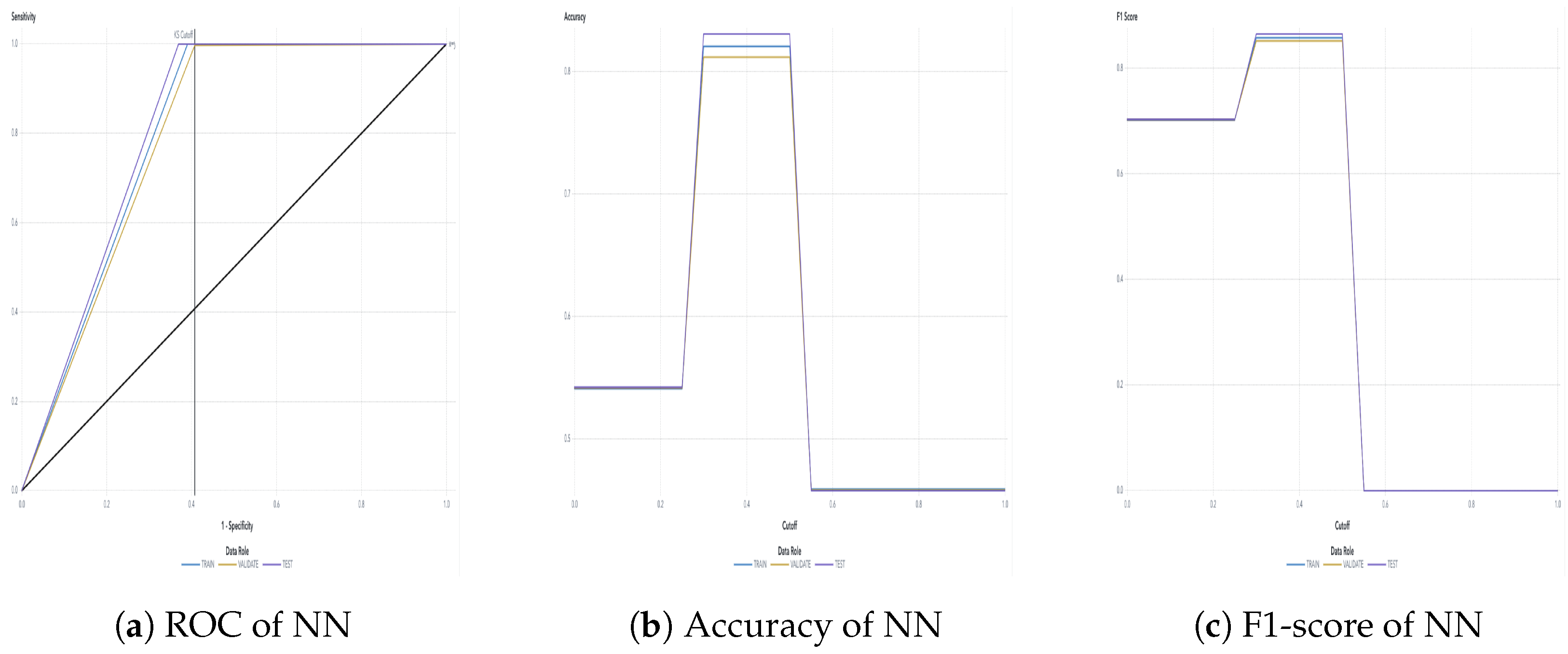
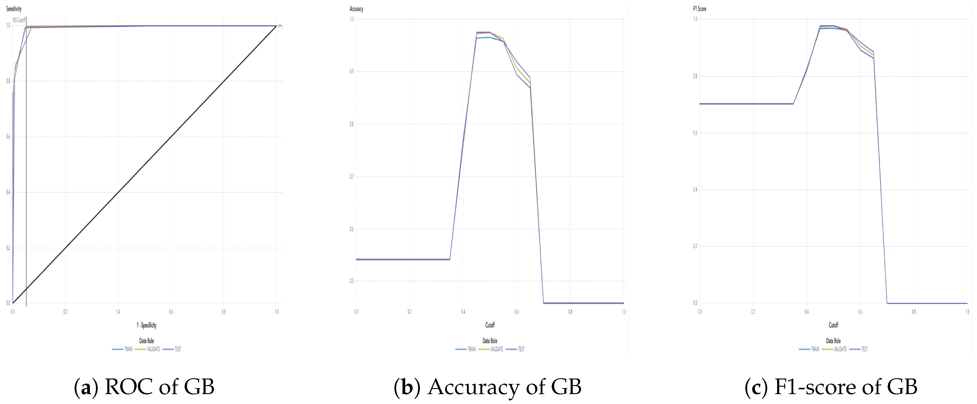
| Accuracy | 0.97887 | 0.97535 | 0.97535 | 0.97535 | 0.83099 |
| F1-Score | 0.98077 | 0.97764 | 0.97764 | 0.97764 | 0.8652 |
| ROC | 0.99213 | 0.99505 | 0.99303 | 0.98442 | 0.81538 |
Disclaimer/Publisher’s Note: The statements, opinions and data contained in all publications are solely those of the individual author(s) and contributor(s) and not of MDPI and/or the editor(s). MDPI and/or the editor(s) disclaim responsibility for any injury to people or property resulting from any ideas, methods, instructions or products referred to in the content. |
© 2024 by the authors. Licensee MDPI, Basel, Switzerland. This article is an open access article distributed under the terms and conditions of the Creative Commons Attribution (CC BY) license (https://creativecommons.org/licenses/by/4.0/).
Share and Cite
Wiryasaputra, R.; Huang, C.-Y.; Lin, Y.-J.; Yang, C.-T. An IoT Real-Time Potable Water Quality Monitoring and Prediction Model Based on Cloud Computing Architecture. Sensors 2024, 24, 1180. https://doi.org/10.3390/s24041180
Wiryasaputra R, Huang C-Y, Lin Y-J, Yang C-T. An IoT Real-Time Potable Water Quality Monitoring and Prediction Model Based on Cloud Computing Architecture. Sensors. 2024; 24(4):1180. https://doi.org/10.3390/s24041180
Chicago/Turabian StyleWiryasaputra, Rita, Chin-Yin Huang, Yu-Ju Lin, and Chao-Tung Yang. 2024. "An IoT Real-Time Potable Water Quality Monitoring and Prediction Model Based on Cloud Computing Architecture" Sensors 24, no. 4: 1180. https://doi.org/10.3390/s24041180