
A Snapshot Multi-Spectral Demosaicing Method for Multi-Spectral Filter Array Images Based on Channel Attention Network
Abstract
:1. Introduction
1.1. Background
1.2. Related Works
1.3. Our Contribution
- We analyze the acquisition process of multi-spectral images, laying the theoretical groundwork for synthesizing the mosaic images and the radiance label images using the spectral sensitive functions (SSFs) of the IMEC camera we purchased and the available illuminants.
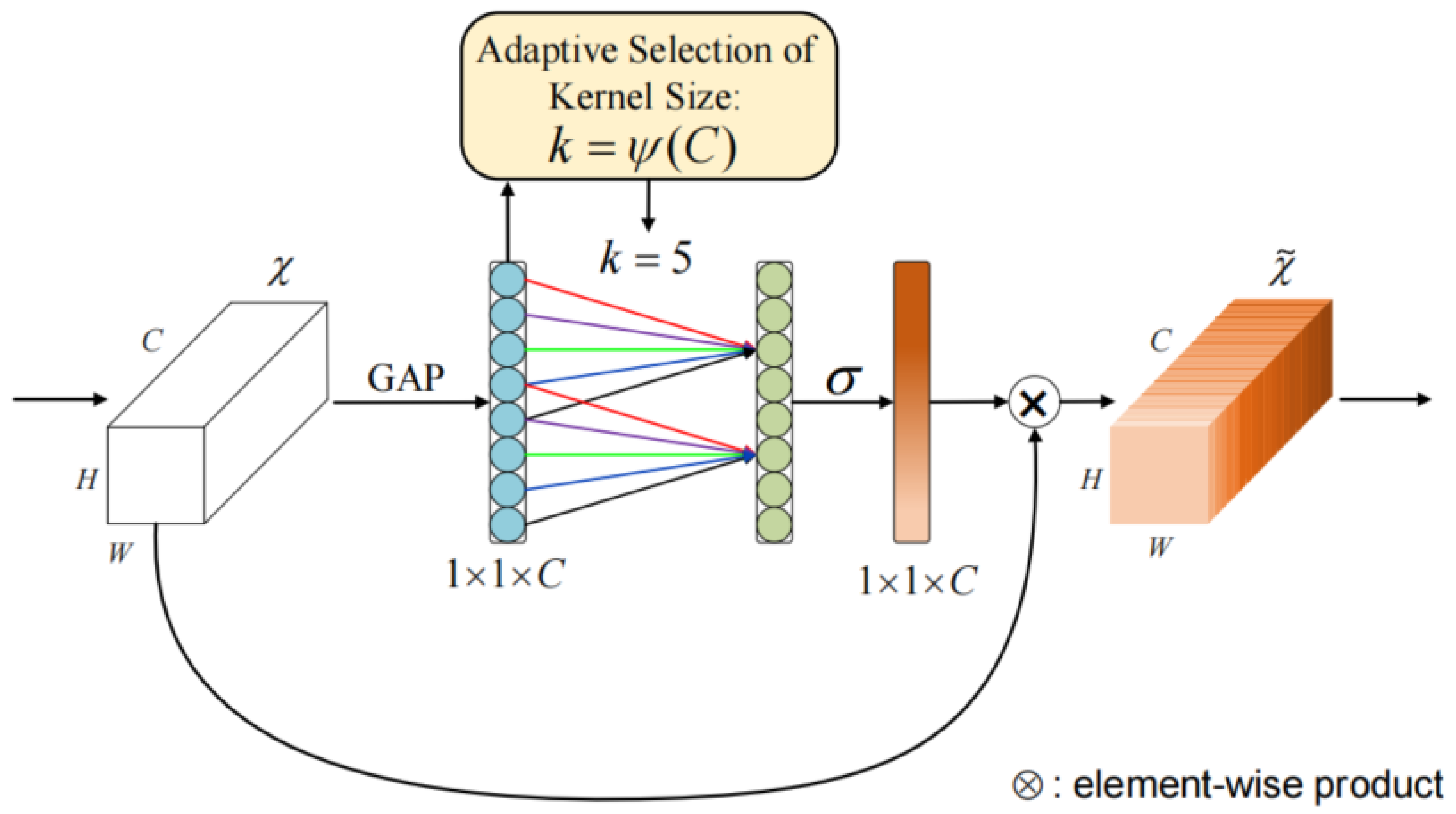
- We present a simple and feasible end-to-end deep convolution neural network that introduces the channel attention mechanism, which is able to adaptively adjust channel feature response and protect important channel features.
- The methodology we propose exhibits superior demosaicing performance on both simulated datasets and real-world scenarios compared to other existing methods, offering significant potential for the application of IMEC’s camera in both commercial and industrial sectors.
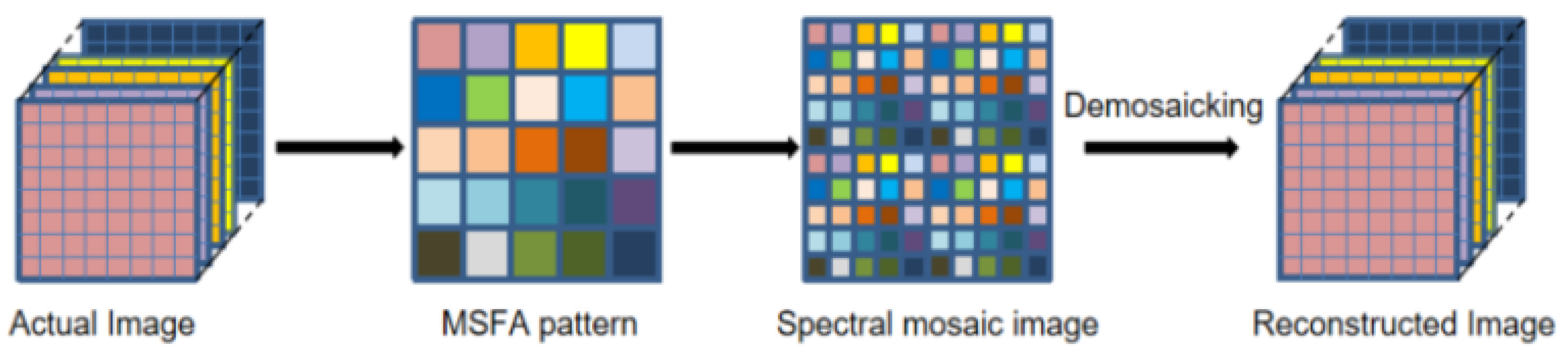
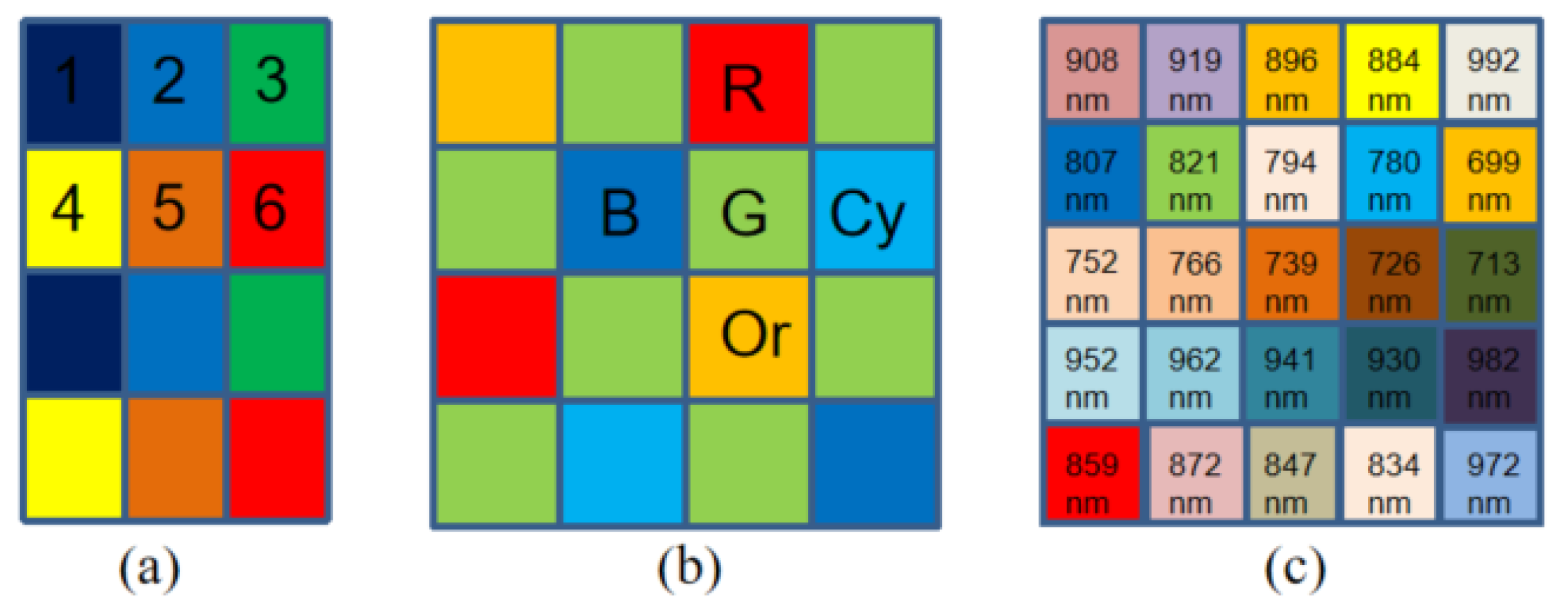
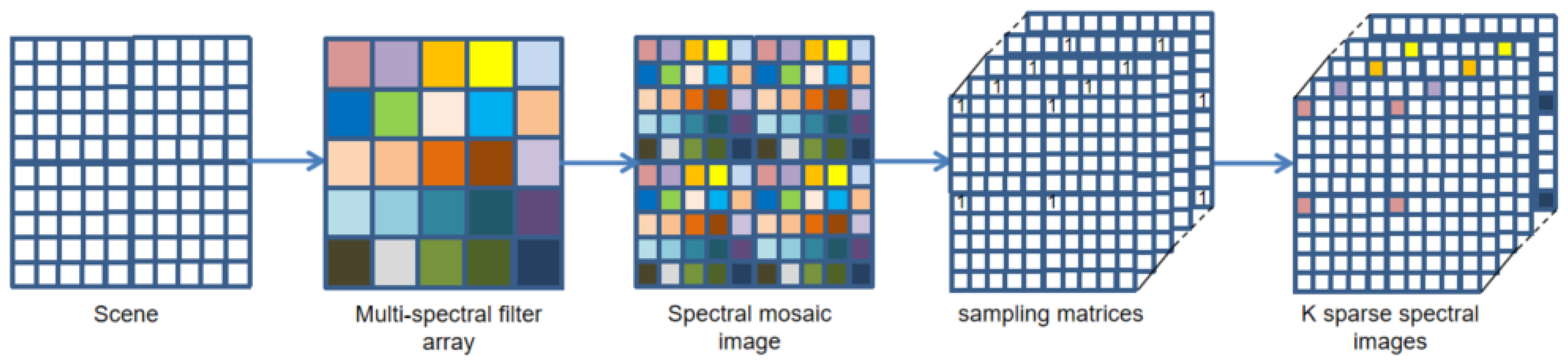
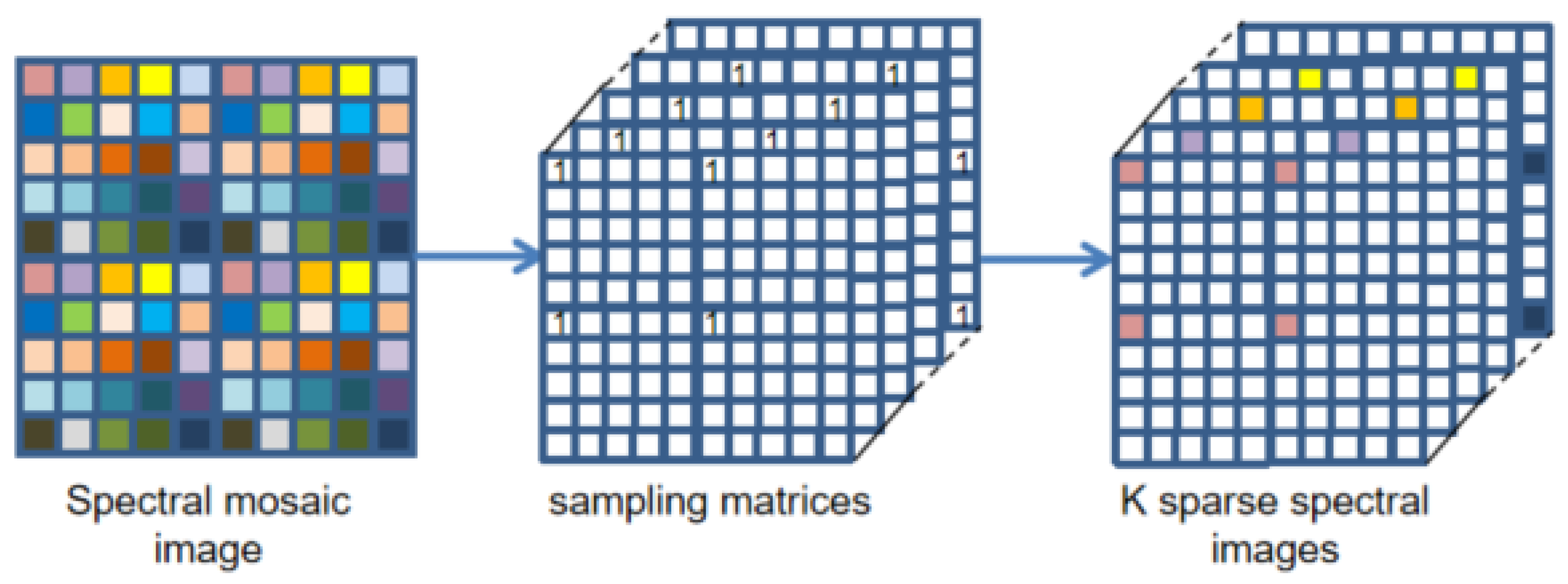
2. Observation Model
3. Reference Image Simulation
3.1. Multi-Spectral Image Formation
3.2. Simulation of Radiance Data
3.3. Multi-Spectral Image Simulation
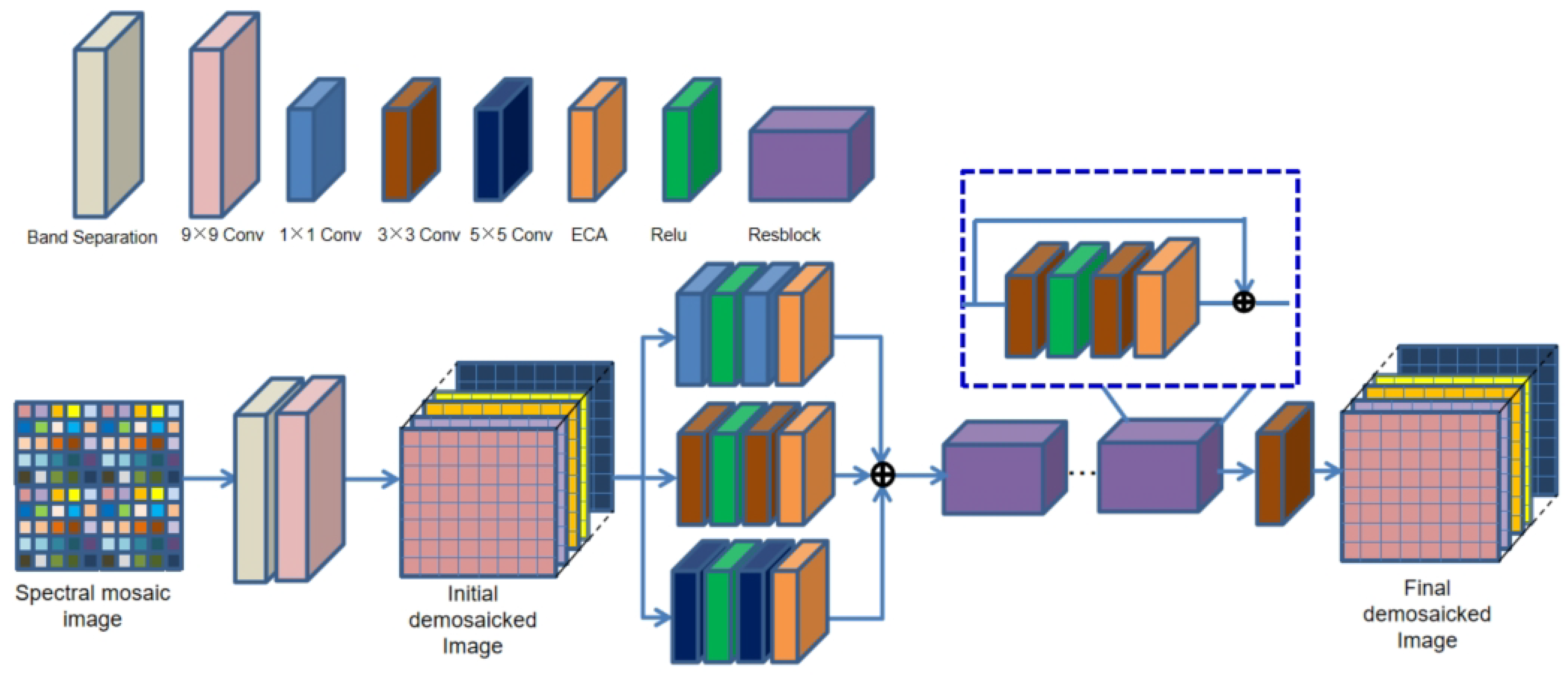
4. Proposed Demosaicing Method
4.1. Network Framework
4.2. Loss Function
5. Datasets and Training
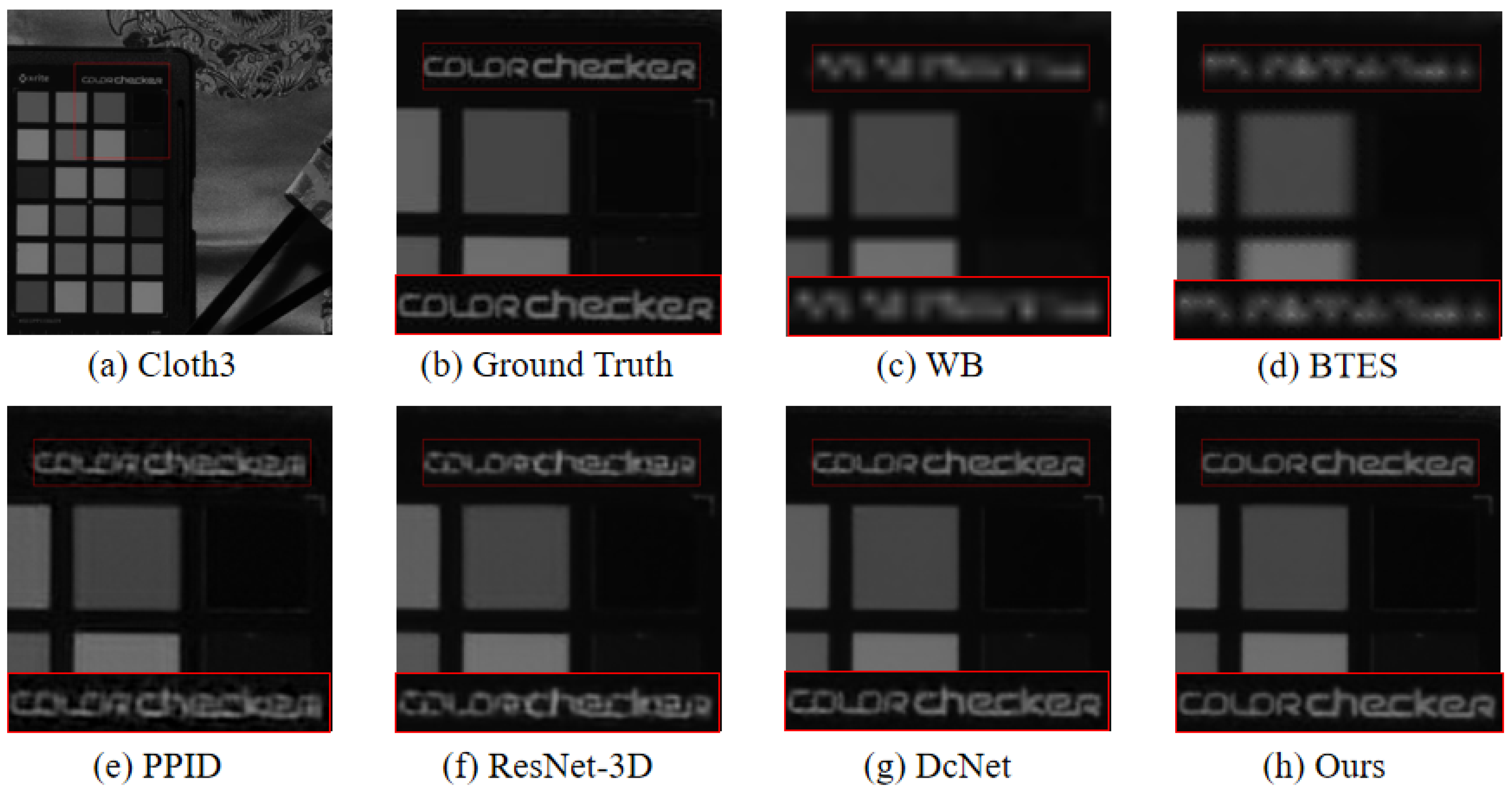
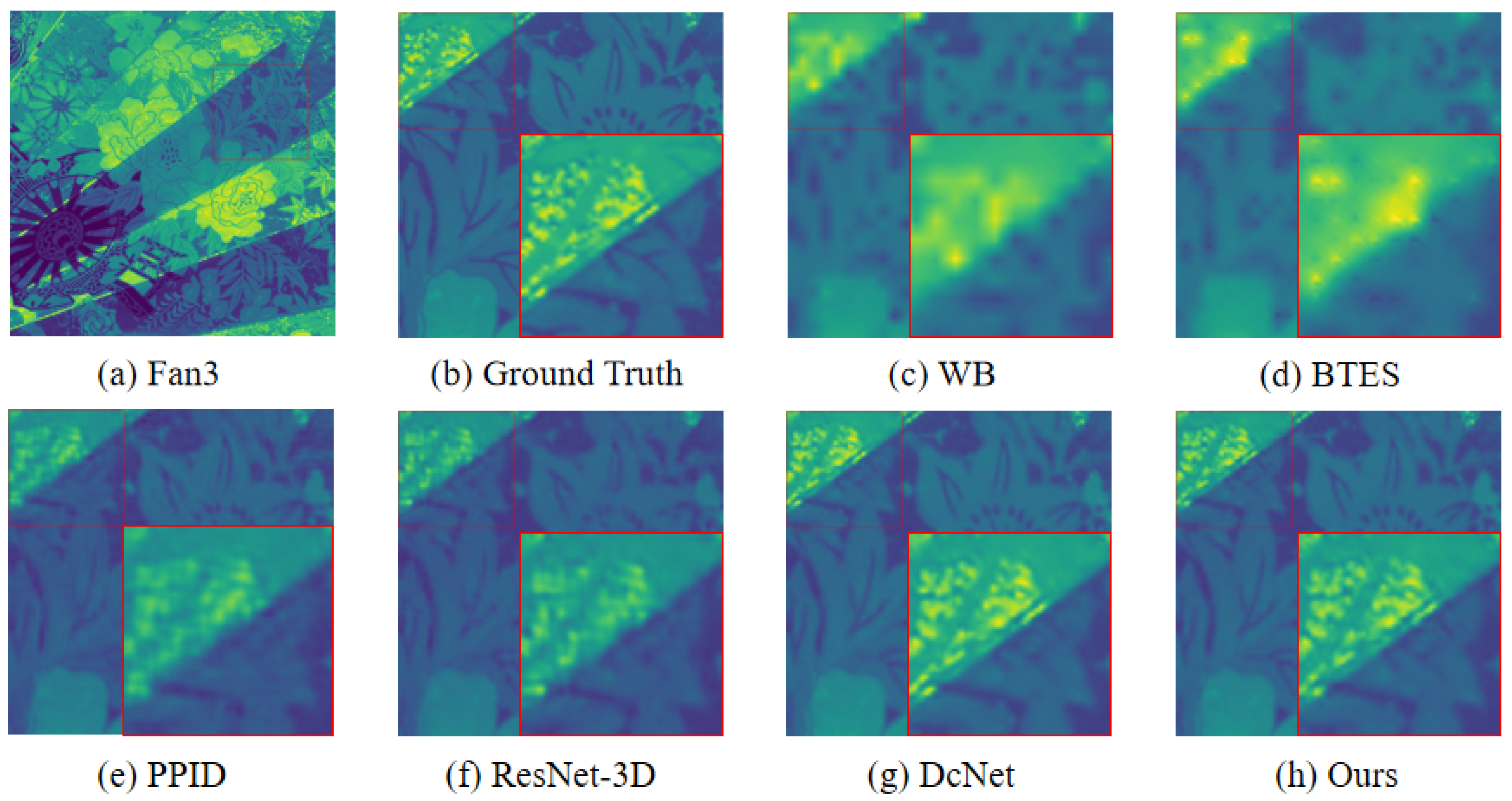
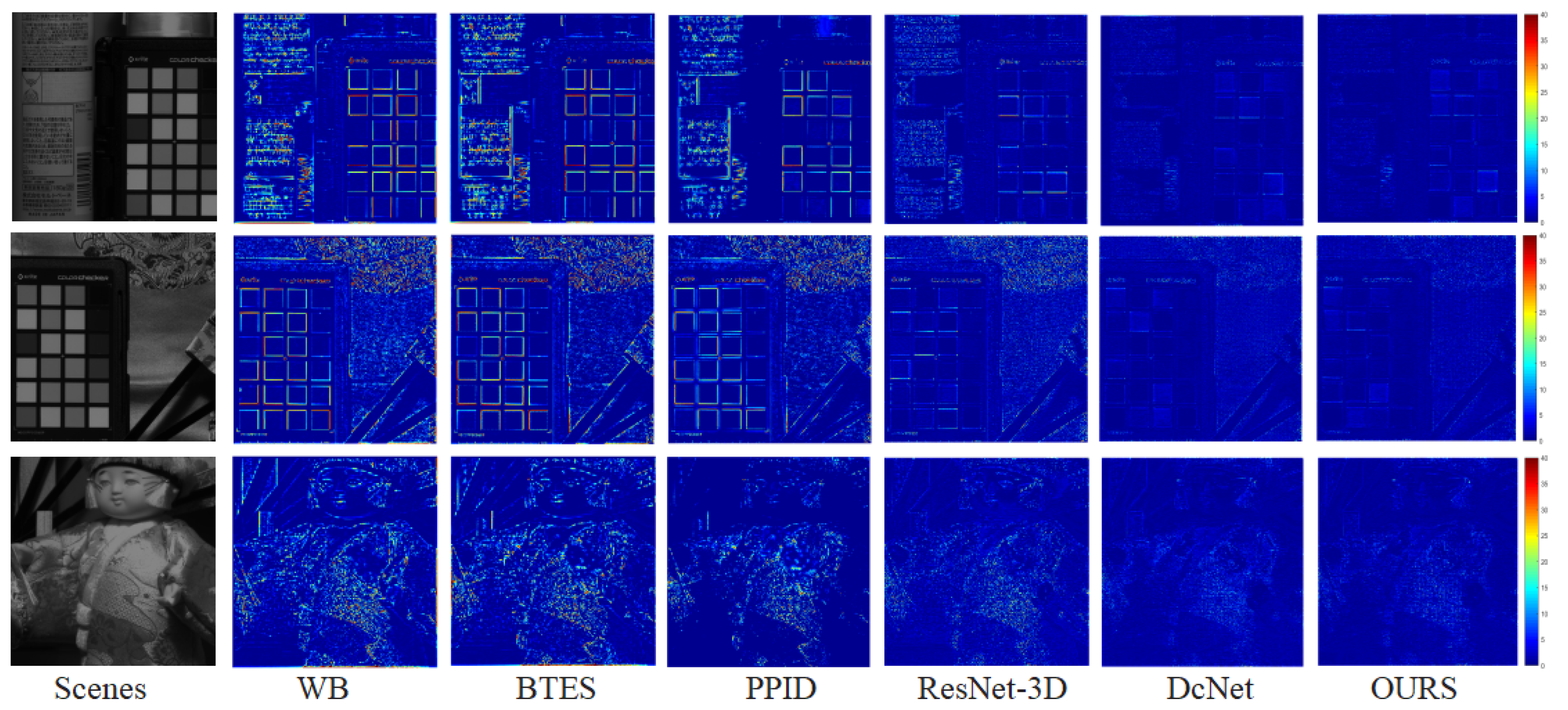
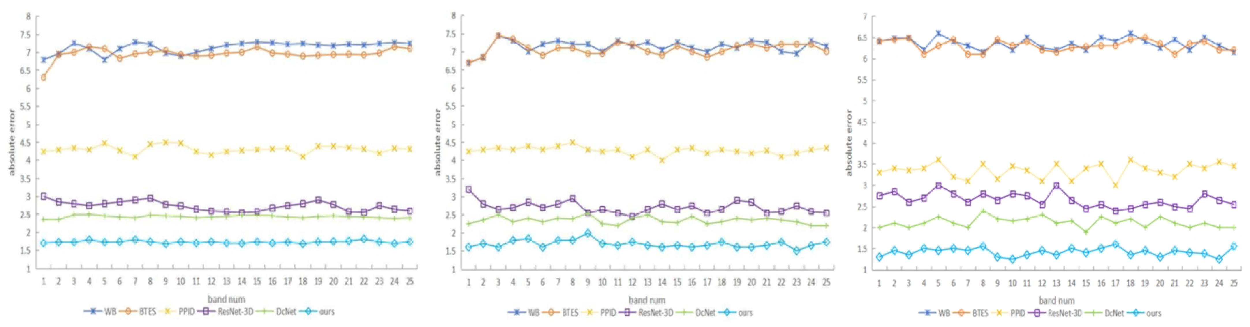
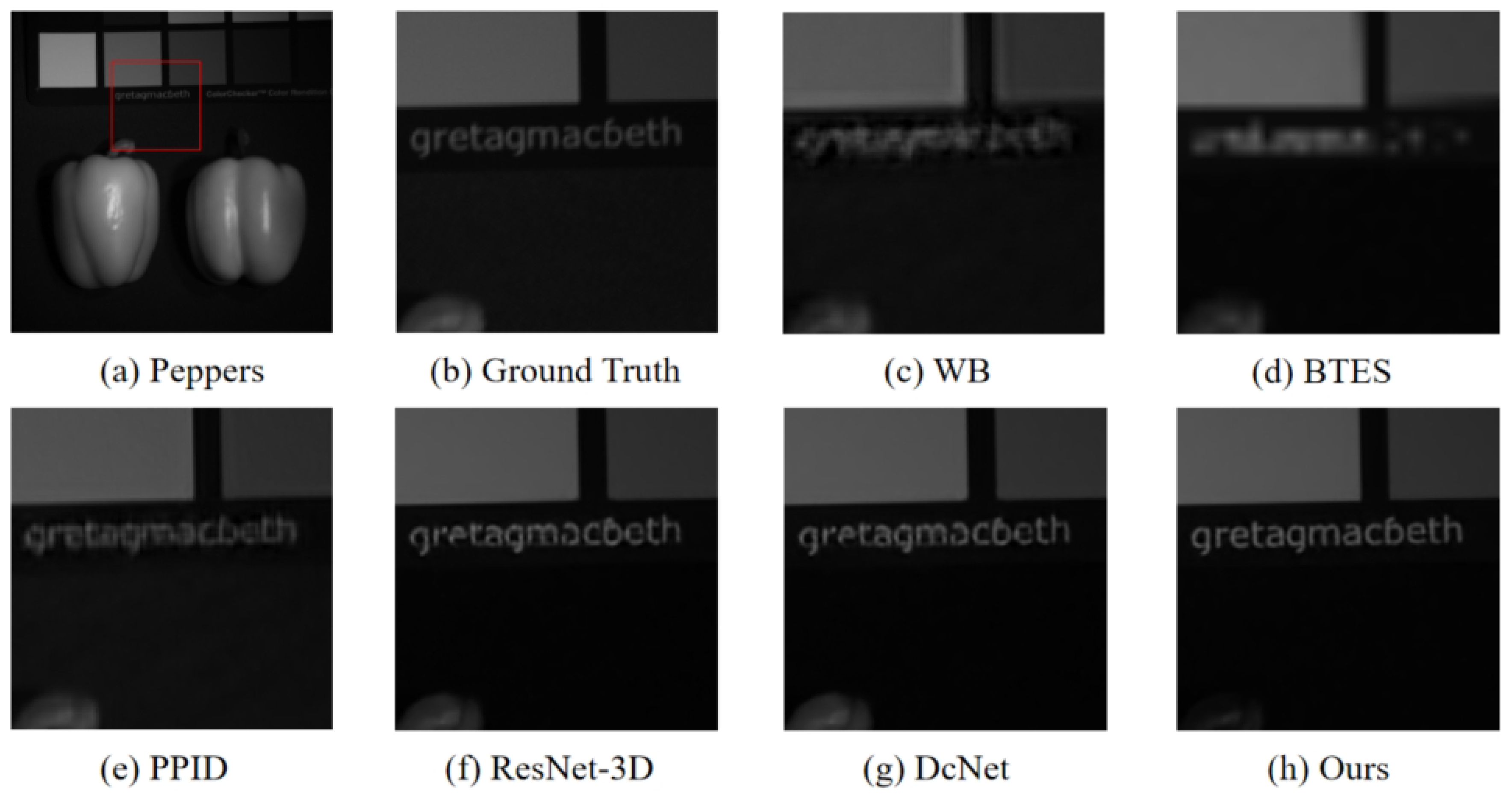
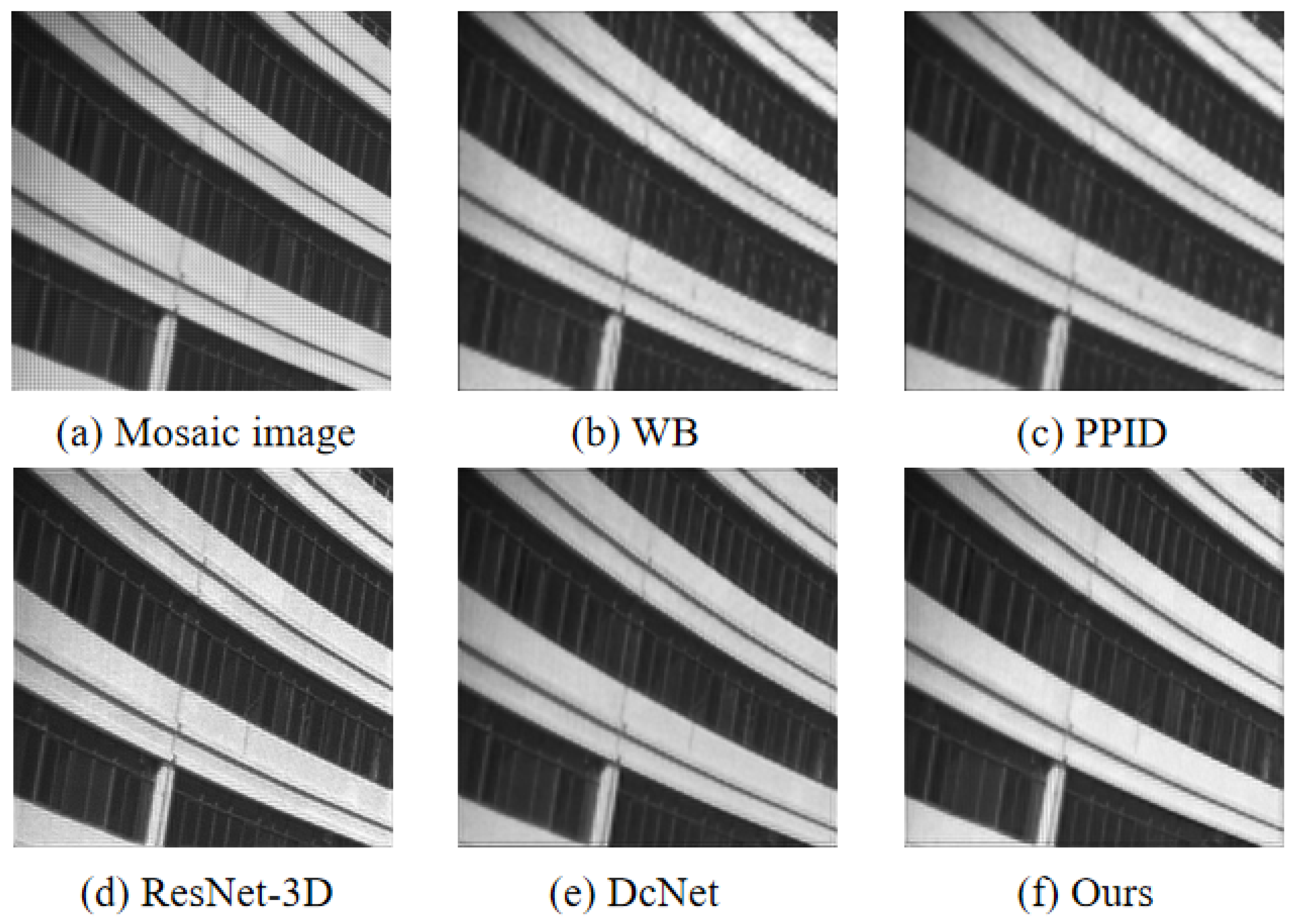
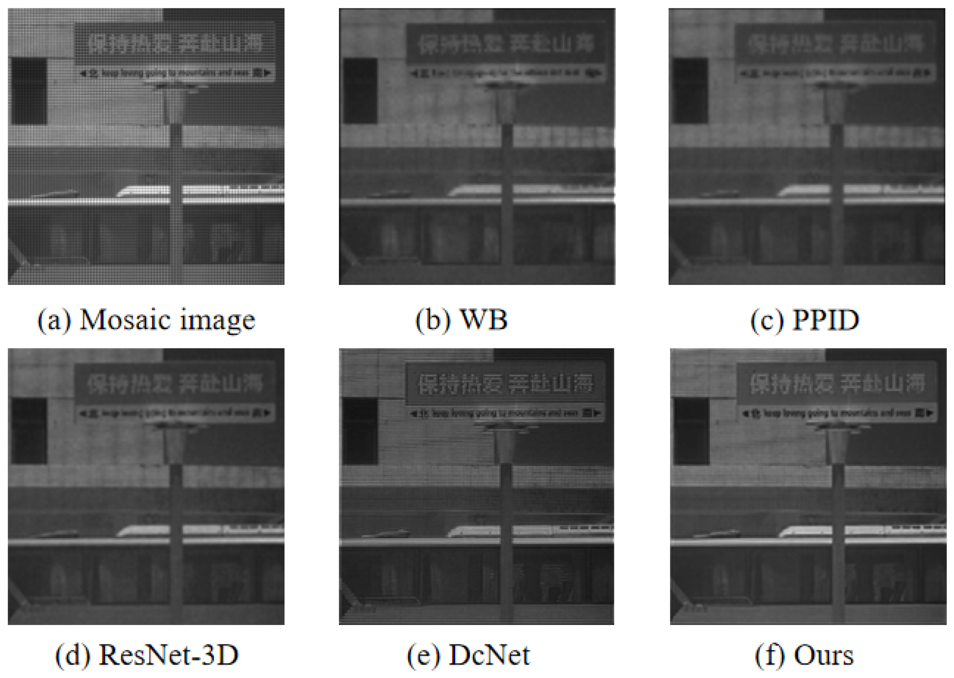
6. Experimental Results with Simulated Data and Real-Word Data
7. Discussion
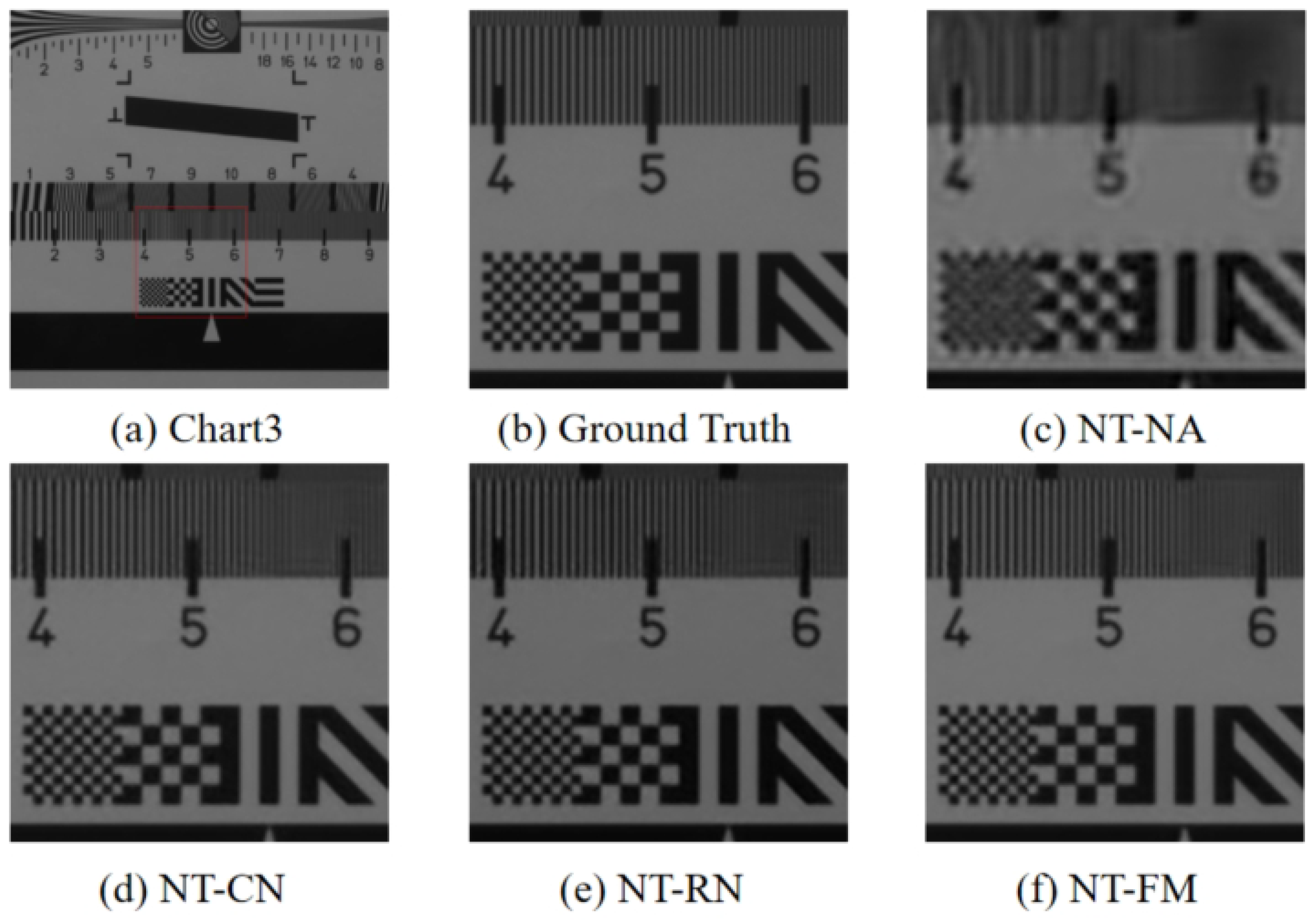
8. Ablation Studies
- (1)
- The base model without any attention, labeled as NT-NA;
- (2)
- The base model with ECA added to the convolutional network, labeled as NT-CN;
- (3)
- The base model with ECA added to the residual network, labeled as NT-RN;
- (4)
- The base model with ECA, which is our full model, is labeled as NT-FM.
9. Conclusions
Author Contributions
Funding
Institutional Review Board Statement
Informed Consent Statement
Data Availability Statement
Conflicts of Interest
References
- Pu, H.; Lin, L.; Sun, D.W. Principles of hyperspectral microscope imaging techniques and their applications in food quality and safety detection: A review. Compr. Rev. Food Sci. Food Saf. 2019, 18, 853–866. [Google Scholar] [CrossRef]
- Hashimoto, E. Tissue classifification of liver pathological tissue specimens image using spectral features. Proc. SPIE 2017, 10140, 101400Z. [Google Scholar] [CrossRef]
- Hadoux, X.; Gorretta, N.; Roger, J.M.; Bendoula, R.; Rabatel, G. Comparison of the efficacy of spectral pre-treatments for wheat and weed discrimination in outdoor conditions. Comput. Electron. Agric. 2014, 108, 242–249. [Google Scholar] [CrossRef]
- Uzkent, B.; Rangnekar, A.; Hoffman, M.J. Tracking in aerial hyperspectral videos using deep kernelized correlation filters. IEEE Trans. Geosci. Remote Sens. 2019, 57, 449–461. [Google Scholar] [CrossRef]
- Xiong, F.; Zhou, J.; Qian, Y. Material based object tracking in hyperspectral videos. IEEE Trans. Image Process. 2020, 29, 3719–3733. [Google Scholar] [CrossRef] [PubMed]
- Chi, C.; Yoo, H.; Ben-Ezra, M. Multi-spectral imaging by optimized wide band illumination. Int. J. Comput. Vis. 2010, 86, 140–151. [Google Scholar] [CrossRef]
- Ohsawa, K.; Ajito, T.; Komiya, Y.; Fukuda, H.; Haneishi, H.; Yamaguchi, M.; Ohyama, N. Six-band HDTV camera system for spectrum-based color reproduction. J. Imaging Sci. Technol. 2004, 48, 85–92. [Google Scholar] [CrossRef]
- Lapray, P.J.; Wang, X.; Thomas, J.B.; Gouton, P. Multispectral filter arrays: Recent advances and practical implementation. Sensors 2014, 14, 21626–21659. [Google Scholar] [CrossRef]
- Geelen, B.; Tack, N.; Lambrechts, A. A compact snapshot multispectral imager with a monolithically integrated per-pixel filter mosaic. Proc. SPIE 2014, 8974, 80–87. [Google Scholar] [CrossRef]
- Martínez, M.A.; Valero, E.M.; Hernández-Andrés, J.; Romero, J.; Langfelder, G. Combining transverse field detectors and color filter arrays to improve multispectral imaging systems. Appl. Opt. 2014, 53, C14–C24. [Google Scholar] [CrossRef]
- Monno, Y.; Kikuchi, S.; Tanaka, M.; Okutomi, M. A practical one-shot multispectral imaging system using a single image sensor. IEEE Trans. Image Process. 2015, 24, 3048–3059. [Google Scholar] [CrossRef]
- Thomas, J.B.; Lapray, P.J.; Gouton, P.; Clerc, C. Spectral characterization of a prototype SFA camera for joint visible and NIR acquisition. Sensors 2016, 16, 993. [Google Scholar] [CrossRef] [PubMed]
- Murakami, Y.; Yamaguchi, M.; Ohyama, N. Spectral Hybrid-resolution multispectral imaging using color filter array. Opt. Express 2012, 20, 7173–7183. [Google Scholar] [CrossRef]
- Jaiswal, S.P.; Fang, L.; Jakhetiya, V.; Pang, J.; Mueller, K.; Au, O.C. Adaptive multispectral demosaicing based on frequency domain analysis of spectral correlation. IEEE Trans. Image Process. 2017, 26, 953–968. [Google Scholar] [CrossRef]
- Fukuda, H.; Uchiyama, T.; Haneishi, H.; Yamaguchi, M.; Ohyama, N. Development of a 16-band multispectral image archiving system. In Proceedings of the SPIE Electronic Imaging: Color Imaging X, San Jose, CA, USA, 17–20 January 2005; Volume 5667, pp. 136–145. [Google Scholar] [CrossRef]
- Monakhova, K.; Yanny, K.; Aggarwal, N.; Waller, L. Spectral DiffuserCam: Lensless snapshot hyperspectral imaging with a spectral filter array. Optica 2020, 7, 1298–1307. [Google Scholar] [CrossRef]
- Gunturk, B.K.; Glotzbach, J.; Altunbasak, Y.; Schafer, R.W.; Mersereau, R.M. Demosaicing: Color filter array interpolation. IEEE Signal Process. Mag. 2005, 22, 44–54. [Google Scholar] [CrossRef]
- Monno, Y.; Tanaka, M.; Okutomi, M. Multispectral demosaicing using guided filter. Digit. Photogr. VIII 2012, 8299, 204–210. [Google Scholar] [CrossRef]
- Zhao, B.; Zheng, J.; Dong, Y.; Shen, N.; Yang, J.; Cao, Y.; Cao, Y. PPI Edge Infused Spatial–Spectral Adaptive Residual Network for Multispectral Filter Array Image Demosaicing. IEEE Trans. Geosci. Remote Sens. 2023, 61, 1–14. [Google Scholar] [CrossRef]
- Rathi, V.; Goyal, P. Generic multispectral demosaicking using spectral correlation between spectral bands and pseudo-panchromatic image. Signal Process. Image Commun. 2023, 110, 116893. [Google Scholar] [CrossRef]
- Gupta, M.; Rathi, V.; Goyal, P. Adaptive and Progressive Multispectral Image Demosaicking. IEEE Trans. Comput. Imaging 2022, 8, 69–80. [Google Scholar] [CrossRef]
- Brauers, J.; Aach, T. A Color Filter Array based Multispectral Camera. In Proceedings of the Workshop Farbbildverarbeitung, Ilmenau, Germany, 5–6 October 2006. [Google Scholar]
- Wang, X.; Thomas, J.B.; Hardeberg, J.Y.; Gouton, P. Discrete wavelet transform based multispectral filter array demosaicing. In Proceedings of the 2013 Colour and Visual Computing Symposium (CVCS), Gjovik, Norway, 5–6 September 2013; pp. 1–6. [Google Scholar] [CrossRef]
- Driesen, J.; Scheunders, P. Wavelet-based color filter array demosaicing. In Proceedings of the International Conference on Image Processing (ICIP), Singapore, 24–27 October 2004; Volume 5, pp. 3311–3314. [Google Scholar] [CrossRef]
- Miao, L.; Qi, H.; Ramanath, R.; Snyder, W.E. Binary tree-based generic demosaicing algorithm for multispectral filter arrays. IEEE Trans. Image Process. 2006, 15, 3550–3558. [Google Scholar] [CrossRef]
- Mihoubi, S.; Losson, O.; Mathon, B.; Macaire, L. Multispectral demosaicing using pseudo-panchromatic image. IEEE Trans. Comput. Imaging 2017, 3, 982–995. [Google Scholar] [CrossRef]
- Xu, L.; Ren, J.S.; Liu, C.; Jia, J. Deep convolutional neural network for image deconvolution. In Proceedings of the International Conference on Neural Information Processing Systems, Montreal, QC, Canada, 8–13 December 2014; pp. 1790–1798. [Google Scholar]
- Dong, C.; Loy, C.C.; He, K.; Tang, X. Learning a deep convolutional network for image super-resolution. In Proceedings of the European Conference on Computer Vision, Zurich, Switzerland, 6–12 September 2014; pp. 184–199. [Google Scholar] [CrossRef]
- Kim, J.; Lee, J.K.; Lee, K.M. Deeply-recursive convolutional network for image super-resolution. In Proceedings of the IEEE Conference on Computer Vision and Pattern Recognition, Las Vegas, NV, USA, 27–30 June 2016; pp. 1637–1645. [Google Scholar] [CrossRef]
- Wang, X.; Chen, J.; Wei, Q.; Richard, C. Hyperspectral image super resolution via deep prior regularization with parameter estimation. IEEE Trans. Circuits Syst. Video Technol. 2022, 32, 1708–1723. [Google Scholar] [CrossRef]
- Xu, Y.; Feng, K.; Yan, X.; Sheng, X.; Sun, B.; Liu, Z.; Yan, R. Cross-modal Fusion Convolutional Neural Networks with Online Soft Label Training Strategy for Mechanical Fault Diagnosis. IEEE Trans. Ind. Inform. 2023, 20, 73–84. [Google Scholar] [CrossRef]
- Xu, Y.; Feng, K.; Yan, X.; Yan, R.; Ni, Q.; Sun, B.; Lei, Z.; Zhang, Y.; Liu, Z. CFCNN: A novel convolutional fusion framework for collaborative fault identification of rotating machinery. Inf. Fusion 2023, 95, 1–16. [Google Scholar] [CrossRef]
- Xie, J.; Xu, L.; Chen, E. Image denoising and inpainting with deep neural networks. In Proceedings of the International Conference on Neural Information Processing Systems, Lake Tahoe, NV, USA, 3–6 December 2012; pp. 341–349. [Google Scholar]
- Zeng, X.; Bian, W.; Liu, W.; Shen, J.; Tao, D. Dictionary pair learning on Grassmann manifolds for image denoising. IEEE Trans. Image Process. 2015, 24, 4556–4569. [Google Scholar] [CrossRef] [PubMed]
- Pan, Z.; Li, B.; Cheng, H.; Bao, Y. Deep residual network for MSFA raw image denoising. In Proceedings of the IEEE International Conference on Acoustics, Speech and Signal Processing, Barcelona, Spain, 4–8 May 2020; pp. 2413–2417. [Google Scholar] [CrossRef]
- Cai, Y.; Lin, J.; Lin, Z.; Wang, H.; Zhang, Y.; Pfister, H.; Timofte, R.; Van Gool, L. Mst++: Multi-stage spectral-wise transformer for efficient spectral reconstruction. In Proceedings of the IEEE/CVF Conference on Computer Vision and Pattern Recognition, New Orleans, LA, USA, 19–20 June 2022; pp. 745–755. [Google Scholar] [CrossRef]
- Shi, Z.; Chen, C.; Xiong, Z.; Liu, D.; Wu, F. Hscnn+: Advanced cnn-based hyperspectral recovery from rgb images. In Proceedings of the IEEE Conference on Computer Vision and Pattern Recognition Workshops, Salt Lake City, UT, USA, 18–22 June 2018; pp. 939–947. [Google Scholar] [CrossRef]
- Li, J.; Wu, C.; Song, R.; Li, Y.; Liu, F. Adaptive weighted attention network with camera spectral sensitivity prior for spectral reconstruction from RGB images. In Proceedings of the IEEE Conference on Computer Vision and Pattern Recognition Workshops, Seattle, WA, USA, 14–19 June 2020; pp. 462–463. [Google Scholar] [CrossRef]
- Shinoda, K.; Yoshiba, S.; Hasegawa, M. Deep demosaicing for multispectral filter arrays. arXiv 2018, arXiv:1808.08021. [Google Scholar]
- Wisotzky, E.L.; Daudkane, C.; Hilsmann, A.; Eisert, P. Hyperspectral Demosaicing of Snapshot Camera Images Using Deep Learning. In Proceedings of the DAGM German Conference on Pattern Recognition, Konstanz, Germany, 27–30 September 2022; Springer International Publishing: Cham, Switzerland, 2022; pp. 198–212. [Google Scholar] [CrossRef]
- Wang, Q.; Wu, B.; Zhu, P.; Li, P.; Zuo, W.; Hu, Q. ECA-Net: Efficient Channel Attention for Deep Convolutional Neural Networks. In Proceedings of the 2020 IEEE/CVF Conference on Computer Vision and Pattern Recognition (CVPR), Seattle, WA, USA, 13–19 June 2020; pp. 11531–11539. [Google Scholar] [CrossRef]
- He, K.; Zhang, X.; Ren, S.; Sun, J. Deep residual learning for image recognition. In Proceedings of the 2016 IEEE Conference on Computer Vision and Pattern Recognition, Las Vegas, NV, USA, 27–30 June 2016; pp. 770–778. [Google Scholar] [CrossRef]
- Krizhevsky, A.; Sutskever, I.; Hinton, G.E. ImageNet Classifification with Deep Convolutional Neural Networks. In Proceedings of the Advances in Neural Information Processing Systems 25 (NIPS 2012), Lake Tahoe, NV, USA, 3–6 December 2012; pp. 1097–1105. [Google Scholar] [CrossRef]
- Monno, Y.; Teranaka, H.; Yoshizaki, K.; Tanaka, M.; Okutomi, M. Single-sensor RGB-NIR imaging: High-quality system design and prototype implementation. IEEE Sens. J. 2019, 19, 497–507. [Google Scholar] [CrossRef]
- Setiadi, D.R.I.M. PSNR vs. SSIM: Imperceptibility quality assessment for image steganography. Multimed. Tools Appl. 2021, 80, 8423–8444. [Google Scholar] [CrossRef]
- Long, J.; Peng, Y.; Li, J.; Zhang, L.; Xu, Y. Hyperspectral image super-resolution via subspace-based fast low tensor multi-rank regularization. Infrared Phys. Technol. 2021, 116, 103631. [Google Scholar] [CrossRef]


| Methods | Spray | Cloth3 | Doll2 | Average of All Test | ||||
|---|---|---|---|---|---|---|---|---|
| PSNR ↑ | SSIM ↑ | PSNR ↑ | SSIM ↑ | PSNR ↑ | SSIM ↑ | PSNR ↑ | SSIM ↑ | |
| WB | 26.60 | 0.9006 | 25.42 | 0.8998 | 26.88 | 0.9068 | 26.42 | 0.9016 |
| BTES | 26.72 | 0.9076 | 25.78 | 0.9014 | 27.56 | 0.9106 | 27.64 | 0.9048 |
| PPID | 35.46 | 0.9810 | 33.78 | 0.9624 | 36.78 | 0.9764 | 35.78 | 0.9784 |
| ResNet-3D | 41.87 | 0.9992 | 39.41 | 0.9975 | 40.26 | 0.9970 | 41.53 | 0.9978 |
| DcNet | 42.76 | 0.9993 | 41.12 | 0.9980 | 41.77 | 0.9972 | 41.98 | 0.9982 |
| OURS | 45.87 | 0.9999 | 42.50 | 0.9988 | 43.55 | 0.9984 | 44.88 | 0.9990 |
| Image | Methods | Point 1 | Point 2 | Point 3 | Point 4 | Average |
|---|---|---|---|---|---|---|
 | WB | 1.2973 | 1.1768 | 1.1618 | 1.6128 | 1.2482 |
| BTES | 1.1236 | 1.1752 | 1.1527 | 1.5023 | 1.2378 | |
| PPID | 0.8952 | 0.8681 | 0.8486 | 0.8749 | 0.8254 | |
| ResNet-3D | 0.8011 | 0.8340 | 0.7981 | 0.8292 | 0.8022 | |
| DcNet | 0.6420 | 0.6690 | 0.7447 | 0.6791 | 0.6814 | |
| OURS | 0.4266 | 0.4331 | 0.4720 | 0.4154 | 0.4168 |
| Methods | Sponges | Paints | Feathers | Average of All Test | ||||
|---|---|---|---|---|---|---|---|---|
| PSNR ↑ | SSIM ↑ | PSNR ↑ | SSIM ↑ | PSNR ↑ | SSIM ↑ | PSNR ↑ | SSIM ↑ | |
| WB | 25.58 | 0.9112 | 26.18 | 0.9018 | 26.46 | 0.9132 | 25.84 | 0.9106 |
| BTES | 25.88 | 0.9178 | 26.72 | 0.9124 | 26.88 | 0.9186 | 26.95 | 0.9162 |
| PPID | 36.62 | 0.9788 | 34.22 | 0.9728 | 37.46 | 0.9652 | 36.12 | 0.9720 |
| ResNet-3D | 40.26 | 0.9986 | 39.58 | 0.9964 | 39.86 | 0.9972 | 40.84 | 0.9980 |
| DcNet | 41.52 | 0.9990 | 40.46 | 0.9986 | 41.04 | 0.9982 | 41.08 | 0.9986 |
| OURS | 44.12 | 0.9997 | 41.86 | 0.9986 | 43.20 | 0.9988 | 43.24 | 0.9989 |
| Image | Methods | Point 1 | Point 2 | Point 3 | Point 4 | Average |
|---|---|---|---|---|---|---|
 | WB | 1.3820 | 1.2526 | 1.2764 | 1.5208 | 1.3206 |
| BTES | 1.2960 | 1.2542 | 1.2328 | 1.4856 | 1.2726 | |
| PPID | 0.9042 | 0.8528 | 0.8664 | 0.8812 | 0.8652 | |
| ResNet-3D | 0.8324 | 0.8226 | 0.8168 | 0.8456 | 0.8288 | |
| DcNet | 0.7812 | 0.7416 | 0.7852 | 0.7018 | 0.7182 | |
| OURS | 0.5126 | 0.4864 | 0.4912 | 0.4328 | 0.4418 |
| Case | PSNR | SAM |
|---|---|---|
| NT-NA | 41.56 | 0.5436 |
| NT-CN | 42.88 | 0.5324 |
| NT-RN | 42.86 | 0.5312 |
| NT-FM | 44.88 | 0.5132 |
| Methods | Running Times (ms) | GFLOPs |
|---|---|---|
| ResNet-3D | 2.87 | 932.4 |
| DcNet | 2.16 | 50.6 |
| Ours | 2.46 | 68.2 |
Disclaimer/Publisher’s Note: The statements, opinions and data contained in all publications are solely those of the individual author(s) and contributor(s) and not of MDPI and/or the editor(s). MDPI and/or the editor(s) disclaim responsibility for any injury to people or property resulting from any ideas, methods, instructions or products referred to in the content. |
© 2024 by the authors. Licensee MDPI, Basel, Switzerland. This article is an open access article distributed under the terms and conditions of the Creative Commons Attribution (CC BY) license (https://creativecommons.org/licenses/by/4.0/).
Share and Cite
Zhang, X.; Dai, Y.; Zhang, G.; Zhang, X.; Hu, B. A Snapshot Multi-Spectral Demosaicing Method for Multi-Spectral Filter Array Images Based on Channel Attention Network. Sensors 2024, 24, 943. https://doi.org/10.3390/s24030943
Zhang X, Dai Y, Zhang G, Zhang X, Hu B. A Snapshot Multi-Spectral Demosaicing Method for Multi-Spectral Filter Array Images Based on Channel Attention Network. Sensors. 2024; 24(3):943. https://doi.org/10.3390/s24030943
Chicago/Turabian StyleZhang, Xuejun, Yidan Dai, Geng Zhang, Xuemin Zhang, and Bingliang Hu. 2024. "A Snapshot Multi-Spectral Demosaicing Method for Multi-Spectral Filter Array Images Based on Channel Attention Network" Sensors 24, no. 3: 943. https://doi.org/10.3390/s24030943