
Pruning Points Detection of Sweet Pepper Plants Using 3D Point Clouds and Semantic Segmentation Neural Network


Abstract
:1. Introduction
2. Related Works
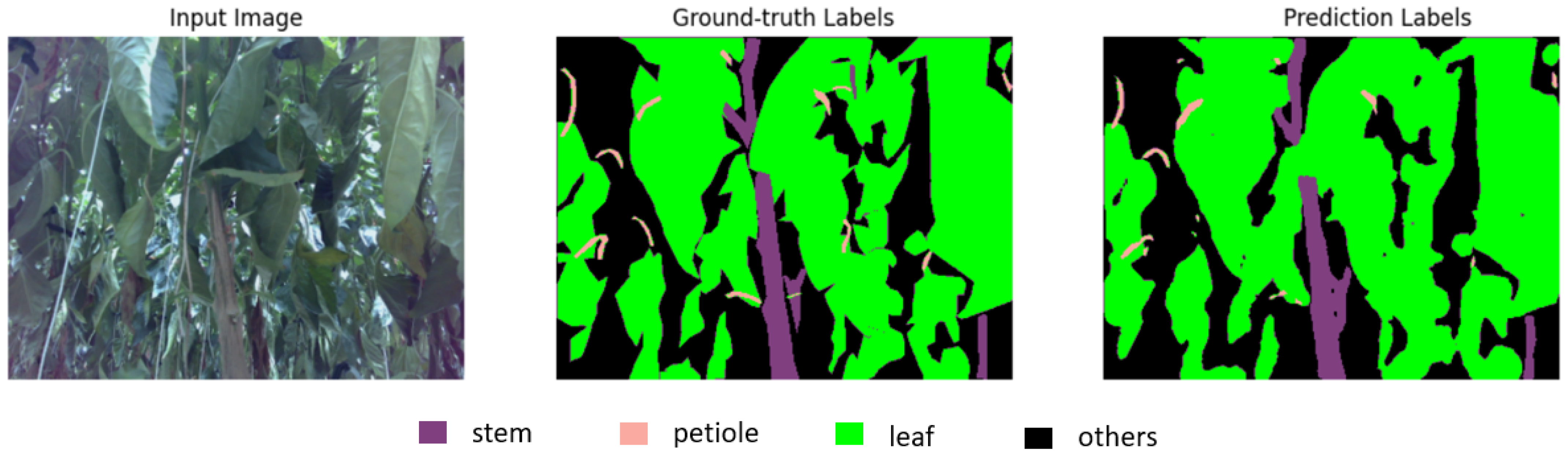
2.1. Semantic Segmentation Neural Network
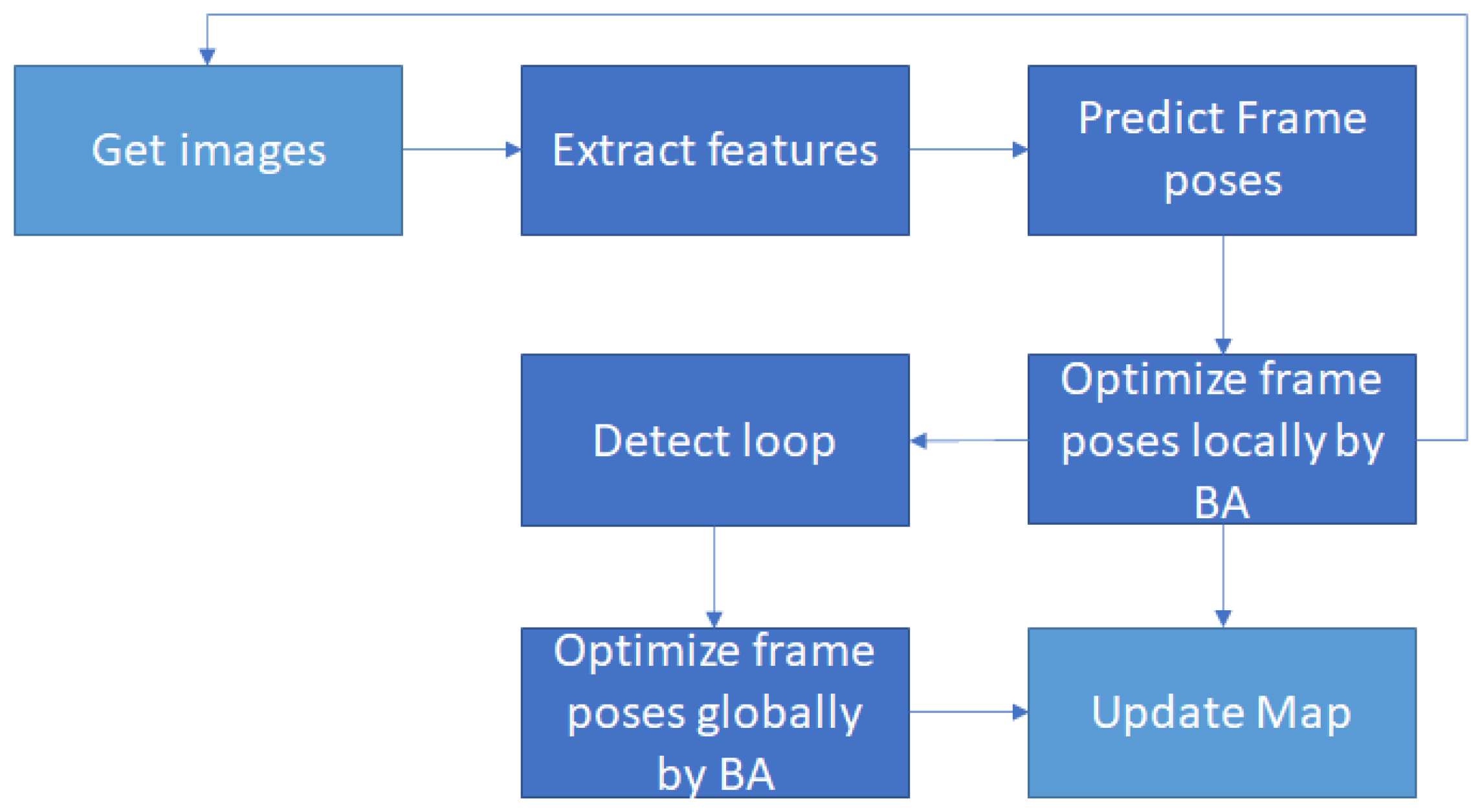
2.2. ORB-SLAM3
2.3. ICP Algorithm
3. Proposed System
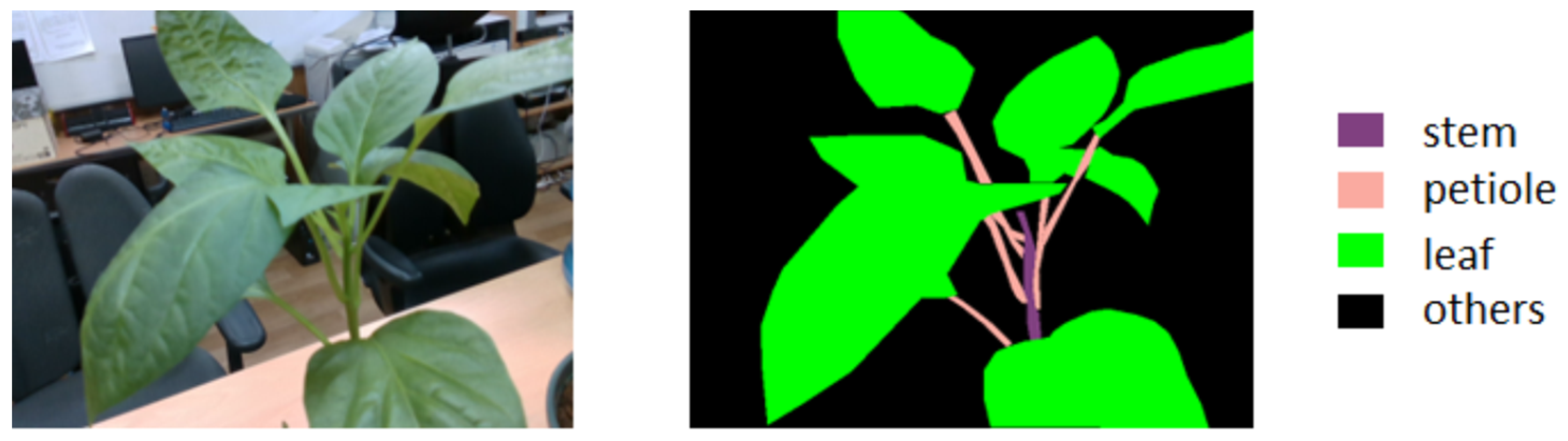
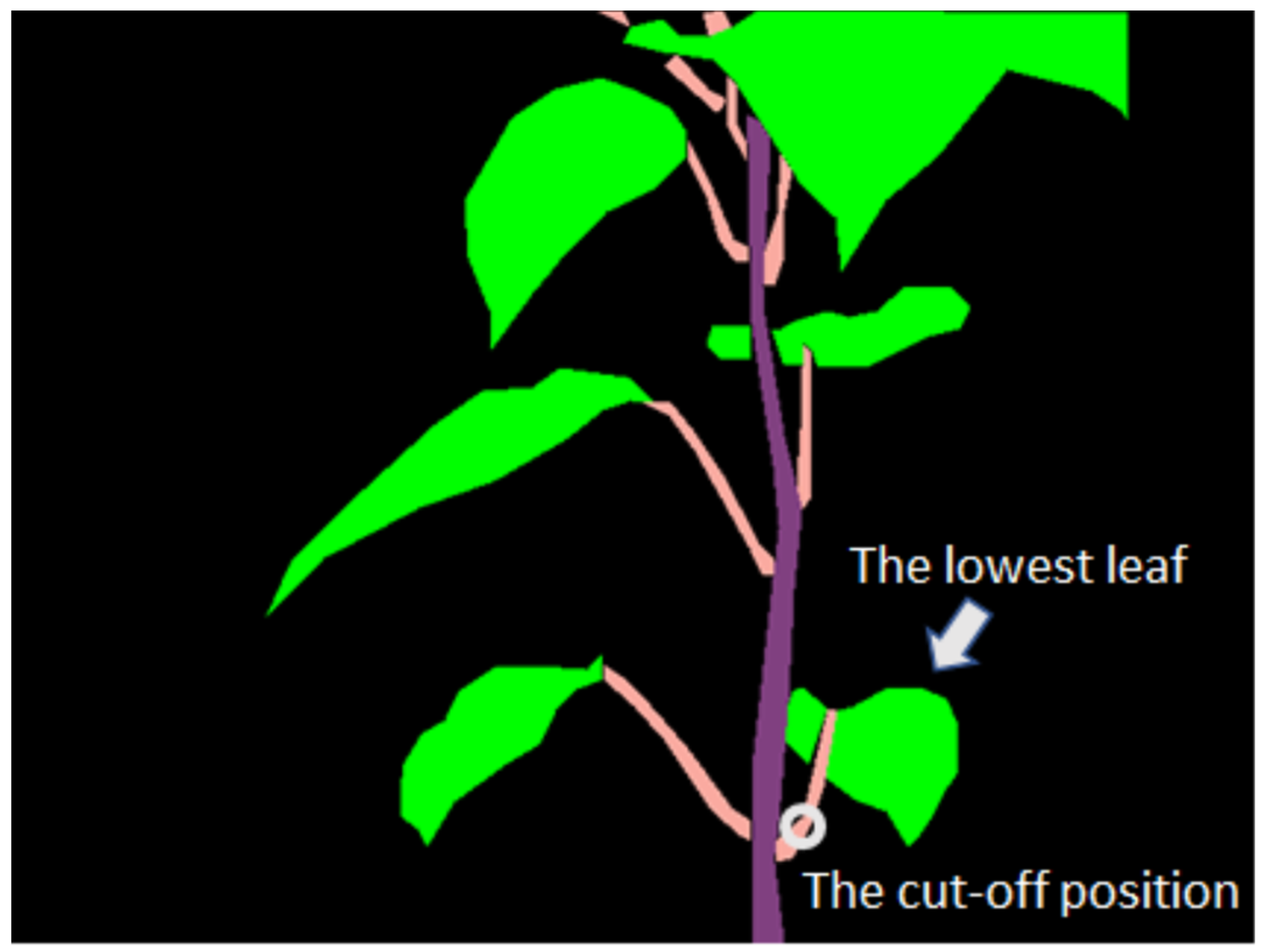
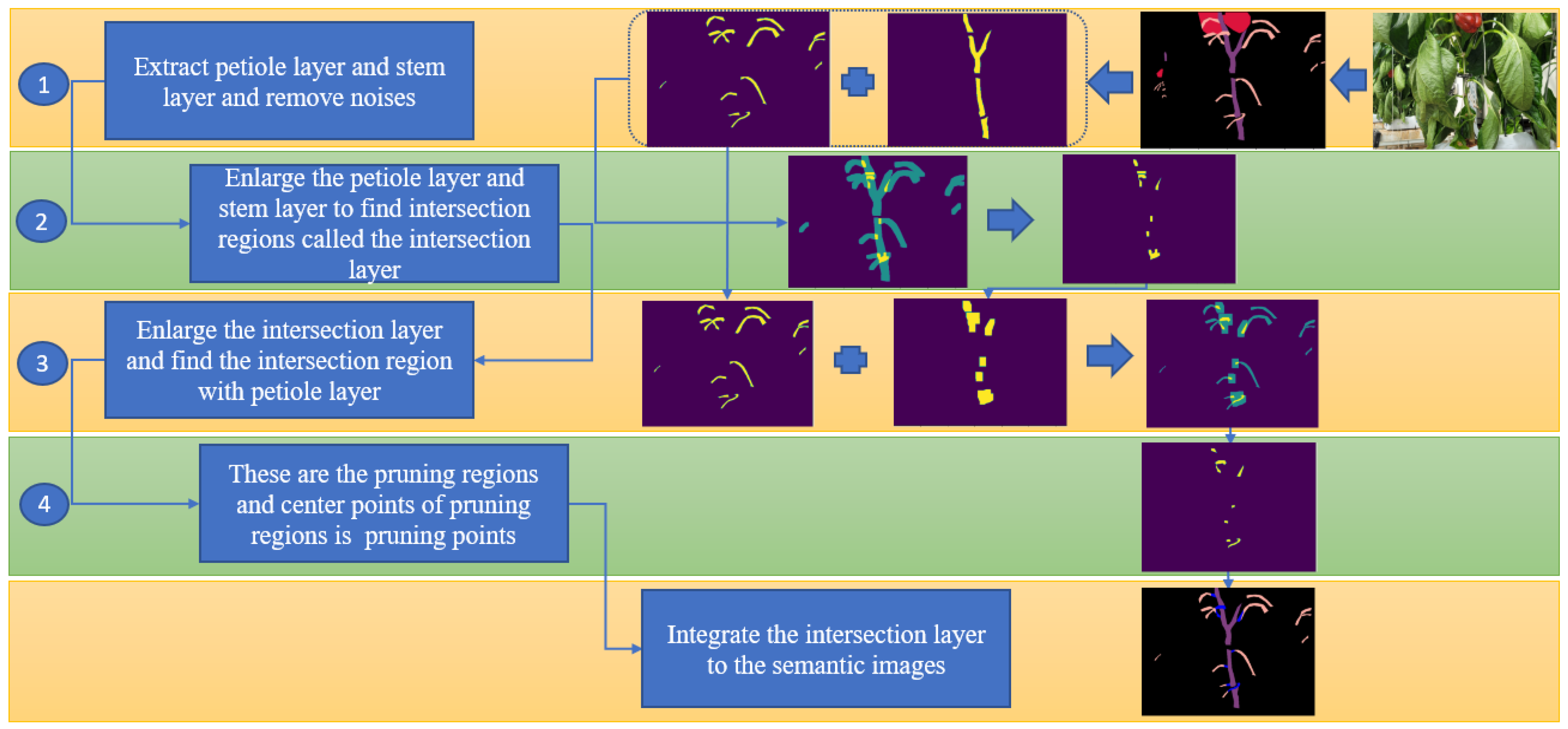
3.1. Detect Pruning Points and Pruning Regions in 2D Semantic Images
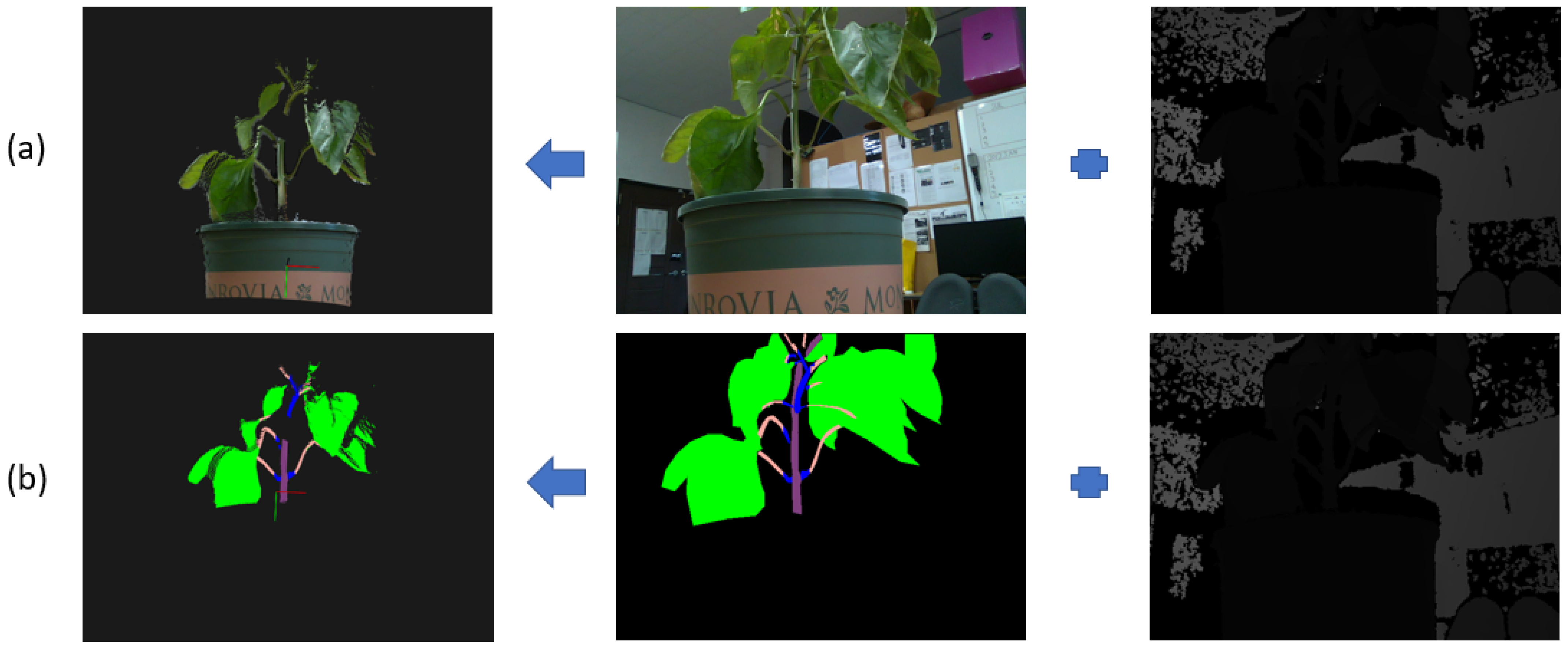
3.2. Create a 3D Semantic Point Cloud
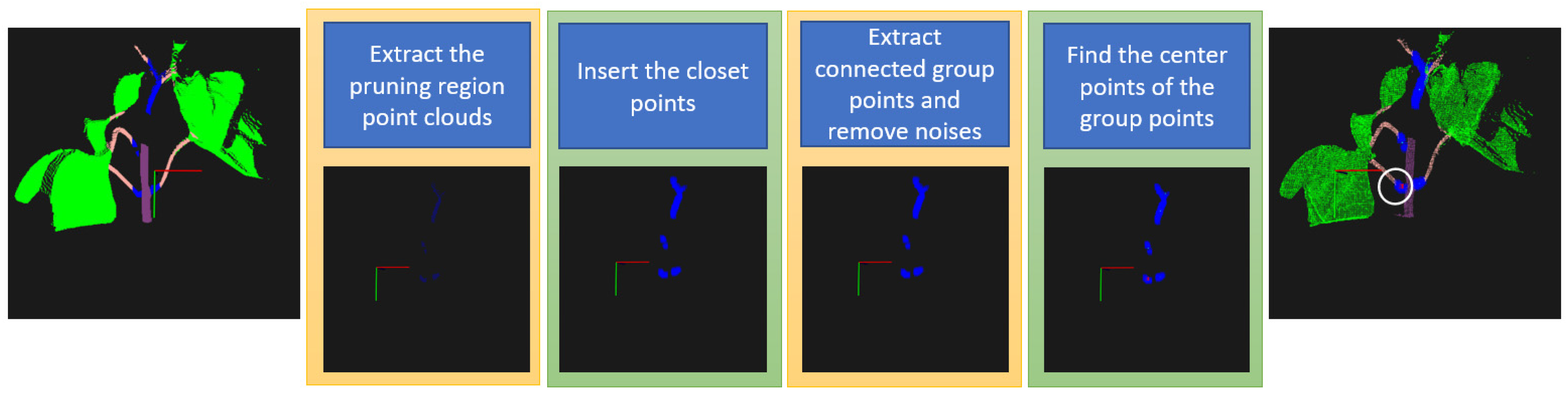
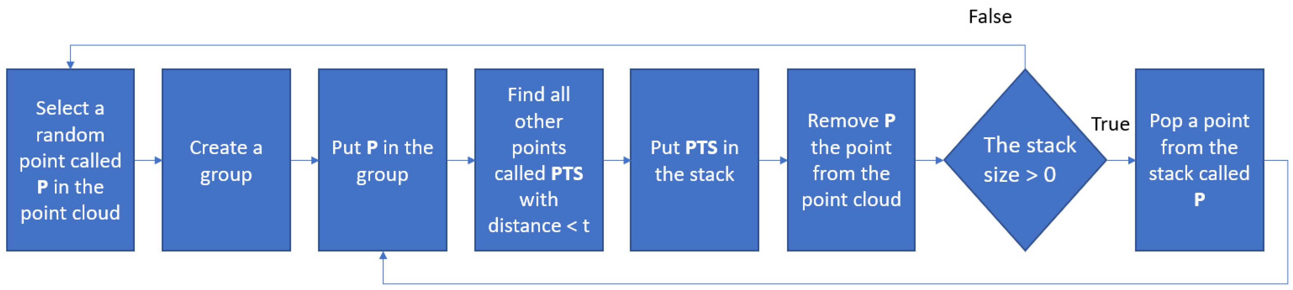
3.3. Detect Pruning Points in the 3D Semantic Point Cloud
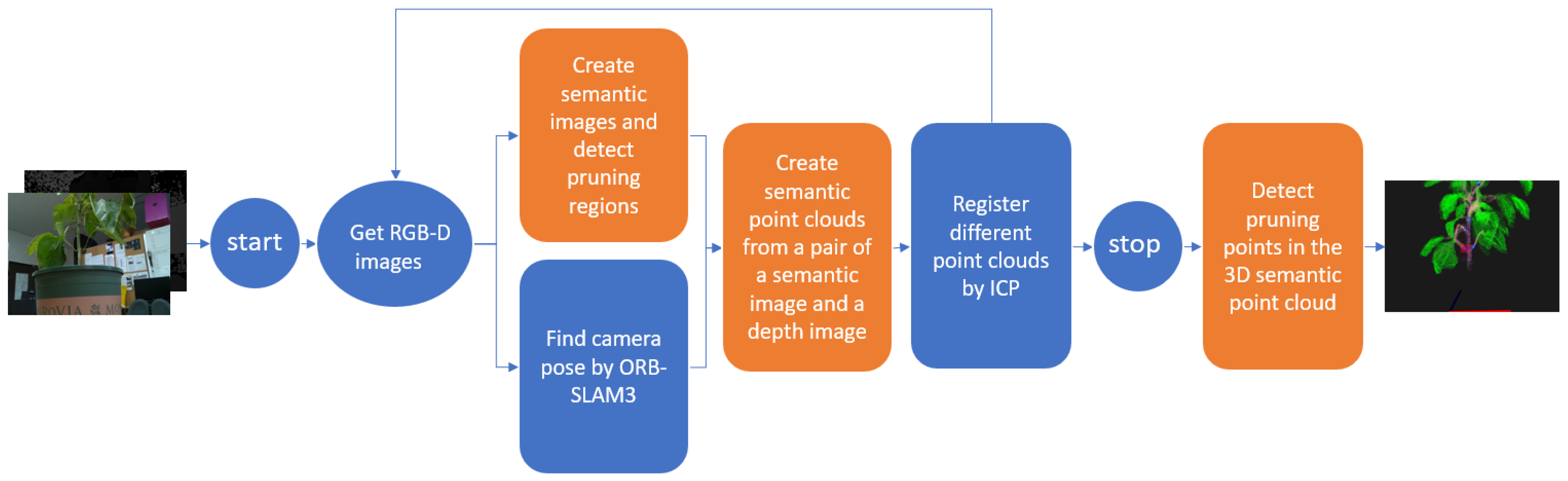
3.4. The Entire Pruning Points Detection System
4. Experiment and Results
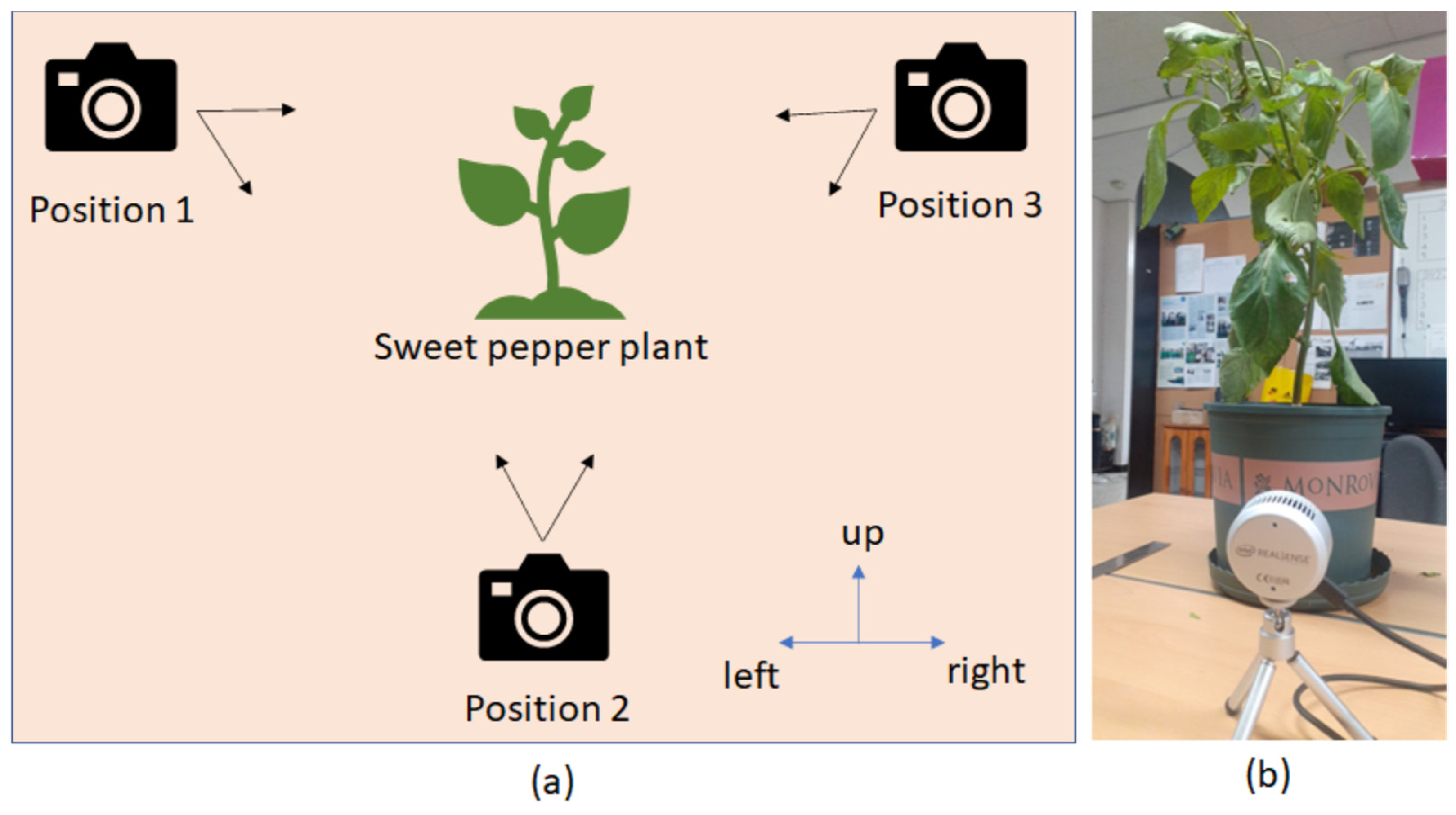
4.1. Experiment
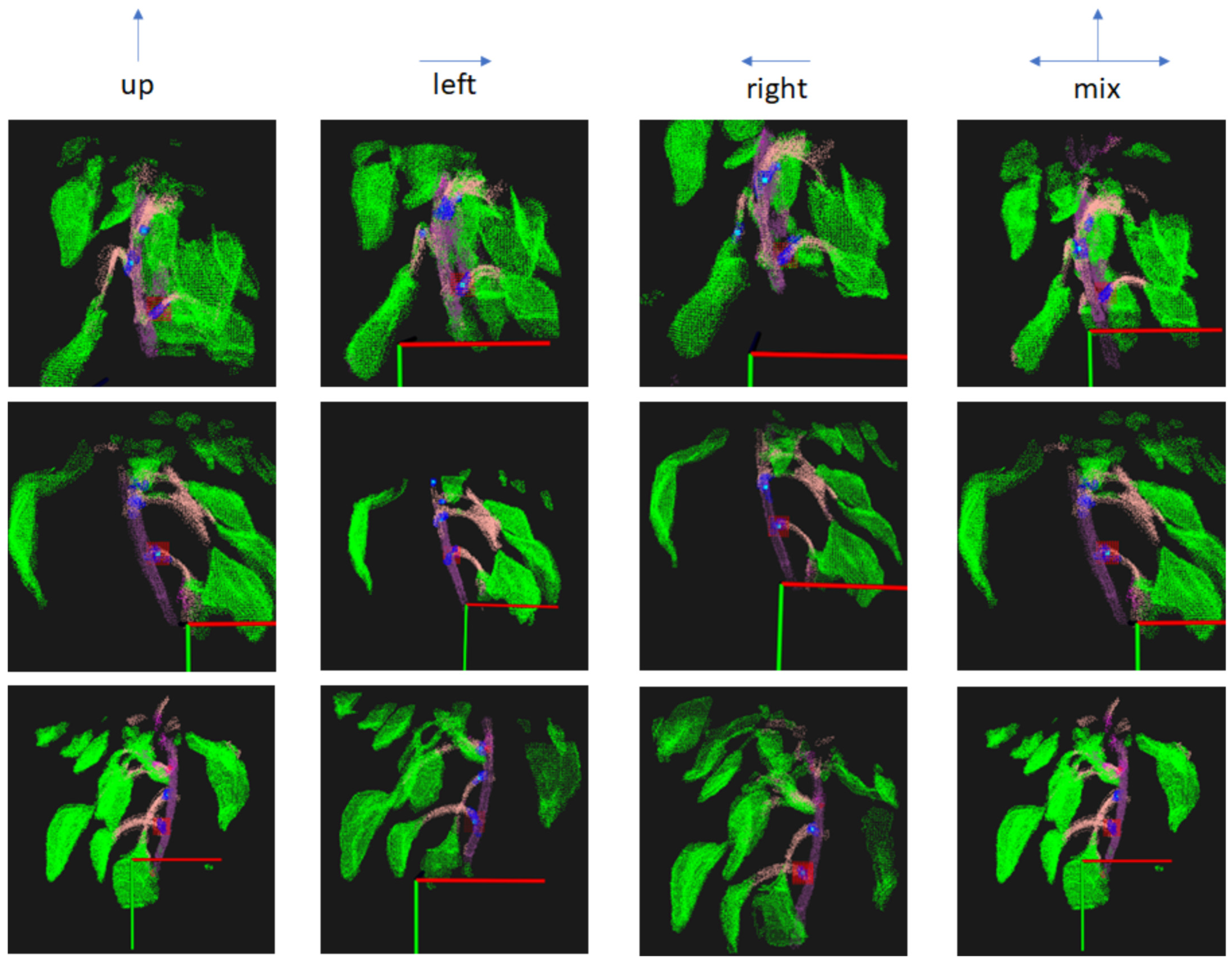
4.2. Results
4.3. Discussion
5. Conclusions
Author Contributions
Funding
Conflicts of Interest
References
- Malik, A.A.; Chattoo, M.A.; Sheemar, G.; Rashid, R. Growth, yield and fruit quality of sweet pepper hybrid SH-SP-5 (Capsicum annuum L.) as affected by integration of inorganic fertilizers and organic manures. J. Agric. Technol. 2011, 7, 1037–1048. Available online: http://ijat-aatsea.com/pdf/July_v7_n4_11/16 IJAT2011_Malik_R.pdf (accessed on 1 March 2018).
- Marín, A.; Ferreres, F.; Tomás-Barberán, F.A.; Gil, M.I. Characterization and quantitation of antioxidant constituents of sweet pepper (Capsicum annuum L.). J. Agric. Food Chem. 2004, 52, 3861–3869. [Google Scholar] [CrossRef]
- Sobczak, A.; Kowalczyk, K.; Gajc-Wolska, J.; Kowalczyk, W.; Niedzinska, M. Growth, yield and quality of sweet pepper fruits fertilized with polyphosphates in hydroponic cultivation with led lighting. Agronomy 2020, 10, 1560. [Google Scholar] [CrossRef]
- Alsadon, A.; Wahb-Allah, M.; Abdel-Razzak, H.; Ibrahim, A. Effects of pruning systems on growth, fruit yield and quality traits of three greenhouse-grown bell pepper (Capsicum annuum L.) cultivars. Aust. J. Crop Sci. 2013, 7, 1309–1316. [Google Scholar]
- Mussa, A.; Shinichi, K. Effect of planting space and shoot pruning on the occurrence of thrips, fruit yield and quality traits of sweet pepper (Capsicum annum L.) under greenhouse conditions. J. Entomol. Zool. Stud. 2019, 7, 787–792. [Google Scholar]
- Brenard, N.; Bosmans, L.; Leirs, H.; De Bruyn, L.; Sluydts, V.; Moerkens, R. Is leaf pruning the key factor to successful biological control of aphids in sweet pepper? Pest Manag. Sci. 2020, 76, 676–684. [Google Scholar] [CrossRef]
- Giang, T.T.H.; Khai, T.Q.; Im, D.; Ryoo, Y. Fast Detection of Tomato Sucker Using Semantic Segmentation Neural Networks Based on RGB-D Images. Sensors 2022, 22, 5140. [Google Scholar] [CrossRef]
- He, L.; Schupp, J. Sensing and automation in pruning of apple trees: A review. Agronomy 2018, 8, 211. [Google Scholar] [CrossRef]
- Lowe, D.G. Distinctive image features from scale-invariant keypoints. Int. J. Comput. Vis. 2004, 60, 91–110. [Google Scholar] [CrossRef]
- Viola, P.; Jones, M. Rapid object detection using a boosted cascade of simple features. In Proceedings of the IEEE Computer Society Conference on Computer Vision and Pattern Recognition, Kauai, HI, USA, 8–14 December 2001; Volume 1. [Google Scholar] [CrossRef]
- Maier, R.; Sturm, J.; Cremers, D. Submap-based bundle adjustment for 3D reconstruction from RGB-D data. In GCPR 2014: Pattern Recognition; Lecture Notes in Computer Science (including Subseries Lecture Notes in Artificial Intelligence and Lecture Notes in Bioinformatics); Springer: Berlin/Heidelberg, Germany, 2014; Volume 8753, pp. 54–65. [Google Scholar] [CrossRef]
- Rosten, E.; Drummond, T. Fusing Points and Lines for High Performance Real-Time Tracking; University of Cambridge: Cambridge, UK, 2005. [Google Scholar]
- Triggs, B.; McLauchlan, P.F.; Hartley, R.I.; Fitzgibbon, A.W. Bundle Adjustment—A Modern Synthesis. Zhonghua Wei Zhong Bing Ji Jiu Yi Xue 2000, 28, 298–372. [Google Scholar]
- Besl, P.J.; McKay, N.D. Method for registration of 3-D shapes. IEEE Trans. Pattern Anal. Mach. Intell. 1992, 14, 239–256. [Google Scholar] [CrossRef]
- Özyeşil, O.; Voroninski, V.; Basri, R.; Singer, A. A survey of structure from motion. Acta Numer. 2017, 26, 305–364. [Google Scholar] [CrossRef]
- Yu, F.; Gallup, D. 3D reconstruction from accidental motion. In Proceedings of the 2014 IEEE Conference on Computer Vision and Pattern Recognition, Columbus, OH, USA, 23–28 June 2014; pp. 3986–3993. [Google Scholar] [CrossRef]
- Henry, P.; Krainin, M.; Herbst, E.; Ren, X.; Fox, D. RGB-D mapping: Using Kinect-style depth cameras for dense 3D modeling of indoor environments. Int. J. Rob. Res. 2012, 31, 647–663. [Google Scholar] [CrossRef]
- Wang, K.; Zhang, G.; Bao, H. Robust 3D reconstruction with an RGB-D camera. IEEE Trans. Image Process. 2014, 23, 4893–4906. [Google Scholar] [CrossRef] [PubMed]
- Taketomi, T.; Uchiyama, H.; Ikeda, S. Visual SLAM algorithms: A survey from 2010 to 2016. IPSJ Trans. Comput. Vis. Appl. 2017, 9, 16. [Google Scholar] [CrossRef]
- Davison Real-time simultaneous localisation and mapping with a single camera. In Proceedings of the Ninth IEEE International Conference on Computer Vision, Nice, France, 13–16 October 2003; Volume 2, pp. 1403–1410.
- Davison, A.J.; Reid, I.D.; Molton, N.D.; Stasse, O. MonoSLAM: Real-Time Single Camera SLAM. IEEE Trans. Pattern Anal. Mach. Intell. 2007, 29, 1052–1067. [Google Scholar] [CrossRef]
- Newcombe, R.A.; Fitzgibbon, A.; Izadi, S.; Hilliges, O.; Molyneaux, D.; Kim, D.; Davison, A.J.; Kohi, P.; Shotton, J.; Hodges, S. KinectFusion: Real-time dense surface mapping and tracking. In Proceedings of the 2011 10th IEEE International Symposium on Mixed and Augmented Reality, Basel, Switzerland, 26–29 October 2011; pp. 127–136. [Google Scholar]
- Labbe, M.; Michaud, F. Online global loop closure detection for large-scale multi-session graph-based SLAM. In Proceedings of the 2014 IEEE/RSJ International Conference on Intelligent Robots and Systems, Chicago, IL, USA, 14–18 September 2014; pp. 2661–2666. [Google Scholar]
- Mur-Artal, R.; Montiel, J.M.M.; Tardos, J.D. ORB-SLAM: A Versatile and Accurate Monocular SLAM System. IEEE Trans. Robot. 2015, 31, 1147–1163. [Google Scholar] [CrossRef]
- Mur-Artal, R.; Tardos, J.D. ORB-SLAM2: An Open-Source SLAM System for Monocular, Stereo, and RGB-D Cameras. IEEE Trans. Robot. 2017, 33, 1255–1262. [Google Scholar] [CrossRef]
- Campos, C.; Elvira, R.; Rodriguez, J.J.G.; Montiel, J.M.M.; Tardos, J.D. ORB-SLAM3: An Accurate Open-Source Library for Visual, Visual-Inertial, and Multimap SLAM. IEEE Trans. Robot. 2021, 37, 1874–1890. [Google Scholar] [CrossRef]
- Botterill, T.; Paulin, S.; Green, R.; Williams, S.; Lin, J.; Saxton, V.; Mills, S.; Chen, X.; Corbett-Davies, S. A Robot System for Pruning Grape Vines. J. Field Robot. 2017, 34, 1100–1122. [Google Scholar] [CrossRef]
- Amatya, S.; Karkee, M.; Zhang, Q.; Whiting, M.D. Automated detection of branch shaking locations for robotic cherry harvesting using machine vision. Robotics 2017, 6, 31. [Google Scholar] [CrossRef]
- Rusu, R.B.; Cousins, S. 3D is here: Point Cloud Library (PCL). In Proceedings of the 2011 IEEE International Conference on Robotics and Automation, Shanghai, China, 9–13 May 2011; Volume 74, pp. 1–4. [Google Scholar]
- Quigley, M.; Gerkey, B.; Conley, K.; Faust, J.; Foote, T.; Leibs, J.; Berger, E.; Wheeler, R.; Ng, A. ROS: An open-source Robot Operating System. In Proceedings of the IECON 2015—41st Annual Conference of the IEEE Industrial Electronics Society, Yokohama, Japan, 9–12 November 2015. [Google Scholar] [CrossRef]


| Camera | Up (x, y, z) | Left (x, y, z) | Right (x, y, z) | Mix Path (x, y, z) | Average Difference (mm) |
|---|---|---|---|---|---|
| Position 1 | (15,−49,400) | (12,−45,401) | (22,−47,393) | (16,−48,401) | 4.19 |
| Position 2 | (−17,−75,388) | (−17,−76,391) | (−23,−75,388) | (−15,−80,394) | 6.15 |
| Position 3 | (50,−53,374) | (46,−54,374) | (50,−46,372) | (46,−51,376) | 4.01 |
Disclaimer/Publisher’s Note: The statements, opinions and data contained in all publications are solely those of the individual author(s) and contributor(s) and not of MDPI and/or the editor(s). MDPI and/or the editor(s) disclaim responsibility for any injury to people or property resulting from any ideas, methods, instructions or products referred to in the content. |
© 2023 by the authors. Licensee MDPI, Basel, Switzerland. This article is an open access article distributed under the terms and conditions of the Creative Commons Attribution (CC BY) license (https://creativecommons.org/licenses/by/4.0/).
Share and Cite
Giang, T.T.H.; Ryoo, Y.-J. Pruning Points Detection of Sweet Pepper Plants Using 3D Point Clouds and Semantic Segmentation Neural Network. Sensors 2023, 23, 4040. https://doi.org/10.3390/s23084040
Giang TTH, Ryoo Y-J. Pruning Points Detection of Sweet Pepper Plants Using 3D Point Clouds and Semantic Segmentation Neural Network. Sensors. 2023; 23(8):4040. https://doi.org/10.3390/s23084040
Chicago/Turabian StyleGiang, Truong Thi Huong, and Young-Jae Ryoo. 2023. "Pruning Points Detection of Sweet Pepper Plants Using 3D Point Clouds and Semantic Segmentation Neural Network" Sensors 23, no. 8: 4040. https://doi.org/10.3390/s23084040