Communication

The Performance Investigation of Smart Diagnosis for Bearings Using Mixed Chaotic Features with Fractional Order

1
Graduate Institute of Manufacturing Technology, National Taipei University of Technology, Taipei 10608, Taiwan
2
Institute for the Development and Quality, Macao 999078, China
3
Department of Electromechanical Engineering, Faculty of Science and Technology, University of Macau, Macao 999078, China
4
Master Program, Graduate Institute of Mechatronic Engineering, National Taipei University of Technology, Taipei 10608, Taiwan
5
Department of Mechanical Engineering, National Taipei University of Technology, Taipei 10608, Taiwan
6
Department of Computer Science and Engineering, National Taiwan Ocean University, Keelung City 202301, Taiwan
*
Author to whom correspondence should be addressed.
Sensors 2023, 23(8), 3801; https://doi.org/10.3390/s23083801
Submission received: 17 February 2023 / Revised: 30 March 2023 / Accepted: 2 April 2023 / Published: 7 April 2023

Abstract

:
This article presents a performance investigation of a fault detection approach for bearings using different chaotic features with fractional order, where the five different chaotic features and three combinations are clearly described, and the detection achievement is organized. In the architecture of the method, a fractional order chaotic system is first applied to produce a chaotic map of the original vibration signal in the chaotic domain, where small changes in the signal with different bearing statuses might be present; then, a 3D feature map can be obtained. Second, five different features, combination methods, and corresponding extraction functions are introduced. In the third action, the correlation functions of extension theory used to construct the classical domain and joint fields are applied to further define the ranges belonging to different bearing statuses. Finally, testing data are fed into the detection system to verify the performance. The experimental results show that the proposed different chaotic features perform well in the detection of bearings with 7 and 21 mil diameters, and an average accuracy rate of 94.4% was achieved in all cases.

1. Introduction

The popularization of precision manufacturing has led to increasingly demanding accuracy requirements in machining and manufacturing processes to ensure the normal operation of machines and to avoid damage to ball bearings without warning, which may cause operational failure of the machine or public security accidents. Therefore, it is necessary to detect whether the ball bearing is in a normal state or damaged. Many problems can be avoided if repairs are carried out in time before the bearing fails. Therefore, the purpose of this research is to develop methods and tools to further detect whether a bearing is damaged or not [1,2].
Several studies have shown that physical signals, such as stator currents [3], acoustic signals [4], and vibration signals [5], can be utilized for data exploration in the diagnosis of bearing failures. Among these signals, vibration signals are the most widely used choice. In real industrial production operations, machine vibration signals are considered to be one of the most effective and abundant physical signal sources for detecting bearing failure. Therefore, analyzing vibration signals has become critically important, with wavelet transform and Fourier analysis being two of the most common techniques for studying vibration signals.
Fast Fourier transform (FFT) [6,7] and short-time Fourier transform (STFT) [8] are popular Fourier-based methods for detecting fault conditions in bearings. Despite their good recognition capabilities, the fixed transformation windows of FFT and STFT result in inflexible resolution, making it challenging to achieve satisfactory resolution in both the time and frequency domains simultaneously. This factor makes it difficult to achieve satisfactory time and frequency domain resolutions simultaneously. Discrete Fourier analysis (DFA) [9] is another method that can clearly define the frequencies, locations, and ranges of fault states, but it performs poorly when the data present nonlinearity and time–frequency variations.
Wavelet analysis [10,11] is commonly used in data mining for various applications, such as Integrated Resonance-Based Sparse Signal Decomposition (RSSD) [12] and Wavelet Transform (WT) for fault diagnosis. However, practical applications remain challenging due to the wide range of frequency characteristics in bearings, which makes it difficult to select an effective mother wavelet for wavelet analysis. Additionally, physical sensors are often needed for wavelet transformations, leading to high costs and error rates. In other studies, empirical modal decomposition (EMD) has been used for data analysis and feature extraction, while the Hilbert transformation (HT) has been used for bearing failure diagnosis. However, in practice, the broad frequency spectrum of bearings results in the processing of intricate signals, making it challenging to determine the appropriate mother wavelet for wavelet analysis.
An alternative method for fault diagnosis was proposed by Yau et al. [13,14]. This method utilizes the theory of chaotic synchronous error dynamics and fractal theory. The characteristics of fractal theory have been further used to intercept error features, resulting in effective fault diagnosis, although this method requires additional time and professional experience to adjust the fraction order. Based on previous research achievements in applying chaotic systems, a smart detection system with a hierarchical structure of different features was proposed; this method simplifies the system structure and improves the efficiency of detection.
Li and Gu et al. [15,16,17] proposed Chaotic Mapping systems associated with a classification method extension theory. These systems are effective in identifying bearing fault states, but the processing of dynamic error signals requires extra time, leading to delayed diagnosis. To solve this disadvantage, this study applies fractional order chaotic synchronization to extract fewer signal characteristics of ball bearings and uses five different proposed feature extraction methods. This method allows the current state of a ball bearing system to be easily identified into four main fault states using a chaotic system.
Artificial Intelligence (AI) [18] algorithms have been a subject of discussion recently, particularly the use of Artificial Neural Networks (ANNs) and the breakthroughs in computing power that have made Deep Neural Networks (DNNs) [19,20] and Deep Learning (DL) [21] possible. These algorithms have demonstrated success in solving complex nonlinear classification problems between factor and dependent variables. However, the use of DL is limited by the need for large amounts of training data, complex learning structures, and high-intensity computing capabilities, making real-time monitoring of bearing status challenging. In contrast, Machine Learning (ML) can effectively solve linear classification and prediction problems with fewer training data and lower computational resources, making real-time monitoring of bearing states more feasible. However, ML has limitations in accurately solving complex nonlinear classification problems.
In the middle of the 20th century, thanks to the invention of computers, people were able to simulate weather phenomena and analyze the results through numerical simulations. According to “Deterministic Nonperiodic Flow” [22], edited by Edward Norton Lorenz, who sought to explain weather phenomena with a chaotic system, when a nonlinear system of differential equations has particular parameters, the system will show the properties of chaos. Chaos theory has the following characteristics: 1. The system is extremely sensitive to initial conditions, and different initial values have wildly different results; 2. The system is non-periodic in the long term; and 3. The system is deterministic. Thus, when the initial value is determined, we can predict its behavior. The aforementioned three properties of chaotic systems have the ability to change the characteristics of the original signal. The processed signal then undergoes the feature extraction technique proposed in this paper, which can facilitate signal analysis. Two application fields for this method will be discussed. First, because the system is extremely sensitive to initial conditions and does not converge on a single point, the chaotic system offers good performance in signal enlargement. Second, the properties of aperiodic long-term and deterministic behavior are extended using “Circuit Implementation of Synchronized Chaos with Applications to Communications” [23], edited by Kevin M. Cuomo and Alan V. Oppenheim. The spectrum of the chaotic system is wide enough to be applied in signal encryption [24]. We can use this phenomenon to produce chaotic mapping for the analysis, as the spectra of the signals have no limits.
After feature extraction, we choose extension theory as our identification method. Compared to other identification methods, extension theory does not require tedious parameter setting or a significant amount of calculations. These factors save not only computational resources but also computing time [13]. Compared to classical mathematical sets and fuzzy sets, extension sets have a wider area that can describe the degree of belonging. That is, extension sets can describe the degree of belonging in more detail. Taking fuzzy sets [25,26] and extension sets [27] as examples, the former only define the degree of belonging from 0 to 1, while the extension theory extends this to −∞ to +∞. Expanding the degree of belonging can offer a more detailed description, which has the potential to decrease classification errors. For this reason, we choose extension theory for this study. To summarize, we apply a method that combines a fractional order Chen–Lee chaotic system and extension theory to offer a shorter detection time and greater diagnosis rate. Finally, we present five feature extraction methods that have relatively high correct rates.
After the diagnostic procedure is determined, we will explain how to combine vibration signals with chaotic systems, feature extraction, and extension theory. The original vibration signal is a one-dimensional signal that is delayed and fed into the Chen–Lee chaotic system (x, y, z) in three dimensions as a preprocessing step. Then, the five proposed feature formulas are applied to the x, y, and z vectors, which is known as feature extraction. Finally, the diagnostic value calculated from feature extraction serves as a reference to classify and assess the accuracy of the input signal as either a normal state, ball fault, inner race fault, or outer race fault using extension theory.
The organization of this paper is described as follows. In Section 2, we discuss how to obtain the data source and perform data preprocessing. In Section 3, we present the advantages of using chaotic systems, explain how to process chaotic mapping, and demonstrate a phase diagram under various loading and failure states. In Section 4, inspired by the phase diagram, we propose five different feature extraction methods and apply them using the five formulae. In Section 5, we introduce extension theory and define the classic domain and joint field. In Section 6 and Section 7, we present the classification results and summarize the diagnosis conclusions.

2. Data Processing

2.1. Data Resource

The data used for simulation were obtained from Case Western Reserve University Bearing Data Center of the United States [28], which provides ball bearing test data for normal and faulty bearings. The test stand, depicted in Figure 1, is composed of a 2 hp motor on the left, a torque transducer/encoder in the center, and a dynamometer on the right. The motor shaft is supported by the test bearings, each subjected to a single point of failure (SPOF) using electro-discharge machining (EDM) with diameters of 7, 14, 21, 28, and 40 mils, as specified in the fault specifications, which also indicate fault depths of 0.011 inches. The defective bearings were reinstalled into the test motor. Then, we recorded vibration data for motor loads with different levels of horsepower. Finally, data were collected for normal bearings, single-point drive ends, and fan end defects. Then, we saved the results in MATLAB format. The test specifications are shown in Table 1. The fan end was the last section of the data resource and had a lower sampling rate; only the normal bearing and the SPOF drive end were used. Four states were provided on the inner raceway, rolling element (i.e., ball), outer raceway, and normal types.

2.2. Data Processing

Data were collected at 12,000 samples/second and 48,000 samples/second for the drive-end bearing experiments. As a result, the lengths of the data may be different.
For the simulation, we chose a sampling frequency of 48 k for the drive-end bearing experiments. However, the data length of 0 HP was different from that of other HPs. The length of the former was 240,000 samples and that of the latter was 480,000 samples. The 0 to 48,000th samples were not taken into consideration because the motor start-up caused one second transient state.
Additionally, data for SPOF with 0.014 inch on the inner race for 0 HP and 1 HP needed to be extended in order to obtain the same data length as other types of faults. After processing, the data were separated into two parts. One part was used for data training, and the other was used to verify the results shown in Table 2.

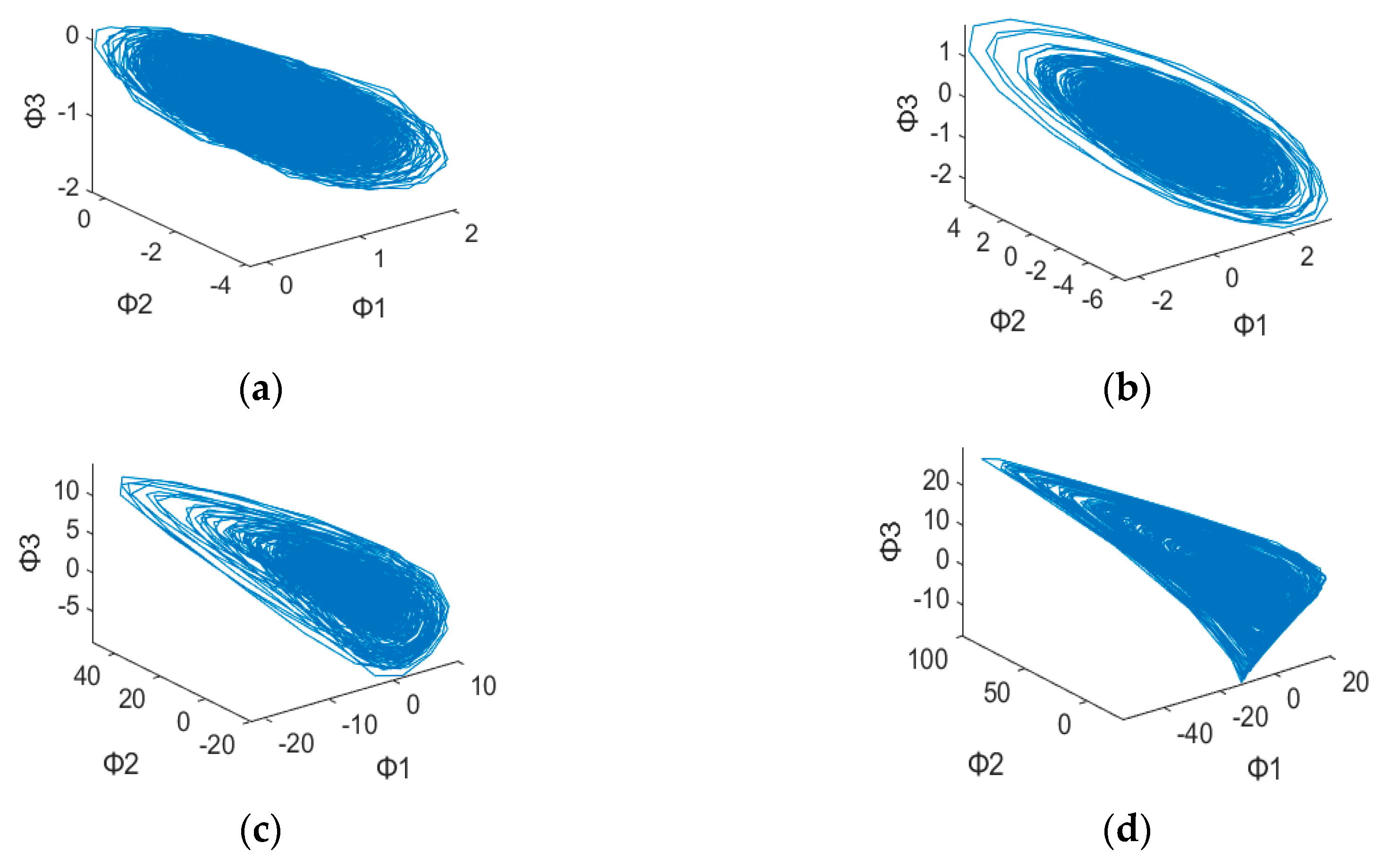
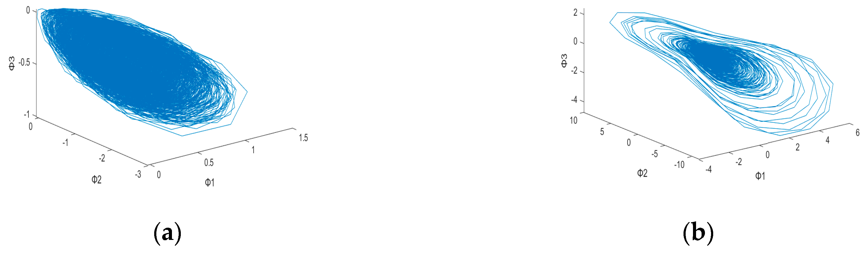
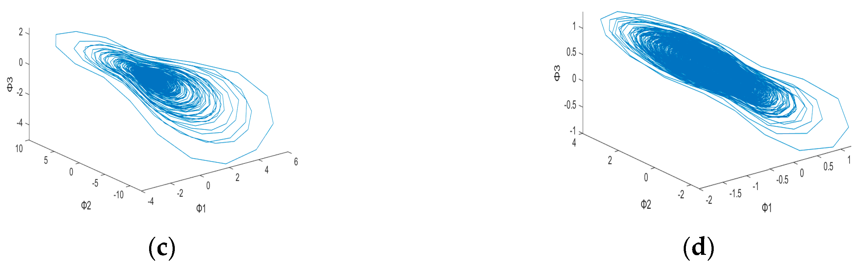
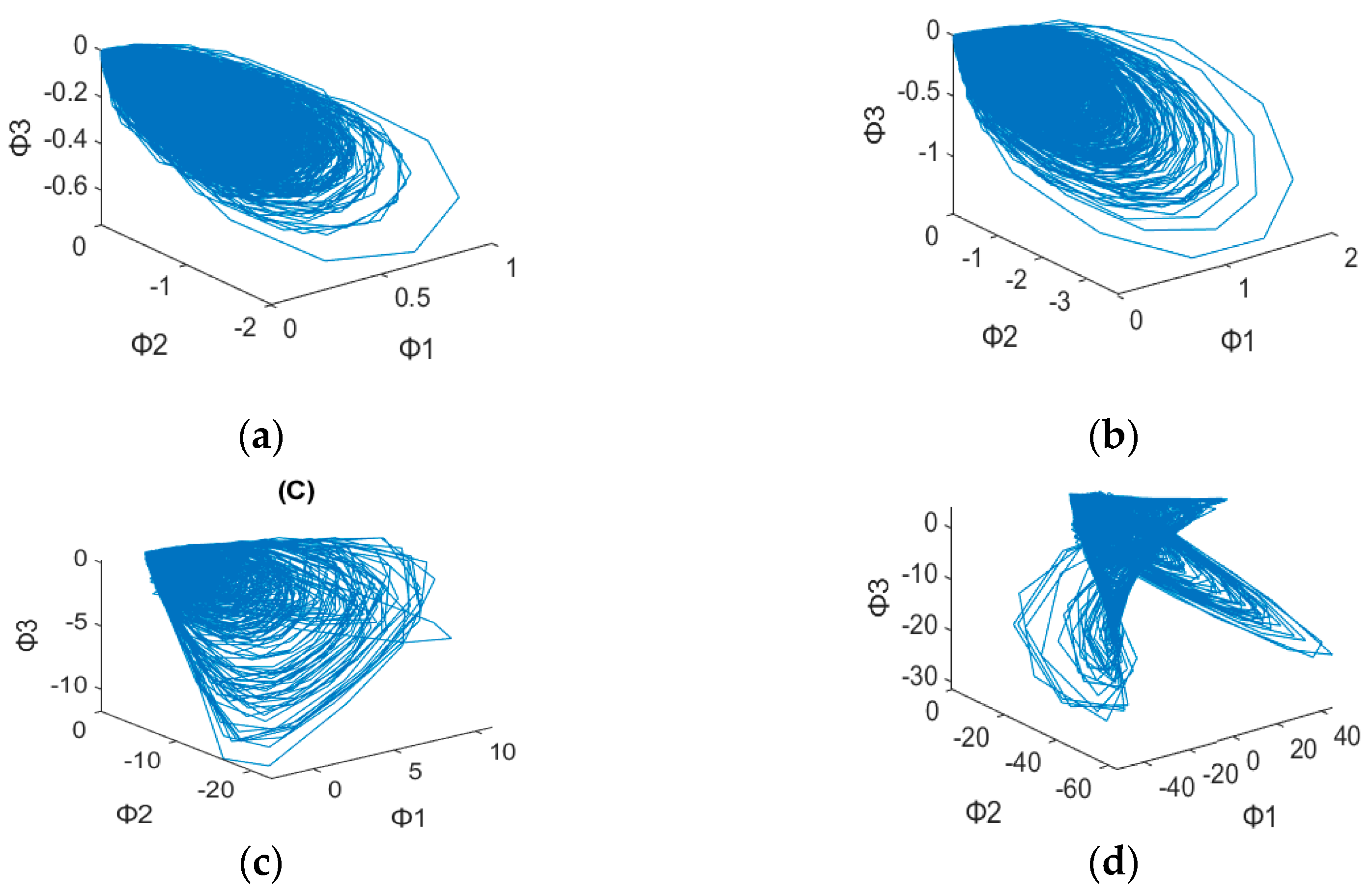
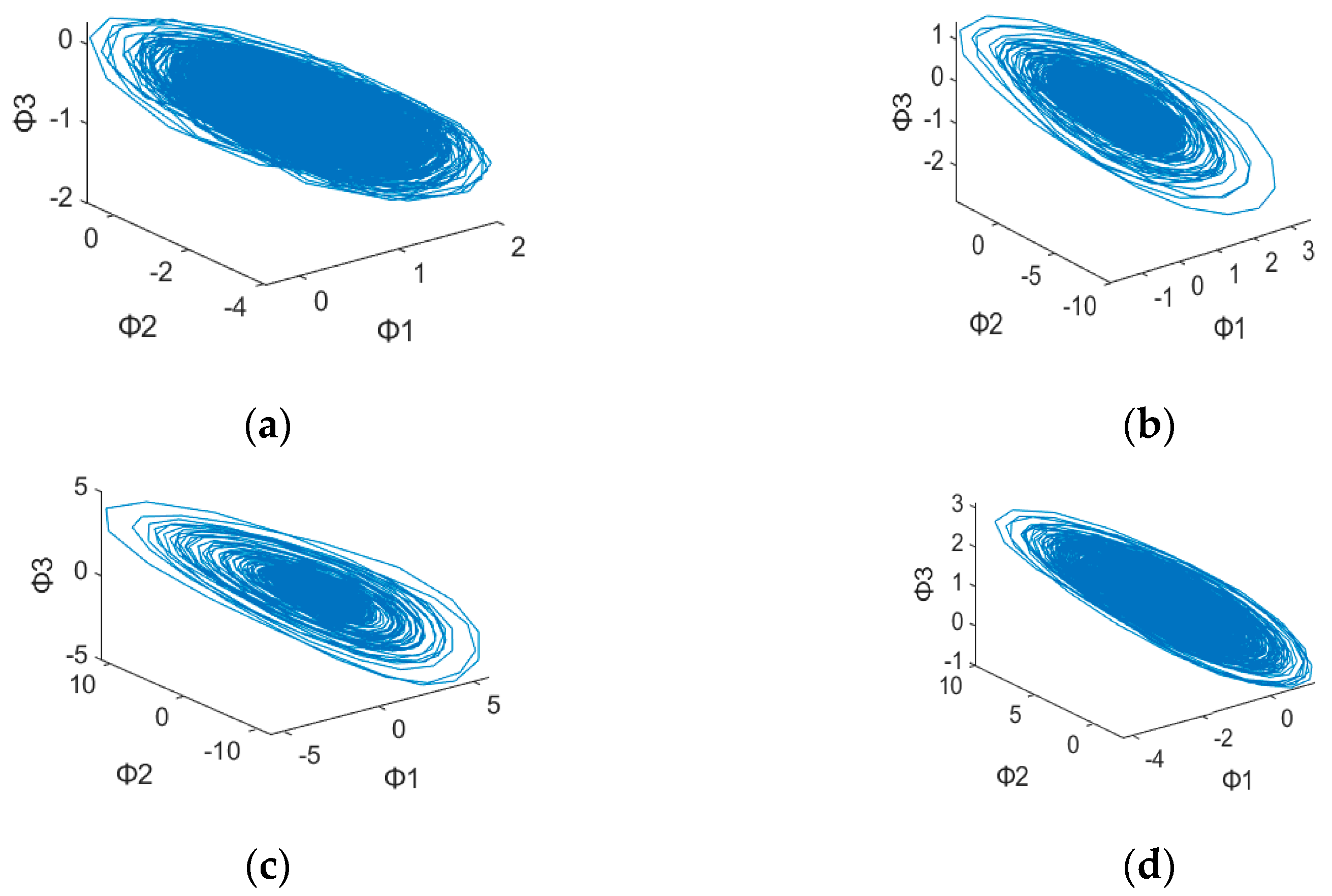
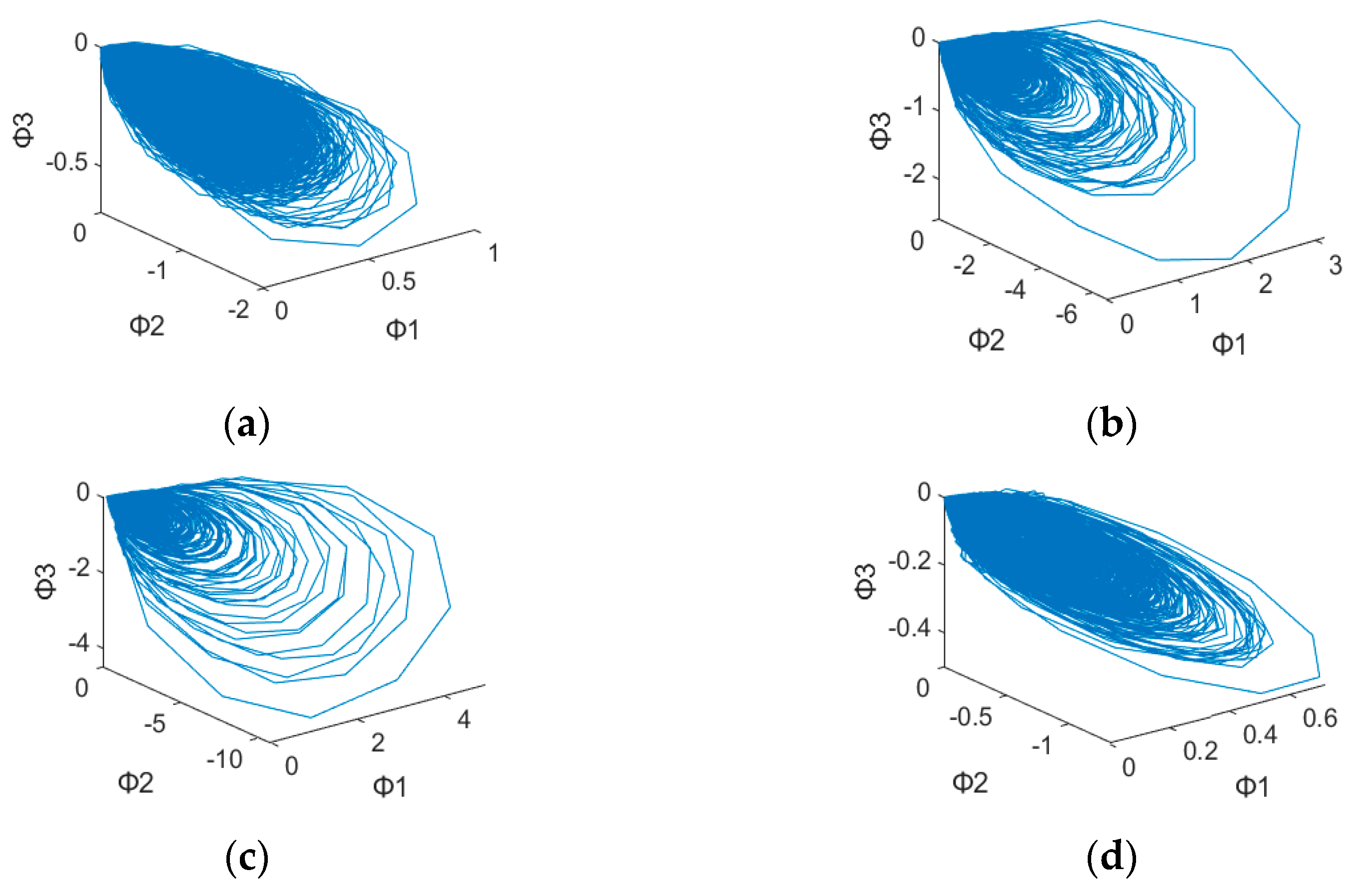
3. Chaotic Master–Slave System

3.1. Chaos Theory

The chaotic phenomenon results from the fact that objects continue replicating the state of motion in previous stages with some certain rules, which leads to unpredictable random effects. Therefore, a chaotic system is often used to discuss the behaviors that cannot be explained in dynamic systems with a single data relationship but can be predicted by a comprehensive data relationship. The chaotic system has some notable properties. First, the motion trajectory of the system is extremely sensitive to the initial value. Additionally, the chaotic system is a nonlinear system with randomness, indicating that the system has some potential principles that govern the system’s evolution, which can be predicted in a certain category and regarded as an important factor affecting the operation of the system. In this study, the above properties are used to identify the ball bearings in different states.

3.2. Chaotic Mapping

As Figure 2 shows, the ball bearing data are first preprocessed and transformed from one- to three-dimensional forms. Next, the data are entered into the chaotic mapping system, including a drive system xi, yi, zi and a response system xo, yo, zo, where xi, yi, zi are the coordinates of a fixed point and xo, yo, zo are the three-dimensional data of the ball bearing. Both systems are calculated by the Chen–Lee chaotic equations [29], represented as Equations (1) and (2).
x i = y i z i + a x i y i = x i z i + b y i z i = 1 3 x i y i + c z i
x o = y o z o + a x o + u 1 y o = x o z o + b y o + u 2 z o = 1 3 x o y o + c z o + u 3 .
Here, the response is subtracted from the driving system to form a set of dynamic errors, that is, e1, e2, e3. By using the fractional order derivatives of Grünwald–Letnikov [14], as in (3), an extra variable α can be obtained, and the new dynamic errors Φ1, Φ2, Φ3 are entered into the extension theory to identify different states of the ball bearing system.
D e α e m Γ m + 1 Γ m + 1 α e m α
After plotting the 3D dynamic error phase diagram with different values of α, the potential features maps are illustrated in Figure 3, Figure 4, Figure 5, Figure 6, Figure 7 and Figure 8 with α = 0, 0.3 and 0.6, which is also listed in Table 3. For α = 0, in Figure 3a,b, these are similar in both numerical range and shape, while Figure 3c,d have similar shapes, making them difficult to differentiate. Figure 6 has a significant overlap in the range of all four fault states, and the graphs and distribution densities are also similar, making analysis difficult. Both graph parameters are α = 0, so they are not ideal. For α = 0.6, Figure 5 and Figure 8 also have wide numerical ranges, but the distribution densities are very close to the origin, so they are also not suitable for use with parameters that are α = 0.6. Finally, For α = 0.3, in Figure 4b,c, these have similar shapes and ranges, but there is enough difference in the numerical range of Figure 4a,d to allow for classification. In Figure 7, there is a significant difference in the numerical distribution range, allowing for classification. According to the analysis mentioned above, an α value of 0.3 is decided, which is more suitable for diagnosis of bearing status.

4. Feature Extraction—Five Feature Extraction Methods for Performance Investigation
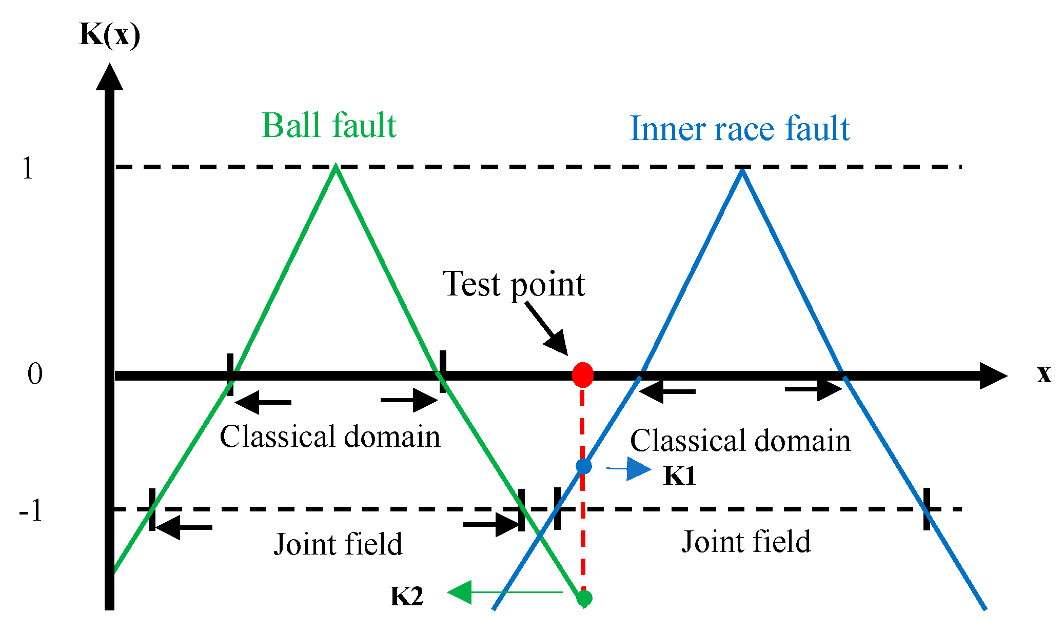
In order to identify the four different conditions of the ball bearing system, we must perform feature extraction. Feature extraction is a process used to simplify the initial data that allows data to be allocated to a more manageable group to facilitate learning and maintain data integrity. Sometimes, feature extraction can even offer a more complete interpretation of the initial data. The following are the five feature extraction methods used in this article:
Φ x Φ x m a x 2 + Φ y Φ y m a x 2
Φ x m a x / Φ x m i n
Φ x m a x Φ x m i n × Φ y m a x Φ y m i n
Φ x a v e 2 + Φ y a v e 2
Φ y Φ y a v e 2
After using Euclid’s distance between 2D dynamic errors and their maxima, the first method takes the maximum values as the characteristics. From the observations of the 2D phase diagram, we found that the graphs exhibit a ribbon distribution with different sizes. Therefore, the maximum values of x and y are deducted from the test points, and the Euclidean distance is taken to make the result close to the long side of the distribution. Then, we take the maximum value as the eigenvalue.
The second method uses only the x direction of dynamic errors, which is the ratio of maximum and minimum value. There are obvious differences between the maximum and minimum values of the four states in the x and y directions when observing the size of the 2D phase diagram. The difference in the x direction is more obvious, so we take the ratio of the maximum and minimum values in the x direction as one of the methods.
In the third method, we subtract the minimum values from the dynamic errors in the x and y directions and then multiply those values. According to the 2D phase diagram, the area of each graphic is different. It is suitable to use this property to identify the vibration signals. Since the area of the graphic is too difficult to calculate, we use the area of the rectangle, which represents the maximum and minimum area of the graphic.
Next, we use Euclid’s distance between the average point and origin of the 2D dynamic errors. Each average point of the vibration signals is separated in the 2D phase diagram, so the distribution of these points is useful for identification. We then calculate the value of Euclid’s distance between the average point and origin and use it as one of the characteristics for this study.
The last method is almost identical to the first but uses only the y direction, rather than 2D dynamic errors. The range of distribution for the characteristic values is known as the classical domain, which is included in the joint field. By observing the 2D phase diagram, the value of Φ2 under different error states is shown to be quite different. Therefore, the feature extraction method in method 5 mainly focuses on Φ2. We extract the maximum value of the distance between the Φ2 value of each point and the average value of Φ2 as the feature value and apply this method to this study.

5. Extension Theory

Generally, extension theory [30,31,32,33] is a method that helps to determine how related an object is to the feature by using an extension set and correlation function. Figure 9 presents a schematic of an extension set and correlation function. Briefly speaking, Figure 9 illustrates two triangles with different colors, and the horizontal and vertical axes represent the eigenvalues and correlation function, respectively. Additionally, assume that the green and blue triangles represent the correlation functions of the ball fault and inner race fault, respectively. Next, we compare K1 and K2, which represent the values of the correlation function shown in Figure 9, to determine which fault state the test point belongs to. Here, the test point is closer to the inner race fault, so the value of the correlation function is larger, i.e., K1 > K2. Thus, we classify this test point as the inner race fault. Eventually, by applying extension theory, we can compare the magnitude of each correlation function to determine which error state an observation belongs to.

6. Experimental Results

We conducted the multiple steps of this research using MATLAB. There are five main steps for feature extraction and testing.
  • Use pre-processed training and testing data to generate dynamic errors in the Chen–Lee chaotic mapping system.
  • Calculate the characteristics of dynamic errors based on the variety of the methods of feature extraction.
  • Set the classical domain and joint field by continuously training the characteristics.
  • Calculate the correlation functions of the different testing conditions with the testing characteristics, classical domain, and joint field in extension theory.
  • Compare the values of the correlation functions to determine the testing data (i.e., the vibration signal of the normal state, the ball fault state, the inner race fault state, and the outer race fault state).
In this research, we use five methods for feature extraction and three sets, each of which is handled by two methods. The weight of each method in the sets is 0.5. Table 4, Table 5, Table 6 and Table 7 show the classical domain and joint field of the second sets using different HP and 0.007 in SPOF diameters. In the table, the “X” symbol represents the third method, and the “Y” symbol represents the fourth method.
For the testing results, the accuracy of 0, 1, 2, and 3 HP is expressed in Table 8, Table 9, Table 10 and Table 11, respectively. The average accuracy is the average of the normal state, ball fault state, inner race fault state, and outer race fault state accuracy for the same SPOF and the same HP. This value represents the accuracy under a particular condition. In Table 12, the total average accuracy refers to the average accuracy in all conditions.
As shown in Table 12, the highest average accuracy in feature extraction was achieved by the second set. For feature extraction, this set used Euclid’s distance of the average area of a rectangle, determined by the maximum and minimum values in the 2D dynamic error phase diagram as characteristics. These two characteristics represent, respectively, the position and area information of the graphics. When a difficult condition, such as the 0.014 in SPOF diameter testing data, needs to be determined, the second set offers better effects because it provides the two different properties of dynamic errors.

7. Conclusions

This study focused on the effects of different feature extraction methods in the diagnosis of ball bearing vibration signals. After generating dynamic errors with the chaotic system, we assessed five feature extraction methods to calculate the classical domains and joint fields and then tested the accuracy of identification with extension theory under different conditions. According to the results, to obtain the highest accuracy ratio, it is necessary to analyze the properties of the dynamic errors in the phase diagram and to determine the appropriate characteristics.
Five feature extraction methods were proposed in this study, of which two were chosen as the basis for Methods 1 to 3. Method 1 used Equations (4) and (5), Method 2 used Equations (6) and (7), and Method 3 used Equations (7) and (8) as the two features X and Y for extension theory classification. The accuracy obtained from experiments using these three methods is presented in Table 8, Table 9, Table 10, Table 11 and Table 12, with Table 12 displaying the average accuracy of the three methods. The accuracy rates for Method 1, Method 2, and Method 3 were found to be 87.8%, 94.4%, and 84.8%, respectively. After comparing the results, we determined that Method 2 achieved the best and most stable classification results among the three methods. This paper also proposed a preprocessing step that utilizes a chaotic mapping system. Five different feature extraction equations were then used to develop three methods that utilized the two main features of X and Y. Finally, extension theory was employed for classification. Ultimately, our results show that the properties of feature extraction are the key factor needed to find the most accurate method for determining the ball bearing vibration signal. In the future, we will use the architecture in this study to develop improved methods for feature extraction with improved accuracy.

Author Contributions

Conceptualization, S.-Y.L., L.-M.T. and S.-C.C.; formal analysis, S.-Y.L., W.-L.T., C.-W.H., L.-Y.C. and Y.-X.X.; funding acquisition, L.-M.T.; investigation, S.-Y.L., L.-M.T., S.-P.W., W.-L.T., C.-W.H., L.-Y.C., Y.-X.X. and S.-C.C.; methodology, S.-Y.L., L.-M.T., S.-P.W., W.-L.T., C.-W.H., L.-Y.C. and S.-C.C.; project administration, S.-Y.L., L.-M.T. and S.-C.C.; resources, L.-M.T.; software, S.-P.W., W.-L.T., C.-W.H. and L.-Y.C.; supervision, S.-Y.L., L.-M.T., S.-P.W. and S.-C.C.; validation, S.-Y.L., L.-M.T., W.-L.T., C.-W.H., L.-Y.C. and S.-C.C.; visualization, S.-Y.L., S.-P.W., W.-L.T. and S.-C.C.; writing—original draft, W.-L.T., C.-W.H., L.-Y.C. and Y.-X.X.; writing—review and editing, S.-Y.L., L.-M.T., S.-P.W., W.-L.T., C.-W.H., L.-Y.C., Y.-X.X. and S.-C.C. All authors have read and agreed to the published version of the manuscript.

Funding

This paper was supported in part by the Institute for the Development and Quality, Macau, Macao, supported in part by the University System of Taipei Joint Research Program with grant no. USTP-NTUT-NTOU-112-03, supported in part by the Ministry of Education with grant no. PEE1110056, supported in part by the National Science and Technology Council, Taiwan, under grant number NSTC 111-2221-E-019-068-MY3, and by the Fisheries Agency, Council of Agriculture, Taiwan, under grant number 112AS-6.1.1-FA-F4.

Institutional Review Board Statement

Not applicable.

Informed Consent Statement

Not applicable.

Data Availability Statement

No new data were created in this paper.

Acknowledgments

The contribution of the master’s student Shih-Ping Wu and the college students Wei-Lin Tsai, Chia-Wen Hu, Li-Yang Cheng, and Yu-Xuan Xu were equal; they are the first student authors and worked together under our supervision. We also deeply appreciate the significant support from the Institute for the Development and Quality, Macau, Macao, National Taipei University of Technology, Taiwan, National Taiwan Ocean University, Taiwan, and the Ministry of Education, Taiwan.

Conflicts of Interest

The authors declare no conflict of interest. The funders had no role in the design of this study; in the collection, analysis, or interpretation of data; in the writing of the manuscript; or in the decision to publish the results.

References

  1. Sun, F.; Wei, Z. Rolling Bearing Fault Diagnosis Based on Wavelet Packet and RBF Neural Network. In Proceedings of the 2007 Chinese Control Conference, CCC Chinese, Zhangjiajie, China, 26–31 July 2007; pp. 451–455. [Google Scholar]
  2. Banks, J.; Brooks, J.; Cairns, G.; Davis, G.; Stacy, P. On Devaney’s definition of chaos. In The American Mathematical Monthly; Mathematical Association of America: Washington, DC, USA, 1992; Volume 99, pp. 332–334. [Google Scholar]
  3. Shifat, T.A.; Hur, J.W. An effective stator fault diagnosis framework of BLDC motor based on vibration and current signals. IEEE Access 2020, 8, 106968–106981. [Google Scholar] [CrossRef]
  4. Glowacz, A.; Tadeusiewicz, R.; Legutko, S.; Caesarendra, W.; Irfan, M.; Liu, H.; Brumercik, F.; Gutten, M.; Sulowicz, M.; Daviu, J.A.A.; et al. Fault diagnosis of angle grinders and electric impact drills using acoustic signals. Appl. Acoust. 2021, 179, 108070. [Google Scholar] [CrossRef]
  5. Chen, H.Y.; Lee, C.H. Vibration signals analysis by explainable artificial intelligence (XAI) approach: Application on bearing faults diagnosis. IEEE Access 2020, 8, 134246–134256. [Google Scholar] [CrossRef]
  6. Strömbergsson, D.; Marklund, P.; Berglund, K.; Larsson, P.E. Bearing monitoring in the wind turbine drivetrain: A comparative study of the FFT and wavelet transforms. Wind. Energy 2020, 23, 1381–1393. [Google Scholar] [CrossRef] [Green Version]
  7. Zhang, Z.; Wang, Y.; Wang, K. Fault diagnosis and prognosis using wavelet packet decomposition, Fourier transform and artificial neural network. J. Intel. Manuf. 2013, 24, 1213–1227. [Google Scholar] [CrossRef]
  8. Li, L.; Cai, H.; Han, H.; Jiang, Q.; Ji, H. Adaptive short-time Fourier transform and synchrosqueezing transform for non-stationary signal separation. Signal Process. 2020, 166, 107231. [Google Scholar] [CrossRef]
  9. Zhang, N.; Li, Y.; Yang, X.; Zhang, J. Bearing Fault Diagnosis Based on BP Neural Network and Transfer Learning. J. Phys. Conf. Ser. 2021, 1881, 022084. [Google Scholar] [CrossRef]
  10. Guo, J.; Liu, X.; Li, S.; Wang, Z. Bearing intelligent fault diagnosis based on wavelet transform and convolutional neural network. Shock Vib. 2020, 2020, 6380486. [Google Scholar] [CrossRef]
  11. Song, Y.H.; Zeng, S.K.; Ma, J.M. A fault diagnosis method for roller bearing based on empirical wavelet transform decomposition with adaptive empirical mode segmentation. Measurement 2018, 117, 266–276. [Google Scholar] [CrossRef]
  12. Lu, Y.; Du, J.; Tao, X. Fault diagnosis of rolling bearing based on resonance-based sparse signal decomposition with optimal Q-factor. Meas. Control 2019, 52, 1111–1121. [Google Scholar] [CrossRef] [Green Version]
  13. Yau, H.T.; Wu, S.Y.; Chen, C.L.; Li, Y.C. Fractional-order chaotic self-synchronization-based tracking faults diagnosis of ball bearing systems. IEEE Trans. Ind. Electron. 2016, 63, 3824–3833. [Google Scholar] [CrossRef]
  14. Chen, H.C.; Yau, H.T.; Chen, P.Y. Chaos synchronization error technique-based defect pattern recognition for GIS through partial discharge signal analysis. Entropy 2014, 16, 4566–4582. [Google Scholar] [CrossRef] [Green Version]
  15. Li, S.Y.; Gu, K.R. A Smart Fault-detection Approach with Feature Production and Extraction Processes. Inf. Sci. 2020, 513, 553–564. [Google Scholar] [CrossRef]
  16. Li, S.Y.; Gu, K.R.; Chieh, H.S. A Chaotic System-based Signal Identification Technology: Fault-Diagnosis of Industrial Bearing System. Measurement 2021, 171, 108832. [Google Scholar] [CrossRef]
  17. Li, S.Y.; Lin, Y.C.; Tam, L.M. A smart detection technology for personal ECG monitoring via chaos-based data mapping strategy. Multimed. Tools Appl. 2021, 80, 6397–6412. [Google Scholar] [CrossRef]
  18. Hamadache, M.; Jung, J.H.; Park, J.; Youn, B.D. A comprehensive review of artificial intelligence-based approaches for rolling element bearing PHM: Shallow and deep learning. JMST Adv. 2019, 1, 125–151. [Google Scholar] [CrossRef] [Green Version]
  19. Pham, T.A.; Tran, V.Q.; Vu, H.L.T.; Ly, H.B. Design deep neural network architecture using a genetic algorithm for estimation of pile bearing capacity. PLoS ONE 2020, 15, e0243030. [Google Scholar] [CrossRef]
  20. Ding, H.; Yang, L.; Cheng, Z.; Yang, Z. A remaining useful life prediction method for bearing based on deep neural networks. Measurement 2021, 172, 108878. [Google Scholar] [CrossRef]
  21. Zhang, S.; Zhang, S.; Wang, B.; Habetler, T.G. Deep learning algorithms for bearing fault diagnostics—A comprehensive review. IEEE Access 2020, 8, 29857–29881. [Google Scholar] [CrossRef]
  22. Lorenz, E.N. Deterministic Nonperiodic Flow. J. Atmos. Sci. 2020, 2, 130–141. [Google Scholar]
  23. Cuomo, K.M.; Oppenheim, A.V. Circuit Implementation of Synchronized Chaos with Applications to Communications. Phys. Rev. Lett. 1993, 71, 65–68. [Google Scholar] [CrossRef]
  24. Meng, X.; Ni, J.; Zhu, Y. Research on Vibration Signal Filtering Based on Wavelet Multi-resolution Analysis. In Proceedings of the 2010 International Conference on Artificial Intelligence and Computational Intelligence, Sanya, China, 23–24 October 2010; Volume 2, pp. 115–118. [Google Scholar]
  25. Chang, Y.C.; Chen, S.M.; Liau, C.J. Fuzzy Interpolative Rea soning for Sparse Fuzzy-Rule-Based Systems Based on the Areas of Fuzzy Sets. IEEE Trans. Fuzzy Syst. 2008, 16, 1285–1301. [Google Scholar] [CrossRef]
  26. Cai, W. Extension set, fuzzy set and classical set. In Proceedings of the 1st Congress of International Fuzzy System Association, Palma de Mallorca, Spain, 4–6 July 1985. [Google Scholar]
  27. Cai, W. Extension Set and Incompatible Problems. Sci. Explor. 1983, 3, 83–89. [Google Scholar]
  28. Case Western Reserve University Bearing Data Center. 2010. Available online: http://csegroups.case.edu/bearingdatacenter/page/welcomecase-western-reserve-university-bearing-data-center-websi (accessed on 19 August 2022).
  29. Chen, H.; Li, C. Anti-control of chaos in rigid body motion. Chaos Solitons Fractals 2004, 21, 957–965. [Google Scholar] [CrossRef]
  30. Hui, W.M. Application of extension theory to vibration fault diagnosis of generator sets. IEE Proc. Gener. Transm. Distrib. 2004, 151, 503–508. [Google Scholar]
  31. Wang, M.H.; Chen, H.C. Application of extension theoryto the fault diagnosis of power transformers. In Proceeding of the 22nd Symposium on Electrical Power Engineering, Kaohsiung, Taiwan, 21–22 November 2001; pp. 797–800. [Google Scholar]
  32. Huang, Y.P.; Chen, H.J. The extension-based fuzzy modelingmethod and its applications. In Proceedings of the 1999 IEEE Canadian Conference on Electrical and Computer Engineering, Edmonton, AB, Canada, 9–12 May 1999; pp. 977–982. [Google Scholar]
  33. Li, J.; Wang, S. Primary Research on Extension Control and System; International Academic Publishers: New York, NY, USA, 1991. [Google Scholar]
Figure 1. Ball bearing experiment platform.
Sensors 23 03801 g001
Figure 2. The procedure for converting original data into dynamic errors via chaotic mapping for ball bearing condition identification.
Sensors 23 03801 g002
Figure 3. 3D dynamic error phase diagram of a ball bearing under testing, with α = 0, HP = 0, and SPOF diameter = 0.007 in. (a) Normal state. (b) Ball fault. (c) Inner race fault. (d) Outer race fault.
Sensors 23 03801 g003
Figure 4. 3D dynamic error phase diagram of a ball bearing under testing, with α = 0.3, HP = 0, and SPOF diameter = 0.007 in. (a) Normal state. (b) Ball fault. (c) Inner race fault. (d) Outer race fault.
Sensors 23 03801 g004aSensors 23 03801 g004b
Figure 5. 3D dynamic error phase diagram of ball bearing under testing, with α = 0.6, HP = 0, and SPOF diameter = 0.007 in. (a) Normal state. (b) Ball fault. (c) Inner race fault. (d) Outer race fault.
Sensors 23 03801 g005
Figure 6. 3D dynamic error phase diagram of ball bearing under testing, with α = 0, HP = 0, and SPOF diameter = 0.014 in. (a) Normal state. (b) Ball fault. (c) Inner race fault. (d) Outer race fault.
Sensors 23 03801 g006
Figure 7. 3D dynamic error phase diagram of ball bearing under testing, with α = 0.3, HP = 0, and SPOF diameter = 0.014 in. (a) Normal state. (b) Ball fault. (c) Inner race fault. (d) Outer race fault.
Sensors 23 03801 g007
Figure 8. 3D dynamic error phase diagram of ball bearing under testing, with α = 0.6, HP = 0, and SPOF diameter = 0.014 in. (a) Normal state. (b) Ball fault. (c) Inner race fault. (d) Outer race fault.
Sensors 23 03801 g008
Figure 9. Illustration of a correlation function.
Sensors 23 03801 g009
Table 1. Data Information.
ParametersTypes
Sampling rate48 k (Hz)
Motor load0/1/2/3 (Hp)
SPOF diameter0.007/0.014/0.021 (in)
SPOF depth0.011 (in)
Type of faultNormal/Inner Race Fault/Ball Fault/Outer Race Fault
Table 2. Training Data and Testing Data.
Training DataTesting Data
Motor load 0 Hp with different diameters of faults48,000–144,000th144,001–240,000th
Motor load 1/2/3 Hp with different diameters of faults48,000–264,000th264,001–480,000th
Table 3. 3D Dynamic Error Phase Diagram of Ball Bearing Under Testing.
Figure\StateSPOFα
Figure 30.007 inα = 0
Figure 40.007 inα = 0.3
Figure 50.007 inα = 0.6
Figure 60.014 inα = 0
Figure 70.014 inα = 0.3
Figure 80.014 inα = 0.6
Table 4. Classical Domain and Joint Field When SPOF Diameter = 0.007 in, HP = 0.
StateClassical DomainJoint Field
NormalX <3.336 4.811>
Y <1.071 1.090>
X <2.968 5.179>
Y <1.066 1.095>
Ball faultX <1106 1464>
Y <1.204 1.275>
X <1017 1554>
Y <1.186 1.293>
Inner race faultX <16.69 30.97>
Y <1.028 1.062>
X <13.12 34.55>
Y <1.020 1.070>
Outer race faultX <7383 9604>
Y <1.574 1.649>
X <6828 10,158>
Y <1.555 1.669>
Table 5. Classical Domain and Joint Field When SPOF Diameter = 0.007 in, HP = 1.
StateClassical DomainJoint Field
NormalX <3.336 4.811>
Y <1.071 1.090>
X <2.968 5.179>
Y <1.066 1.095>
Ball faultX <1106 1464>
Y <1.204 1.275>
X <1017 1554>
Y <1.186 1.293>
Inner race faultX <16.69 30.97>
Y <1.028 1.062>
X <13.12 34.55>
Y <1.020 1.070>
Outer race faultX <7383 9604>
Y <1.574 1.649>
X <6828 10,158>
Y <1.555 1.669>
Table 6. Classical Domain and Joint Field When SPOF Diameter = 0.007 in, HP = 2.
StateClassical DomainJoint Field
NormalX <2.756 6.106>
Y <1.066 1.101>
X <1.919 6.944>
Y <1.058 1.109>
Ball faultX <222.0 287.0>
Y <1.277 1.330>
X <205.8 303.3>
Y <1.264 1.343>
Inner race faultX <13.50 24.10>
Y <1.125 1.184>
X <10.85 26.75>
Y <1.109 1.199>
Outer race faultX <4568 6023>
Y <1.598 1.690>
X <4204 6387>
Y <1.575 1.713>
Table 7. Classical Domain and Joint Field When SPOF Diameter = 0.007 in, HP = 3.
StateClassical DomainJoint Field
NormalX <3.000 4.538>
Y <1.059 1.116>
X <2.615 4.922>
Y <1.045 1.130>
Ball faultX <183.5 237.6>
Y <1.303 1.349>
X <170.0 251.1>
Y <1.291 1.361>
Inner race faultX <12.42 27.98>
Y <1.132 1.184>
X <8.531 31.87>
Y <1.118 1.197>
Outer race faultX <4976 6454>
Y <1.602 1.670>
X <4606 6824>
Y <1.585 1.687>
Table 8. Accuracy When HP = 0.
MethodMethod 1Method 2Method 3
SPOF Diameter
(10−3 in)
714217142171421
Normal (%)10010010010083.998.210080.292.4
Ball fault (%)100100100100100100100100100
Inner race fault (%)10059.910010088.410010065100
Outer race fault (%)1000100100100100100100100
Average (%)10064.910010093.199.610086.398.1
Table 9. Accuracy When HP = 1.
MethodMethod 1Method 2Method 3
SPOF Diameter
(10−3 in)
714217142171421
Normal (%)10010010010010010010090.9100
Ball fault (%)10089.990.410068.810010088.7100
Inner race fault (%)10091.984.210010010010091.1100
Outer race fault (%)10010010010071.410010092.7100
Average (%)10095.593.610085.110010090.8100
Table 10. Accuracy When HP = 2.
MethodMethod 1Method 2Method 3
SPOF Diameter
(10−3 in)
714217142171421
Normal (%)100100100100100100100100100
Ball fault (%)10010010010071.3100100100100
Inner race fault (%)100010010088.610010000
Outer race fault (%)100010010051.31001000100
Average (%)1005010010077.81001005075
Table 11. Accuracy When HP = 3.
MethodMethod 1Method 2Method 3
SPOF Diameter
(10−3 in)
714217142171421
Normal (%)10010010010087.68810076.385.7
Ball fault (%)10010010010098.5100100100100
Inner race fault (%)100010010069.798.710000
Outer race fault (%)100096.610068.21001006.4100
Average (%)1005099.11008196.610046.571.4
Table 12. Total Average Accuracy.
MethodMethod 1Method 2Method 3
Total
Average
Accuracy (%)
87.894.484.8
Disclaimer/Publisher’s Note: The statements, opinions and data contained in all publications are solely those of the individual author(s) and contributor(s) and not of MDPI and/or the editor(s). MDPI and/or the editor(s) disclaim responsibility for any injury to people or property resulting from any ideas, methods, instructions or products referred to in the content.

