Proactive Fault Prediction of Fog Devices Using LSTM-CRP Conceptual Framework for IoT Applications

Abstract
:1. Introduction
2. Literature Survey
- Self-healing: is defined as a system’s capacity to have a self-recovery mechanism for errors by employing particular fault recovery techniques on occasion procedures that involve tasks for monitoring.
- Pre-emptive migration: is described as a system’s capacity to transfer computation away from hazardous processing nodes in a proactive fashion.
- System rejuvenation: this is a procedure for regularly taking a system backup. Following every backup, the device is cleaned before the backup is restored, resulting in a refreshed state of the system.
- Load balancing: is employed to distribute the load on the processor and memory when it has reached its maximum limit. The workload of a CPU that has reached its maximum capacity is moved to a different CPU that has the processor and memory available.
- Checkpoint restart: this function periodically saves the states of a task’s execution. In the event of a failure, the job is restarted from the most recent state that has been saved as opposed to starting from scratch.
- Job migration: in the event of a resource failure, the job switches to another instance of a similar and appropriate resource.
- Replication: used to produce numerous copies of jobs and store copies in various places, such as the primary backup strategy, which places the primary replica on one machine and the copy of the backup on a different device.
3. Problem Definition
- Predictive Period: This period is a pre-defined period just before a failure. When an alert is given during this period there is enough time for the administrators to react and terms to be successful. The time the alert is given to the starting time of the failure is the specified time window W.
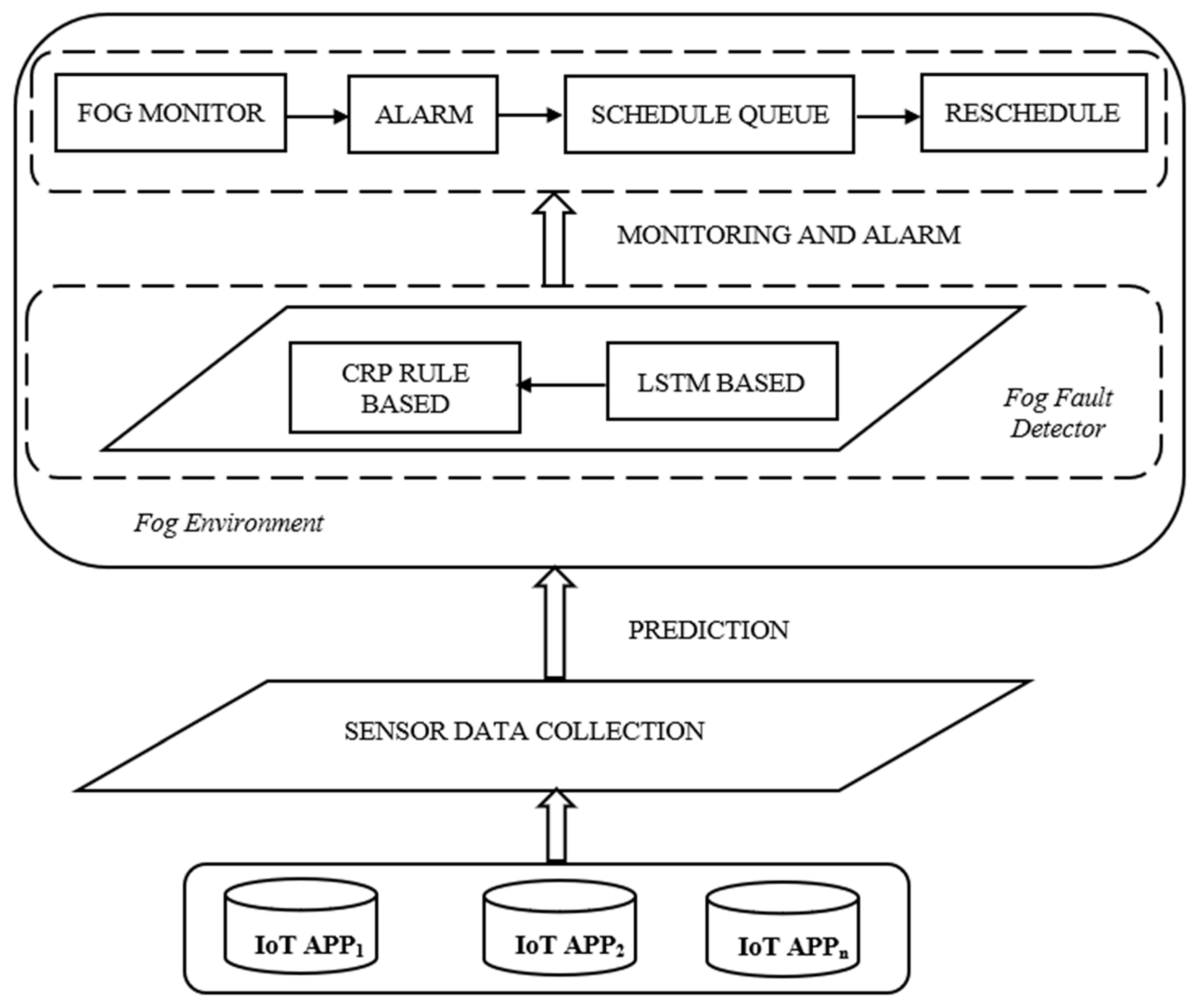
4. Proposed Methodology
4.1. Fault Detector
4.1.1. LSTM Fault Prediction Network
| Algorithm 1: Computation algorithm of LSTM Cell |
| Input: Output: Generating Algorithm: BEGIN |
| Initializations , , , , , , |
| while i < time_steps: do |
| Step 1: LSTM—Forget gate |
| Step 2: LSTM—Input gate |
| Step 3: LSTM—Output gate |
| end while END |
- Forget Gate: This gate, which is the first one in the LSTM cell, determines whether or not the data from the preceding stamp will be kept. The data from the current input state Jn and hidden state bn−1 are acquired, a function named sigmoid is applied to produce an output within 0 and 1, and then the cell state from the preceding timestamp is multiplied with the result. If the decisive number is 1, nothing is forgotten. However, if the decisive number is 0, everything is forgotten.
- Input Gate: A value within 0 and 1 is produced by applying another function of sigmoid to the current Jn and hidden bn−1 states in the input gate before the tanh function is used on it. The state of the cell is then modified to a different cell state after taking the vector input values and adding them stepwise.
- Output Gate: The information contained in the hidden state for the following cycle is determined by applying a third function of sigmoid to the current state, the preceding hidden state, and the recent state of the cell produced in the input gate. Point-by-point multiplication is performed on both outputs and chooses what data the subsequent cycle’s hidden state will contain. The hidden state is transmitted over to the following step together with the new state of the cell.
LSTM Fault Trainer
| Algorithm 2: LSTM Fault Trainer |
| Input: Total no. of fog devices-α Each fog device—β Resources of fog devices—{FN_C+S, FNA_C+S, FN_UD, FN_level, FN_pow} No. of features, fNum Function for Transformation-g(.)–{w1,w2} |
| Output: Running status of the device(fog status)—ψ |
| Generating Algorithm BEGIN G = [] lt = α [len (α) – 1] for each β in α while j < fNum m⟵m + pow (β [j] – lt[j], 2.0) j + 1 end while G.append(sqrt (m)) end for // Standardizing the values of G to [− 1, 1] G⟵std_normalize(G) while j < len (α) E[j]⟵g(j) j⟵ j + 1 end while E⟵std_normalize(E) while j < len(α) ψ [j]⟵w1* G[j] + w2* E[j] end while return ψ END |
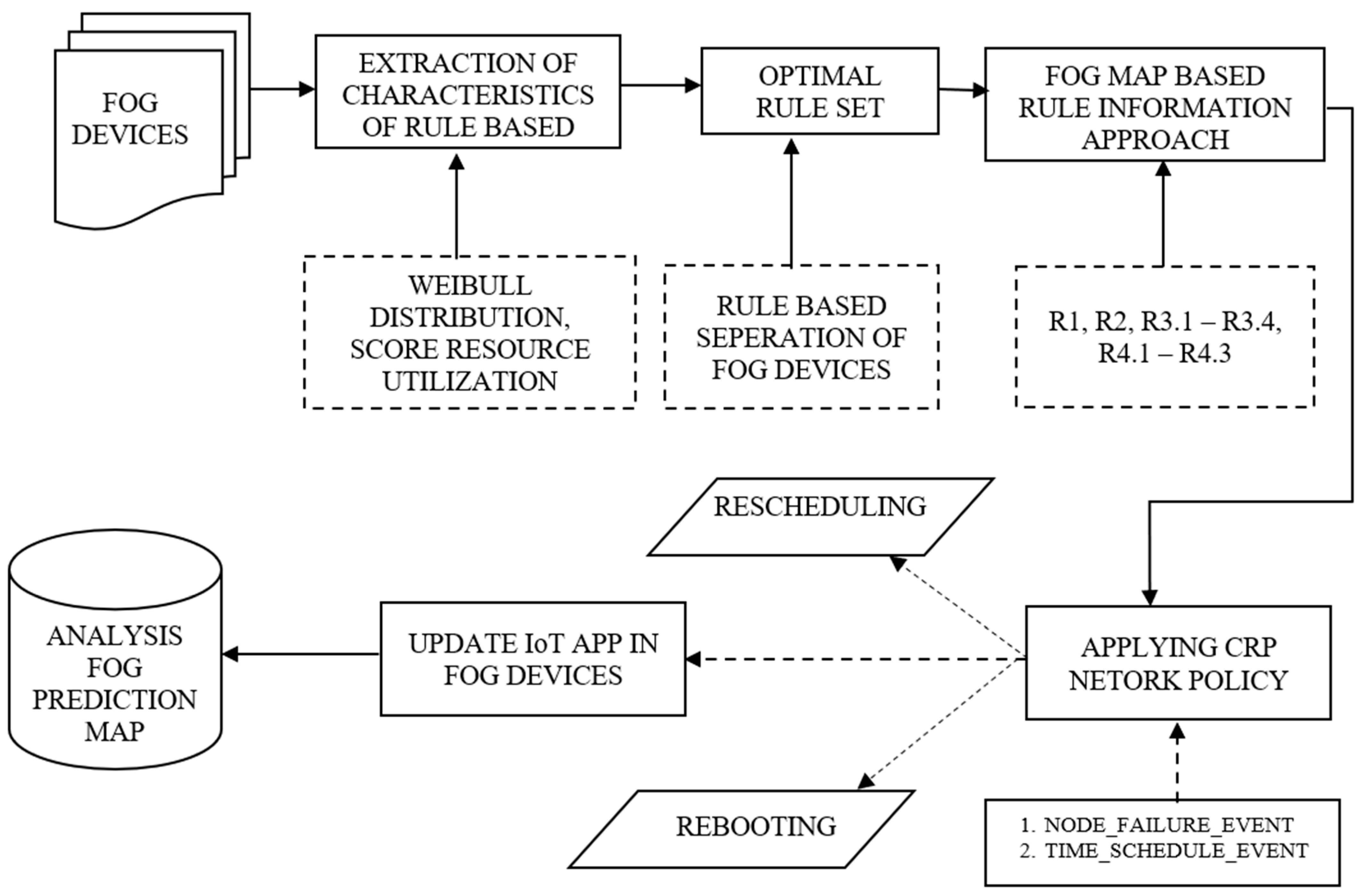
4.1.2. CRP Rule-Based Network Policy
- (a)
- We horizontally divide the resources of each fog device in the data set.
- (b)
- Each node consists of its scanned data subset that generates a set of resources.
- (c)
- The resources of each fog device are divided into r partitions that are different.
- (d)
- These r partitions of the nodes accumulate the score of the fog device and produce the final score, which determines the failure after comparing it with the minimum score.
- (e)
- From the observed outputs, the set of failed failure traces of fog nodes is generated.
Characteristics of Rule-Based Aspect Extraction Approach
Optimal Rule Set and its Robustness
- (a)
- Rule 1:
| R1 = R1(FNA_C+S) R1: if res(FNA_C+S v FN_UD v FN_pow v FN_level) < res(Y_C+S) →(−1,+1), {insufficient resources of CPU + RAM} |
- (b)
- Rule 2:
| R2 = R2(FNA_C+S, FN_UD, FN_pow, FN_level) R2: if res(FNA_C+S ᴧ FN_UD ᴧ FN_pow ᴧ FN_level) < res(Y_C+S) →(−2,+2), {FN_fault},{del(FN)} |
- (c)
- Rule 3:
| R3 = R3(FN_C+S) R3: if avail(FNA_C+S)! = res(Y_C+S) if avail(FNA_C+S) > res(Y_C+S) → = True {strong sufficient resources} if avail(score(FNA_C+S)) > 0 ᴧ avail(FN_level) >= 1 → avail(Y_C+S) {insufficient resources of CPU, RAM and level} if avail(ψ (FN_C)) < 0 ᴧ avail(ψ (FN_S)) > 0 ᴧ avail(FN_level) >= 1 -> (Y_C+S) {insufficient resources of CPU} (FN_C)) > 0 ᴧ avail(FN_level) >= 1 → (Y_C+S) then {insufficient resources of RAM} |
- (d)
- Rule 4:
| R4 = R4(FN_pow) R4: if res(FN_pow € (busy,idle) if ψ (FN_pow) > 0 ᴧ avail(ψ (FNA_C+S)) > 0 ᴧ avail(FN_level) >= 1 -> ψ (FN_pow) > ψ (IoT_pow) {sufficient resources} if ψ (FN_pow) < 0 ᴧ avail(ψ (FNA_C+S)) > 0 ᴧ avail(FN_level) >= 1 -> ψ (FN_pow) < ψ (IoT_pow) {insufficient resources} if ψ (pow_idle) < 0 -> ψ (fn_busypow) = ψ (IoT_power) {insufficient resources of power} |
CRP Rule-Based Algorithm Policy
| Algorithm 3: CRP Rule-Based Network Policy |
| Data_Structure: Fog_Node_List, a list of nodes that cater to IoT applications. Fog_Node_Pool_Schedule, a list of scheduled nodes waiting to service the IoT Applications Node_Pool_List, idle nodes list. In this list, the most recently failed nodes are moved to the top and they are set to the current time. In the meantime, move non-failed nodes, including those that are intentionally rejuvenated, to the end of the list. HPC_IoTApp_Running_List, HPC running IoT Applications in a list. HPC_IoTApp_Finished_List, HPC finished IoT Applications in a list |
| Output: Prediction of Failure |
| Assumptions: All of this data is extracted from the logger of the devices Fog_Node_failure_Event; Time_Schedule_Event; |
| Generating Algorithm: BEGIN while (RM_getevent(e_type) // Resource Manager identifies the failure event switch(e_type) case Fog_Node_Failure_Event: put FailureNode.uptime = CurrentTime; push(Fog_Node -> Node_Pool_List) pull(Fog_Node_Pool_Schedule) case Time_Schedule_Event: HPC_IoTApp_Running_List → request(res(Fog_Node)) for each Fog_Node in Fog_Node_List if ({R1 or R2 or R3 or R4} == True) Redirects(FogNode to Rescheduler) push(Fog_Node -> Node_Pool_List) push(HPC_IoTApp_Running_List -> Fog_Node_Pool_Schedule) Allocate avail(FNA_C+S) -> avail(x_C+S) Response.Redirect (FogNode); end if if ({R1 or R2 or R3 or R4} == False) if(!(Rescheduled)) reboot() elif(lowpriority) push(HPC_IoTApp_Running_List -> cloud) elif (new_rule) generate_new_rule(new_rule) end if end if for each IoTApp in HPC_IoTApp_Running_List if(IoTApp.ExecuteTime + IoTApp.StartTime > CurrentTime) put IoTApp.status = finished push( IoTApp -> HPC_IoTApp_Finished_List) push(Fog_Node -> Fog_Node_Pool_Schedule) end if end for end for end switch end while END |
| Algorithm 4: Generate new rules |
| Input: S is the list of training data C is the list of different classes |
| Output: R Rules are produced, R = []//initially an empty list. |
| Generating Algorithm generate new_rule() Begin if (C [R1,R2,R3,R4]) // the new failure class found does not belong to any of the rules. for every class C // for every new class found while(C != S) // while the class does not belong to training data create new_rule C R.append(new_rule) end while end for end if End |
4.2. Fault Monitor
5. Results and Discussion
5.1. Experimental Setup and Failure Modelling
5.2. Evaluation Metrics
- a.
- Minimum Delay
- b.
- Processing Time
- c.
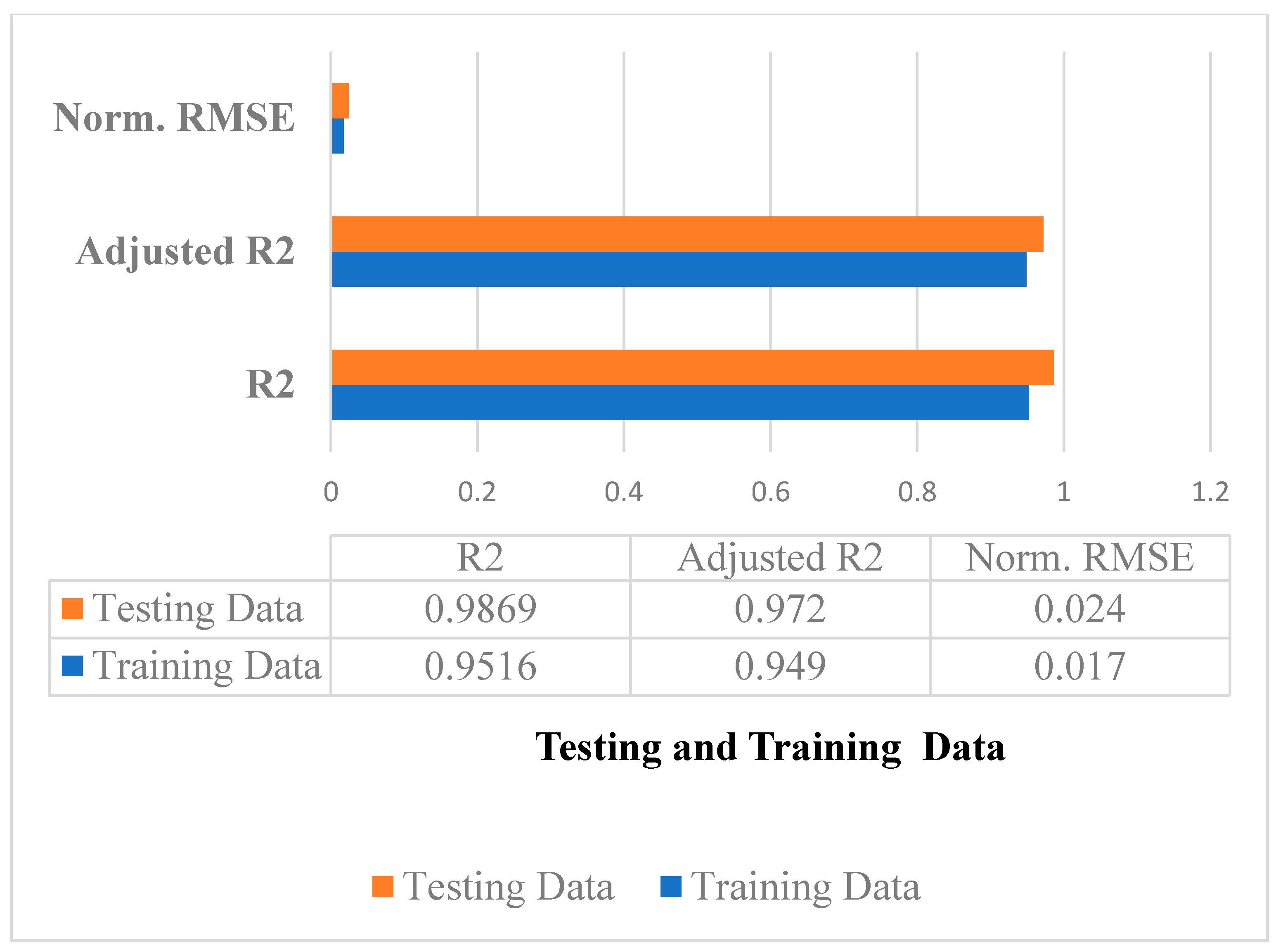
- Performance Accuracy and Error Measures
- d.
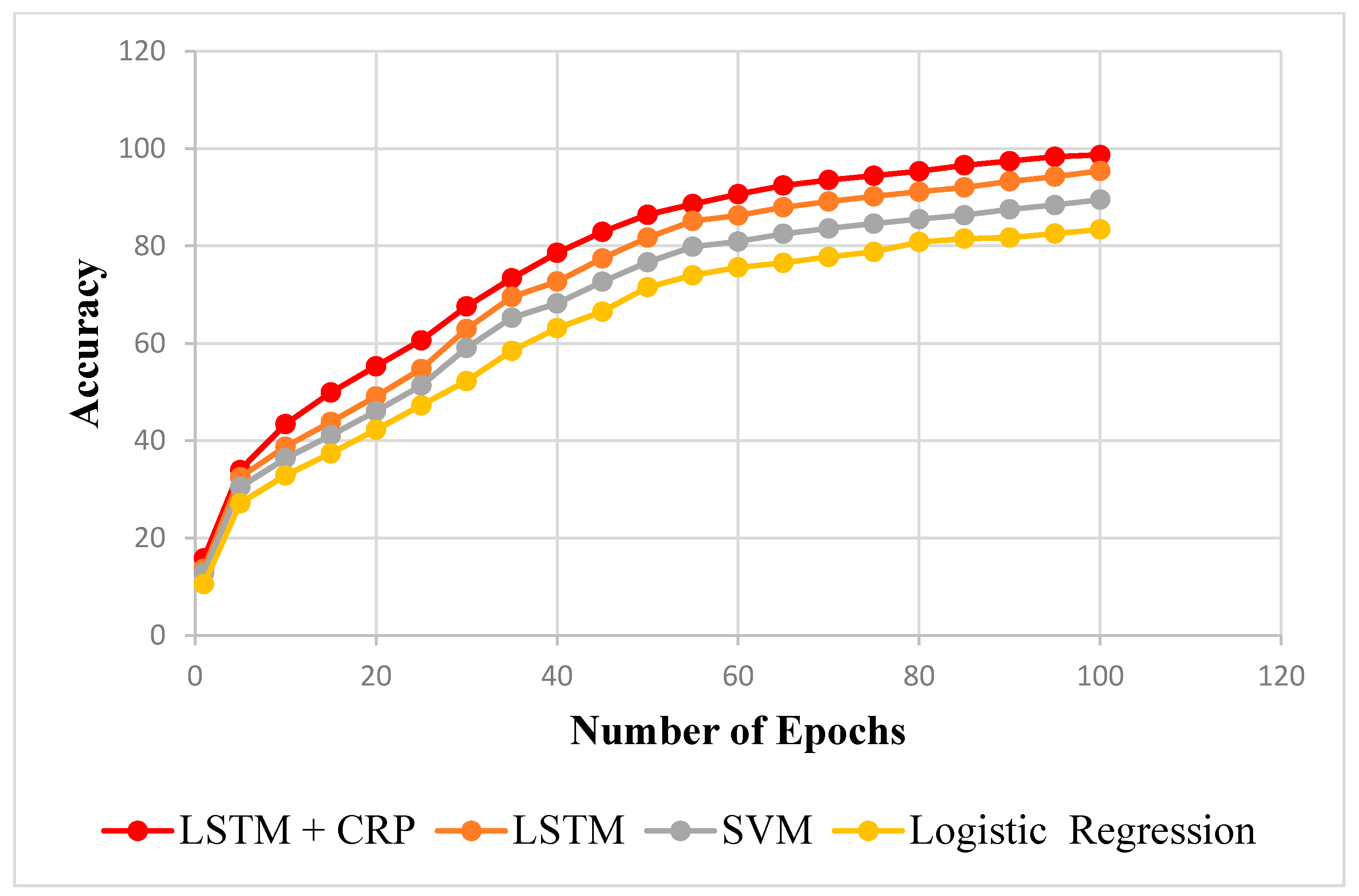
- Failure Prediction
5.3. Evaluation and Inference
- (a)
- Prediction of Minimum Delay
- (b)
- Processing Time
- (c)
- Accuracy and Error Measures
- (d)
- Failure Prediction
- (e)
- Significance Test Using Paired t-Test
6. Conclusions and Future Work
Author Contributions
Funding
Informed Consent Statement
Data Availability Statement
Acknowledgments
Conflicts of Interest
References
- Gubbi, J.; Buyya, R.; Marusic, S.; Palaniswami, M. Internet of Things (IoT): A vision, architectural elements, and future directions. Future Gener. Comput. Syst. 2013, 29, 1645–1660. [Google Scholar] [CrossRef] [Green Version]
- Botta, A.; De Donato, W.; Persico, V.; Pescapé, A. Integration of cloud computing and internet of things: A survey. Future Gener. Comput. Syst. 2016, 56, 684–700. [Google Scholar] [CrossRef]
- Bittencourt, F.L.; Rana, O.; Petri, I. Cloud computing at the edges. In International Conference on Cloud Computing and Services Science; Springer: Cham, Switzerland, 2015; pp. 3–12. [Google Scholar]
- Bonomi, F.; Milito, R.; Zhu, J.; Addepalli, S. Fog computing and its role in the internet of things. In Proceedings of the First Edition of the MCC Workshop on Mobile Cloud Computing, Helsinki, Finland, 17 August 2012; pp. 13–16. [Google Scholar]
- Vaquero, M.L.; Rodero-Merino, L.; Caceres, J.; Lindner, M. A break in the clouds: Towards a cloud definition. ACM Sigcomm Comput. Commun. Rev. 2008, 39, 50–55. [Google Scholar] [CrossRef] [Green Version]
- Sabireen, H.; Neelanarayanan, V. A review on fog computing: Architecture, fog with IoT, algorithms and research challenges. ICT Express 2021, 7, 162–176. [Google Scholar]
- Barroso, L.A.; Clidaras, J.; Hölzle, U. The datacenter as a computer: An introduction to the design of warehouse-scale machines. Synth. Lect. Comput. Archit. 2013, 8, 1–154. [Google Scholar]
- Oppenheimer, D.; Ganapathi, A.; Patterson, D.A. Why do Internet services fail, and what can be done about it? In 4th Usenix Symposium on Internet Technologies and Systems (USITS 03); USENIX Association: Berkeley, CA, USA, 2003. [Google Scholar]
- Hochreiter, S.; Bengio, Y.; Frasconi, P.; Schmidhuber, J. Gradient Flow in Recurrent Nets: The Difficulty of Learning Long-Term Dependencies; IEEE Press: Piscataway, NJ, USA, 2001. [Google Scholar]
- Graves, A.; Schmidhuber, J. Offline handwriting recognition with multidimensional recurrent neural networks. In Proceedings of the Advances in Neural Information Processing Systems 21, Vancouver, BC, Canada, 8–11 December 2008. [Google Scholar]
- Razgon, M.; Mousavi, A. Relaxed rule-based learning for automated predictive maintenance: Proof of concept. Algorithms 2020, 13, 219. [Google Scholar] [CrossRef]
- Mukwevho, M.A.; Celik, T. Toward a smart cloud: A review of fault-tolerance methods in cloud systems. IEEE Trans. Serv. Comput. 2018, 14, 589–605. [Google Scholar] [CrossRef]
- Tsigkanos, C.; Nastic, S.; Dustdar, S. Towards resilient internet of things: Vision, challenges, and research roadmap. In Proceedings of the 2019 IEEE 39th International Conference on Distributed Computing Systems (ICDCS), Dallas, TX, USA, 7–10 July 2019; pp. 1754–1764. [Google Scholar]
- Hasan, M.; Goraya, M.S. Fault tolerance in cloud computing environment: A systematic survey. Comput. Ind. 2018, 99, 156–172. [Google Scholar] [CrossRef]
- Sharif, A.; Nickray, M.; Shahidinejad, A. Energy-efficient fault-tolerant scheduling in a fog-based smart monitoring application. Int. J. Ad Hoc Ubiquitous Comput. 2021, 36, 32–49. [Google Scholar] [CrossRef]
- Ghobaei-Arani, M.; Souri, A.; Rahmanian, A.A. Resource management approaches in fog computing: A comprehensive review. J. Grid Comput. 2019, 18, 1–42. [Google Scholar] [CrossRef]
- Fu, S.; Xu, C.Z. Exploring event correlation for failure prediction in coalitions of clusters. In Proceedings of the 2007 ACM/IEEE Conference on Supercomputing, Reno, NV, USA, 10–16 November 2007; Volume 41, p. 112. [Google Scholar]
- Alarifi, A.; Abdelsamie, F.; Amoon, M. A fault-tolerant aware scheduling method for fog-cloud environments. PLoS ONE 2019, 14, e0223902. [Google Scholar] [CrossRef] [Green Version]
- Tajiki, M.M.; Shojafar, M.; Akbari, B.; Salsano, S.; Conti, M. Software defined service function chaining with failure consideration for fog computing. Concurr. Comput. Pract. Exp. 2019, 31, e4953. [Google Scholar] [CrossRef]
- Battula, S.K.; Garg, S.; Montgomery, J.; Kang, B.H. An efficient resource monitoring service for fog computing environments. IEEE Trans. Serv. Comput. 2019, 13, 709–722. [Google Scholar] [CrossRef]
- Zhang, J. Overview on Fault Tolerance Strategies of Composite Service in Service Computing. Wirel. Commun. Mob. Comput. 2018, 2018, 9787503. [Google Scholar] [CrossRef] [Green Version]
- Abdulhamid, S.M.; Latiff, M.S.A.; Madni, S.H.H.; Abdullahi, M. Fault tolerance aware scheduling technique for cloud computing environment using dynamic clustering algorithm. Neural Comput. Appl. 2018, 29, 279–293. [Google Scholar] [CrossRef]
- Amoon, M. A job checkpointing system for computational grids. Open Comput. Sci. 2013, 3, 17–26. [Google Scholar] [CrossRef] [Green Version]
- Liu, Y.; Fieldsend, J.; Min, G. A Framework of Fog Computing: Architecture, Challenges and Optimization. IEEE Access 2017, 5, 25445–25454. [Google Scholar] [CrossRef]
- Goiri, I.; Julià, F.; Guitart, J.; Torres, J. Checkpoint-based fault-tolerant infrastructure for virtualized service providers. In Proceedings of the 12th IEEE/IFIP Network Operations and Management Symposium (NOMS’10), Osaka, Japan, 19–23 April 2010; pp. 455–462. [Google Scholar]
- Cao, J.; Simonin, M.; Cooperman, G.; Morin, C. Checkpointing as a service in heterogeneous cloud environments. In Proceedings of the 15th IEEE/ACM International Symposium on Cluster, Cloud and Grid Computing, Shenzhen, China, 4–7 May 2015; pp. 61–70. [Google Scholar]
- Abdulhamid, S.; Abd Latiff, M.A. Checkpointed League Championship Algorithm-Based Cloud Scheduling Scheme with Secure Fault Tolerance Responsiveness. Appl. Soft Comput. 2017, 61, 670–680. [Google Scholar] [CrossRef]
- Louatia, T.; Abbesa, H.; Ce´rinb, C.; Jemnia, M. LXCloud-CR: Towards LinuX Containers Distributed Hash Table based Checkpoint-Restart. J. Parallel Distrib. Comput. 2018, 111, 187–205. [Google Scholar] [CrossRef]
- Ozeer, U.; Etchevers, X.; Letondeur, L.; Ottogalli, F.-G.; Salaün, G.; Vincent, J.-M. Resilience of stateful IOT applications in a dynamic fog environment. In Proceedings of the 15th EAI International Conference on Mobile and Ubiquitous Systems: Computing, Networking and Services, New York, NY, USA, 5–7 November 2018; pp. 1–10. [Google Scholar]
- Souza, V.B.; Masip-Bruin, X.; Marín-Tordera, E.; Ramírez, W.; Sánchez-López, S. Proactive vs. reactive failure recovery assessment in combined fog-to-cloud (F2C) systems. In Proceedings of the IEEE 22nd International Workshop on Computer Aided Modeling and Design of Communication Links and Networks (CAMAD), Lund, Sweden, 19–21 June 2017; pp. 1–5. [Google Scholar]
- Takami, G.; Tokuoka, M.; Goto, H.; Nozaka, Y. Machine learning applied to sensor data analysis. Yokogawa Tech. Rep. Engl. 2016, 59, 27–30. [Google Scholar]
- Sahoo, S.K.; Rodriguez, P.; Savinovic, D. 2015 IEEE International Electric Machines & Drives Conference (IEMDC); IEEE: Piscataway, NJ, USA, 2015; pp. 1398–1404. [Google Scholar]
- Fürnkranz, J.; Gamberger, D.; Lavrač, N. Foundations of Rule Learning; Springer Science & Business Media: Berlin/Heidelberg, Germany, 2012. [Google Scholar]
- Park, D.; Kim, S.; An, Y.; Jung, J.-Y. LiReD: A light-weight real-time fault detection system for edge computing using LSTM recurrent neural networks. Sensors 2018, 18, 2110. [Google Scholar] [CrossRef] [PubMed] [Green Version]
- Hochreiter, S.; Schmidhuber, J. Long short-term memory. Neural Comput. 1997, 9, 1735–1780. [Google Scholar] [CrossRef] [PubMed]
- Gers, A.F.; Schmidhuber, J.; Cummins, F. Learning to forget: Continual prediction with LSTM. Neural Comput. 2000, 12, 2451–2471. [Google Scholar] [CrossRef]
- Cortez, B.; Carrera, B.; Kim, Y.-J.; Jung, J.-Y. An architecture for emergency event prediction using LSTM recurrent neural networks. Expert Syst. Appl. 2018, 97, 315–324. [Google Scholar] [CrossRef]
- Ross, S. A First Course in Probability, 8th ed.; Pearson: London, UK, 2009. [Google Scholar]
- Schroeder, B.; Gibson, G.A. A large-scale study of failures in high-performance computing systems. IEEE Trans. Dependable Secur. Comput. 2009, 7, 337–350. [Google Scholar] [CrossRef]
- Heath, T.; Martin, R.P.; Nguyen, T.D. Improving cluster availability using workstation validation. In Proceedings of the 2002 ACM Sigmetrics International Conference on Measurement and Modeling of Computer Systems, Marina Del Rey, CA, USA, 15–19 June 2002; pp. 217–227. [Google Scholar]
- Sahoo, K.R.; Squillante, M.S.; Sivasubramaniam, A.; Zhang, Y. Failure data analysis of a large-scale heterogeneous server environment. In Proceedings of the International Conference on Dependable Systems and Networks, Florence, Italy, 28 June–1 July 2004; pp. 772–781. [Google Scholar]
- iFogSim Toolkit. Available online: https://github.com/Cloudslab/iFogSim (accessed on 29 August 2021).
- Awaisi, K.S.; Abbas, A.; Zareei, M.; Khattak, H.A.; Khan, M.U.S.; Ali, M.; Din, I.U.; Shah, S. Towards a fog enabled efficient car parking architecture. IEEE Access 2019, 7, 159100–159111. [Google Scholar] [CrossRef]
- Aazam, M.; St-Hilaire, M.; Lung, C.-H.; Lambadaris, I. Cloud-based smart waste management for smart cities. In Proceedings of the 2016 IEEE 21st International Workshop on Computer Aided Modelling and Design of Communication Links and Networks (CAMAD), Toronto, ON, Canada, 23–25 October 2016; pp. 188–193. [Google Scholar] [CrossRef]
- Afrin, M.; Jin, J.; Rahman, A.; Tian, Y.-C.; Kulkarni, A. Multi-objective resource allocation for Edge Cloud based robotic workflow in smart factory. Future Gener. Comput. Syst. 2019, 97, 119–130. [Google Scholar] [CrossRef]
- Awaisi, K.S.; Abbas, A.; Khan, S.U.; Mahmud, R.; Buyya, R. Simulating Fog Computing Applications using iFogSim Toolkit. In Mobile Edge Computing; Springer: Cham, Germany, 2021; pp. 565–590. [Google Scholar] [CrossRef]
- Naha, R.K.; Garg, S.; Chan, A.; Battula, S.K. Deadline-based dynamic resource allocation and provisioning algorithms in fog-cloud environment. Future Gener. Comput. Syst. 2020, 104, 131–141. [Google Scholar] [CrossRef]
- Naha, R.K.; Garg, S. Multi-criteria--based Dynamic User Behaviour--aware Resource Allocation in Fog Computing. ACM Trans. Int. Things 2021, 2, 1–31. [Google Scholar] [CrossRef]
- Yu, Y.; Si, X.; Hu, C.; Zhang, J. A review of recurrent neural networks: LSTM cells and network architectures. Neural Comput. 2019, 31, 1235–1270. [Google Scholar] [CrossRef]
- Kwon, J.-H.; Kim, E.-J. Failure prediction model using iterative feature selection for industrial internet of things. Symmetry 2020, 12, 454. [Google Scholar] [CrossRef] [Green Version]
- Manoharan, H.; Teekaraman, Y.; Kirpichnikova, I.; Kuppusamy, R.; Nikolovski, S.; Baghaee, H.R. Smart grid monitoring by wireless sensors using binary logistic regression. Energies 2020, 13, 3974. [Google Scholar] [CrossRef]


| Fog Node Parameters | Description |
|---|---|
| FN_VM | Fog node virtual machine |
| FN_VMR | Fog node new virtual machine request for compute and storage resources |
| FNA_C+S | Fog node availability of computation and storage resources (CPU + RAM) |
| FN_UD | Fog node of uplink and downlink |
| FN_level | The level of the fog node |
| FN_pow | Fog node Power contains the busy power and idle power in watts |
| H_PR | The request which performs critical data processing and needs good response time |
| Y | IoT Applications |
| Y_C+S | Compute and storage resource requirements of each IoT application |
| R_CoFN | Fog node cost of a VM, when it is reallocated or rescheduled to another node |
| Schedule_Queue | VM requests are rescheduled back when their resources are available |
| FN_fault | The fog node does not cater to the needs of the IoT application and is not tolerable to faults and must be rescheduled from the queue |
| IoT_pow | IoT application requirement of power consumption |
| System Device | Parameter | Value |
|---|---|---|
| Fog Nodes | Total fog nodes | 10–25 |
| Each Fog Node | Total VMs | 2 |
| RAM (unit) | 128–4000 (Mbps) | |
| CPU processing power (unit) | 1000–2800 (MIPS) | |
| Power capacity (units) | 1 (watt) | |
| Data storage capacity (unit) | 1 (GB) | |
| The capacity of bandwidth (unit) | 100–10,000 (Mbps) | |
| Total CPUs | 1 | |
| OS | Linux | |
| VMM–Hypervisor | Xen | |
| Data Center | Data center | 1 |
| Hosts | 1 |
| Parameter | IoT Applications Executed | Components of IoT Applications Length (MI) | File Size (MB) | Output Memory Size (MB) |
|---|---|---|---|---|
| Value | 3–5 | 250–950 | 100–1550 | 15–55 |
| MIPS | RAM | Upload Bw | Download Bw | Level | Busy Power | Idle Power | Available CPU | Available Ram |
|---|---|---|---|---|---|---|---|---|
| 44,800 | 16,000 | 100 | 10,000 | 0 | 1648 | 1332 | 2963.54 | 2073.37 |
| 2800 | 4000 | 10,000 | 10,000 | 1 | 106.339 | 63.67 | 2096.65 | 3074.78 |
| 2800 | 4000 | 10,000 | 10,000 | 1 | 97.339 | 84.54 | 623.48 | 1558.45 |
| 2800 | 4000 | 100 | 50 | 1 | 87.339 | 72.4333 | 2696.33 | 2135.91 |
| 1000 | 512 | 50 | 10 | 0 | 107.339 | 62.54 | 1581.53 | 3771.31 |
| 2000 | 750 | 8500 | 8500 | 1 | 97.349 | 82.5333 | 1723.21 | 1327.88 |
| 2000 | 1000 | 9000 | 8500 | 1 | 103.539 | 83.4333 | 965.55 | 2998.68 |
| 1500 | 3500 | 9500 | 9500 | 1 | 101.9 | 63.4333 | 2639.47 | 3801.73 |
| 2300 | 3300 | 7500 | 6000 | 1 | 91.339 | 83.4333 | 2695.63 | 1556.61 |
| 1750 | 3800 | 7600 | 7550 | 0 | 107.549 | 83.4333 | 797.44 | 3258.75 |
| 2100 | 2000 | 2000 | 1900 | 1 | 78.339 | 83.4333 | 677.98 | 3370.15 |
| Epochs | LSTM + CRP | LSTM | SVM | Logistic Regression |
|---|---|---|---|---|
| 10 | 41.8608 | 37.0656 | 35.6928 | 32.5523 |
| 35 | 70.7184 | 66.4632 | 64.0016 | 57.8932 |
| 50 | 83.322 | 78.0948 | 75.2024 | 70.8313 |
| 55 | 85.4496 | 81.3672 | 78.3536 | 73.2553 |
| 70 | 90.2016 | 85.1796 | 82.0248 | 76.9923 |
| 75 | 91.0548 | 86.1948 | 83.0024 | 78.0225 |
| 90 | 93.9384 | 89.1648 | 85.8624 | 80.9212 |
| 95 | 94.824 | 90.072 | 86.736 | 81.7292 |
| 100 | 95.1696 | 91.206 | 87.828 | 82.5978 |
| Epochs | LSTM + CRP | LSTM | SVM | Logistic Regression |
|---|---|---|---|---|
| 10 | 43.4112 | 38.7816 | 36.3792 | 32.8746 |
| 35 | 73.3376 | 69.5402 | 65.2324 | 58.4664 |
| 50 | 86.408 | 81.7103 | 76.6486 | 71.5326 |
| 55 | 88.6144 | 85.1342 | 79.8604 | 73.9806 |
| 70 | 93.5424 | 89.1231 | 83.6022 | 77.7546 |
| 75 | 94.4272 | 90.1853 | 84.5986 | 78.795 |
| 90 | 97.4176 | 93.2928 | 87.5136 | 81.7224 |
| 95 | 98.336 | 94.242 | 88.404 | 82.5384 |
| 100 | 98.6944 | 95.4285 | 89.517 | 83.4156 |
| Fog Nodes | Time (Mins) | MTTR | MTBF | Ava Avgr | fpa | n_fp |
|---|---|---|---|---|---|---|
| 20 | 50 | 0.11 | 888.43 | 99.98 | 98.2 | 2 |
| 100 | 0.19 | 976.12 | 99.98 | 97.7 | 5 | |
| 150 | 0.21 | 1001.89 | 99.89 | 99.2 | 8 | |
| 200 | 0.09 | 1078.45 | 99.99 | 98.5 | 11 | |
| 40 | 50 | 0.31 | 1011.21 | 99.96 | 98.3 | 4 |
| 100 | 0.28 | 1078.92 | 99.99 | 97.4 | 9 | |
| 150 | 0.21 | 1103.53 | 99.99 | 99.1 | 13 | |
| 200 | 0.19 | 1179.28 | 99.98 | 97.4 | 18 | |
| 60 | 50 | 0.42 | 1202.16 | 99.96 | 98.5 | 7 |
| 100 | 0.37 | 1276.29 | 99.97 | 99.7 | 16 | |
| 150 | 0.33 | 1329.03 | 99.97 | 97.3 | 22 | |
| 200 | 0.30 | 1399.45 | 99.97 | 97.7 | 31 | |
| 80 | 50 | 0.54 | 1448.91 | 99.96 | 98.4 | 12 |
| 100 | 0.41 | 1496.29 | 99.97 | 96.6 | 19 | |
| 150 | 0.38 | 1521.28 | 99.97 | 97.3 | 29 | |
| 200 | 0.33 | 1535.74 | 99.97 | 98.7 | 45 | |
| 100 | 50 | 0.78 | 1623.12 | 99.95 | 98.3 | 19 |
| 100 | 0.62 | 1622.88 | 99.96 | 98.8 | 26 | |
| 150 | 0.57 | 1705.28 | 99.96 | 99.4 | 49 | |
| 200 | 0.41 | 1794.48 | 99.97 | 98.1 | 62 |
| Accuracy of the Proposed Approach | Accuracy of the LSTM Approach | |
|---|---|---|
| Mean | 0.98 | 0.84 |
| Observations | 5 | 5 |
| Variance | 0.0001 | 0.0009 |
| Mean Difference Hypothesized | 0 | - |
| df | 2 | - |
| Pearson Correlation | −0.16423367 | - |
| t Stat | 4.6690876545 | - |
| One tail when P(T ≤ t) | 0.08679823 | - |
| Two tail when P(T ≤ t) | 0.17895624 | - |
| T critical two tail | 3.3198679 | - |
Disclaimer/Publisher’s Note: The statements, opinions and data contained in all publications are solely those of the individual author(s) and contributor(s) and not of MDPI and/or the editor(s). MDPI and/or the editor(s) disclaim responsibility for any injury to people or property resulting from any ideas, methods, instructions or products referred to in the content. |
© 2023 by the authors. Licensee MDPI, Basel, Switzerland. This article is an open access article distributed under the terms and conditions of the Creative Commons Attribution (CC BY) license (https://creativecommons.org/licenses/by/4.0/).
Share and Cite
H, S.; Venkataraman, N. Proactive Fault Prediction of Fog Devices Using LSTM-CRP Conceptual Framework for IoT Applications. Sensors 2023, 23, 2913. https://doi.org/10.3390/s23062913
H S, Venkataraman N. Proactive Fault Prediction of Fog Devices Using LSTM-CRP Conceptual Framework for IoT Applications. Sensors. 2023; 23(6):2913. https://doi.org/10.3390/s23062913
Chicago/Turabian StyleH, Sabireen, and Neelanarayanan Venkataraman. 2023. "Proactive Fault Prediction of Fog Devices Using LSTM-CRP Conceptual Framework for IoT Applications" Sensors 23, no. 6: 2913. https://doi.org/10.3390/s23062913