
Integrated Probe System for Measuring Soil Carbon Dioxide Concentrations
 , and
, and 
Abstract
:1. Introduction
2. Materials and Methods
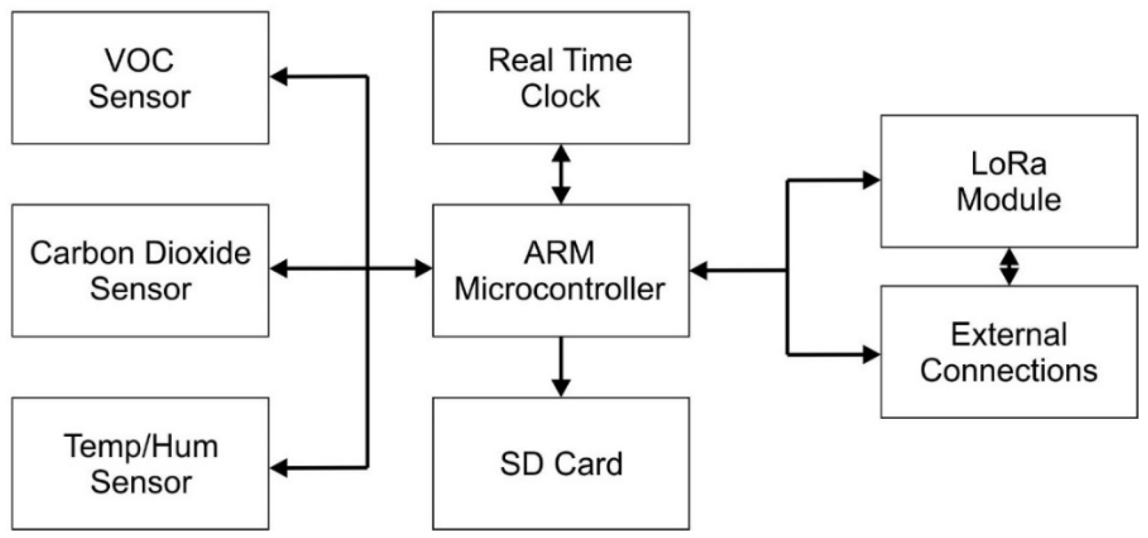
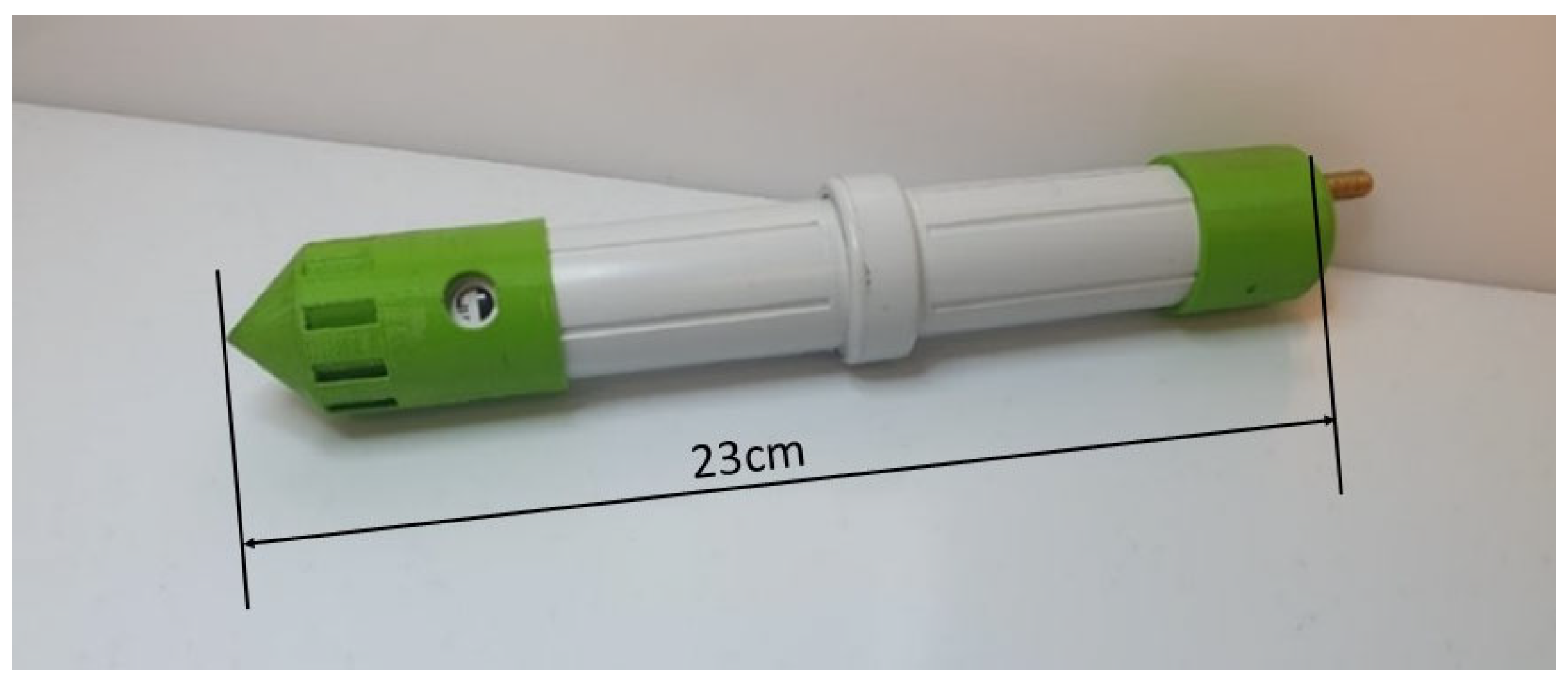
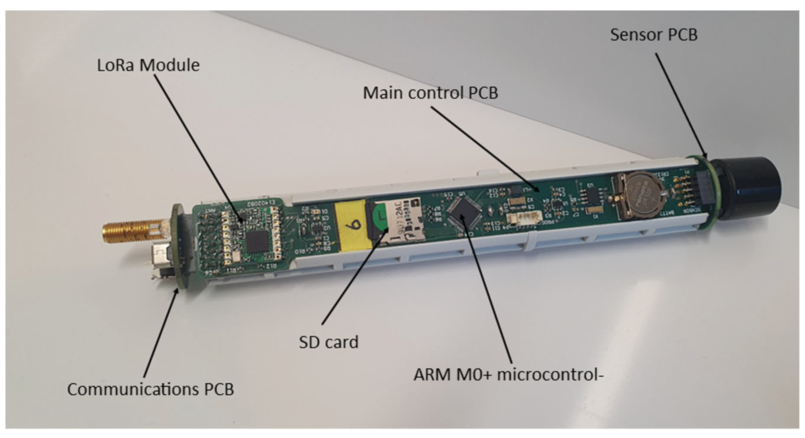
2.1. Sensor Probe
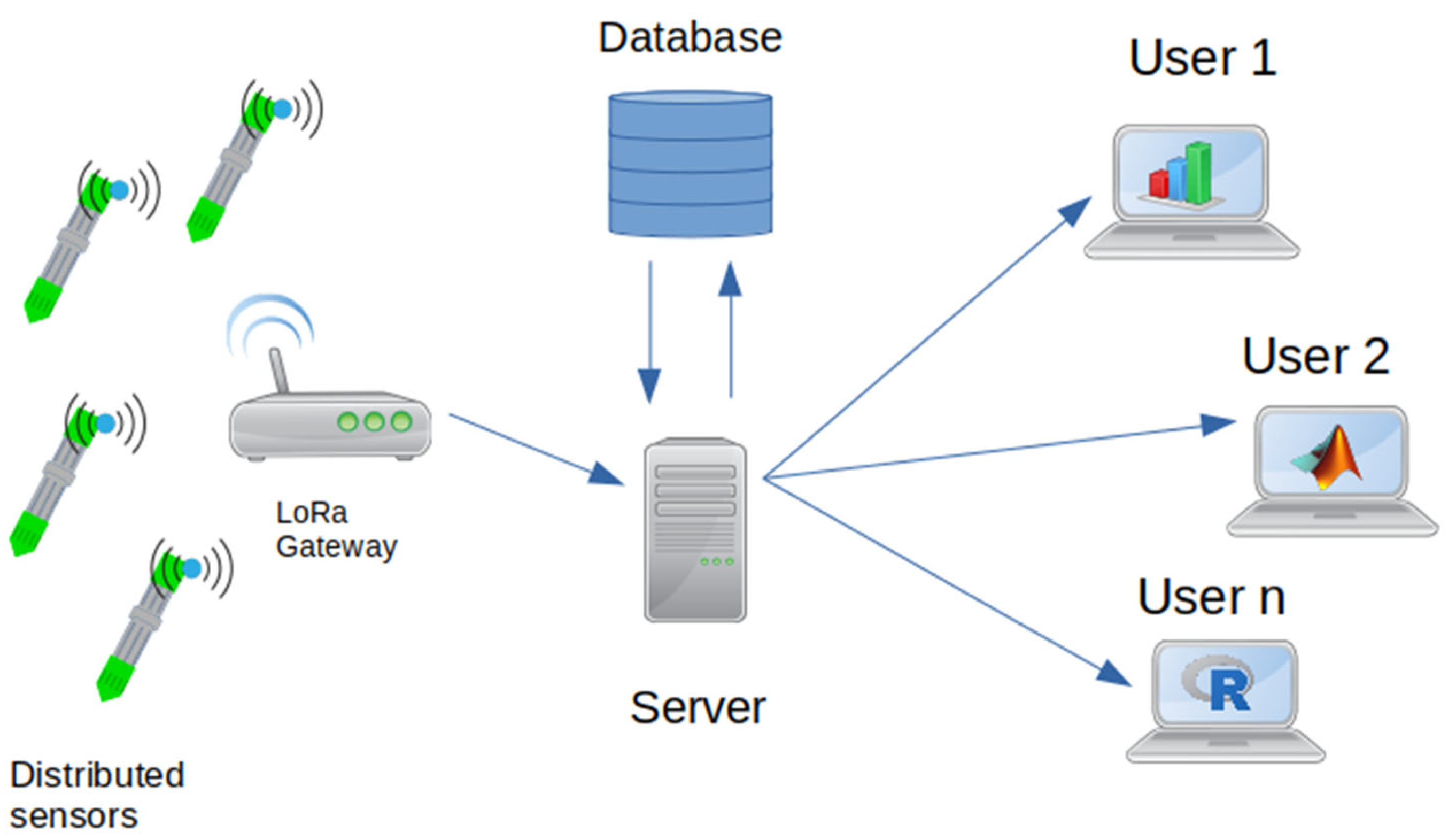
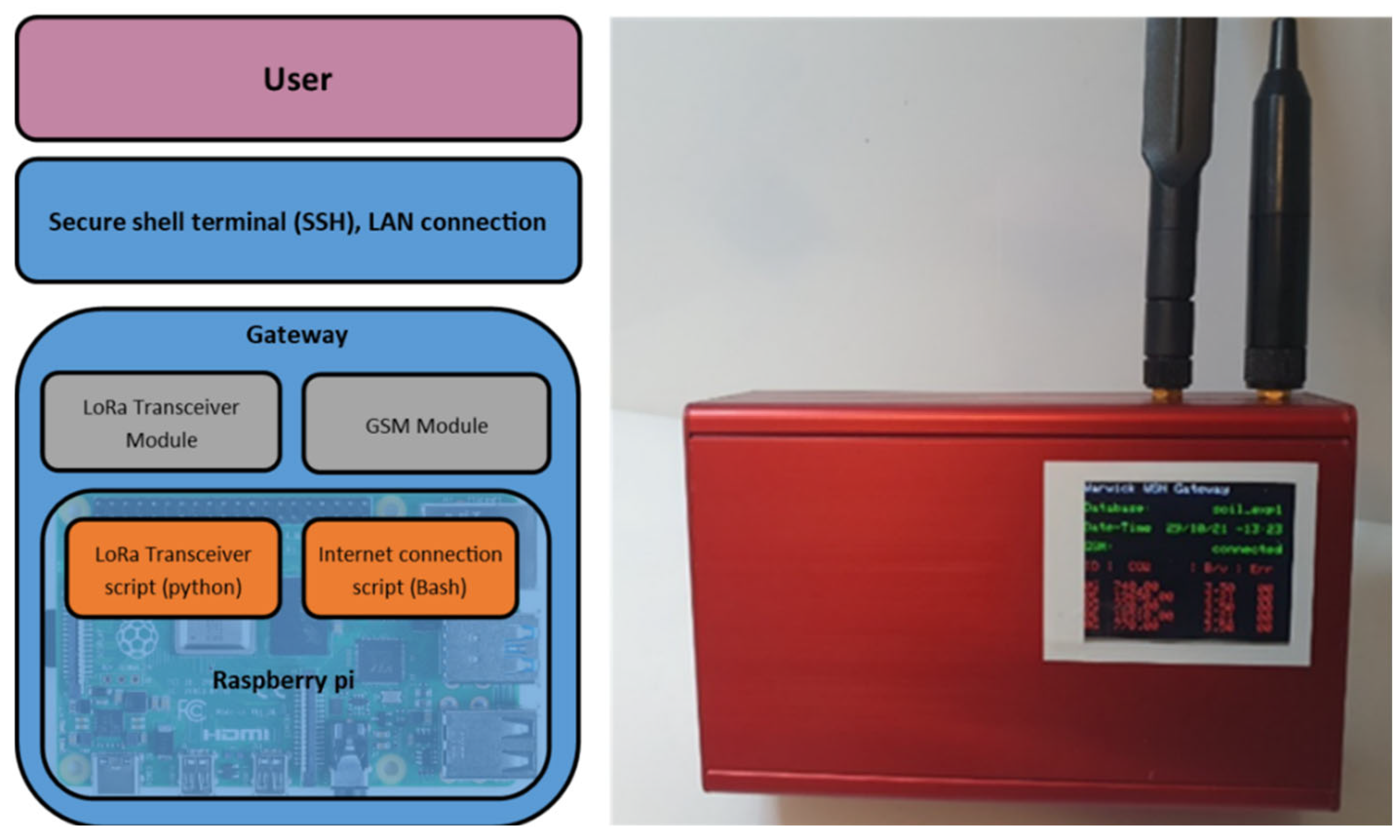
2.2. Gateway
2.3. Data storage and Dashboard
2.4. Experimental Method
2.4.1. Deployment 1
2.4.2. Deployment 2
2.4.3. Deployment 3
3. Results
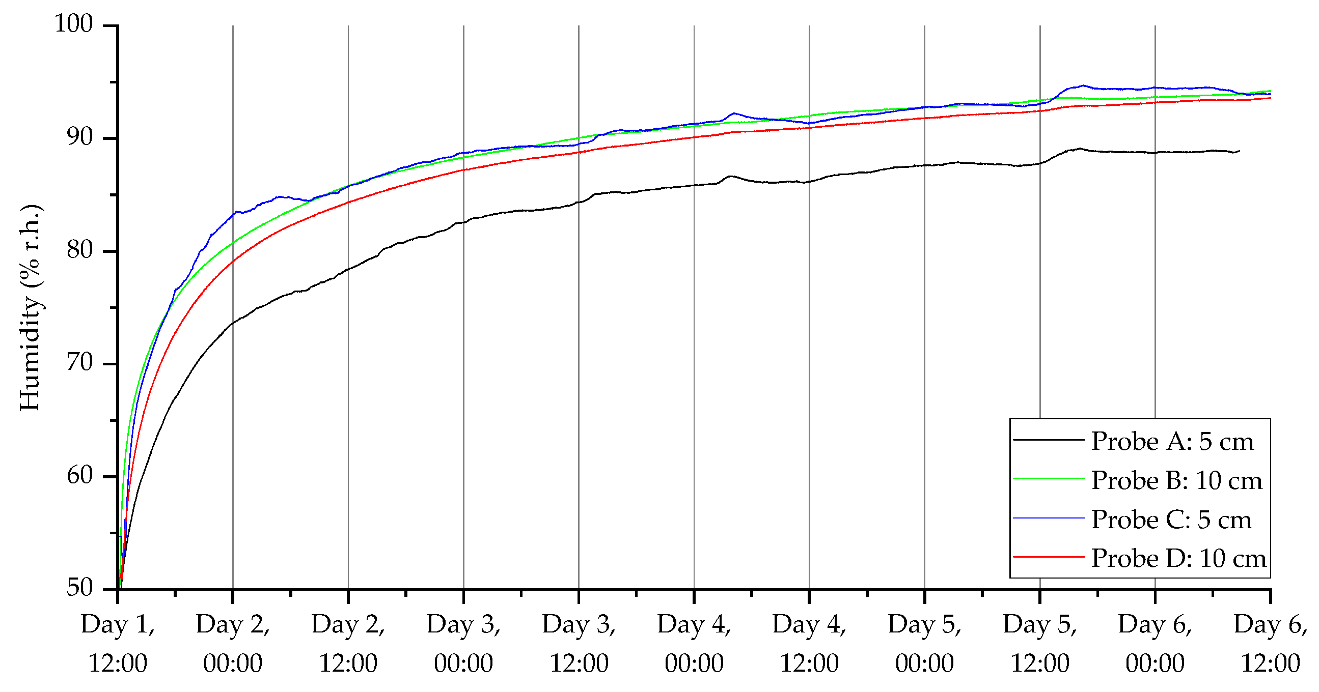
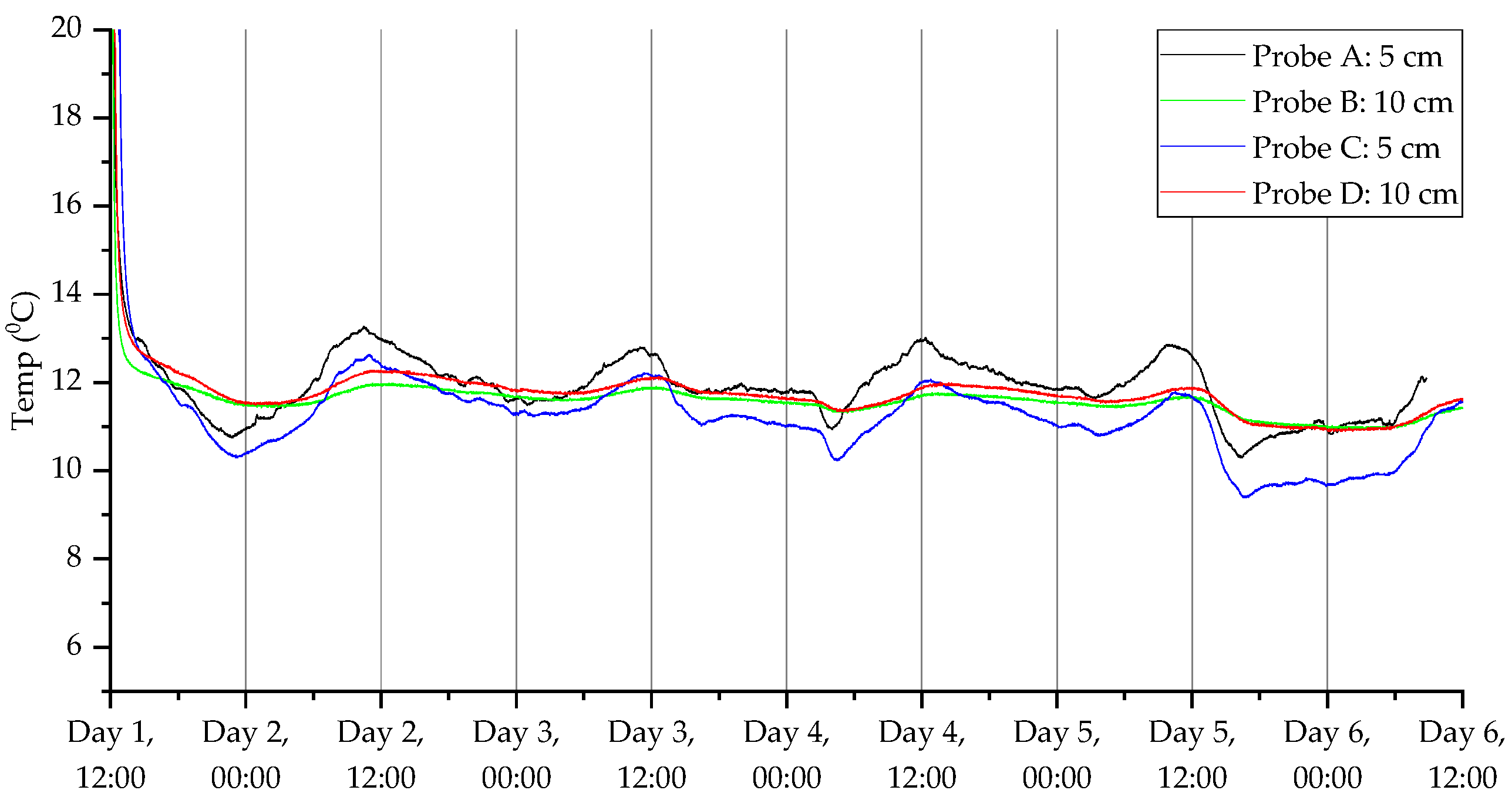
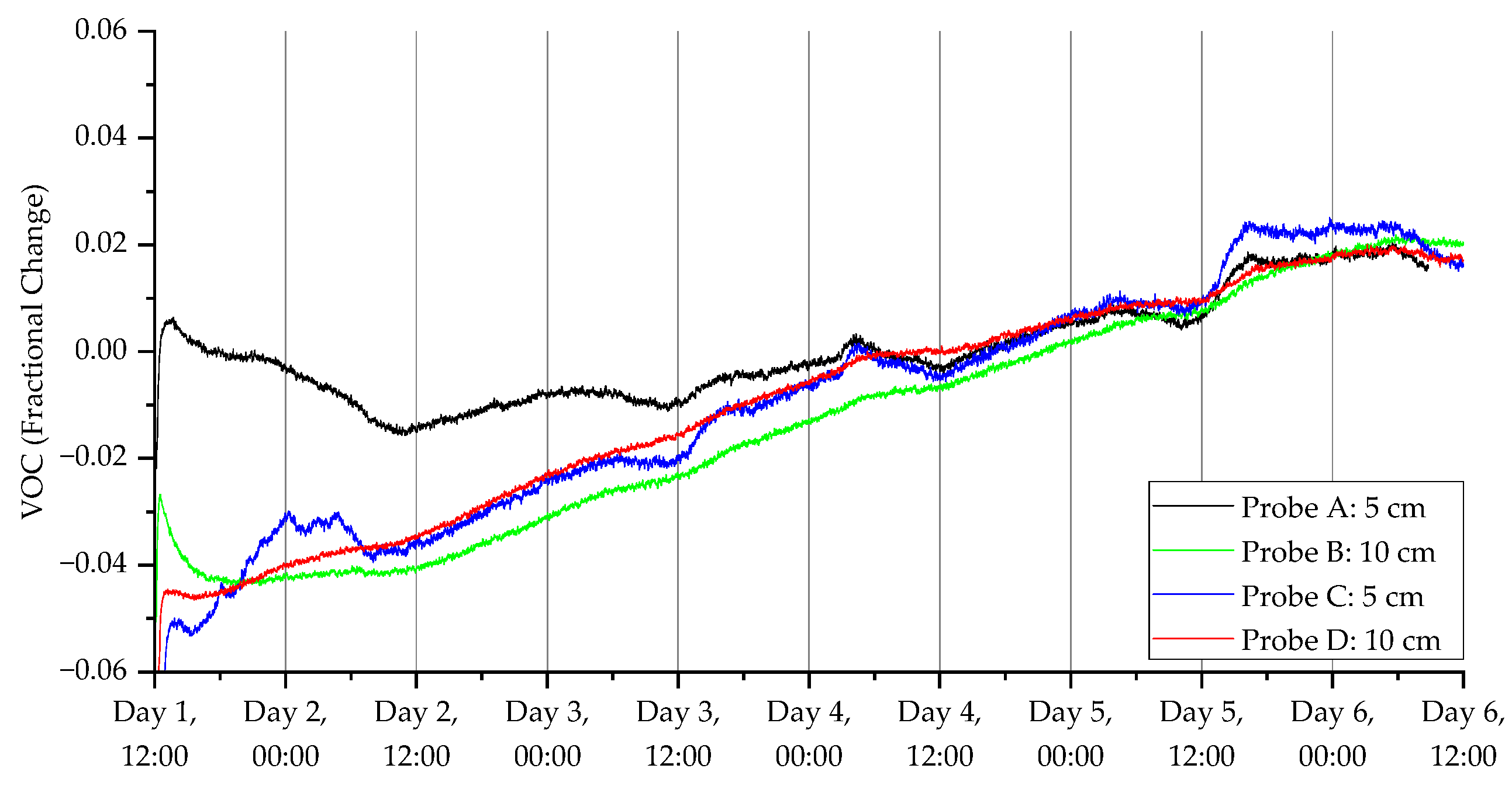
3.1. Deployment 1
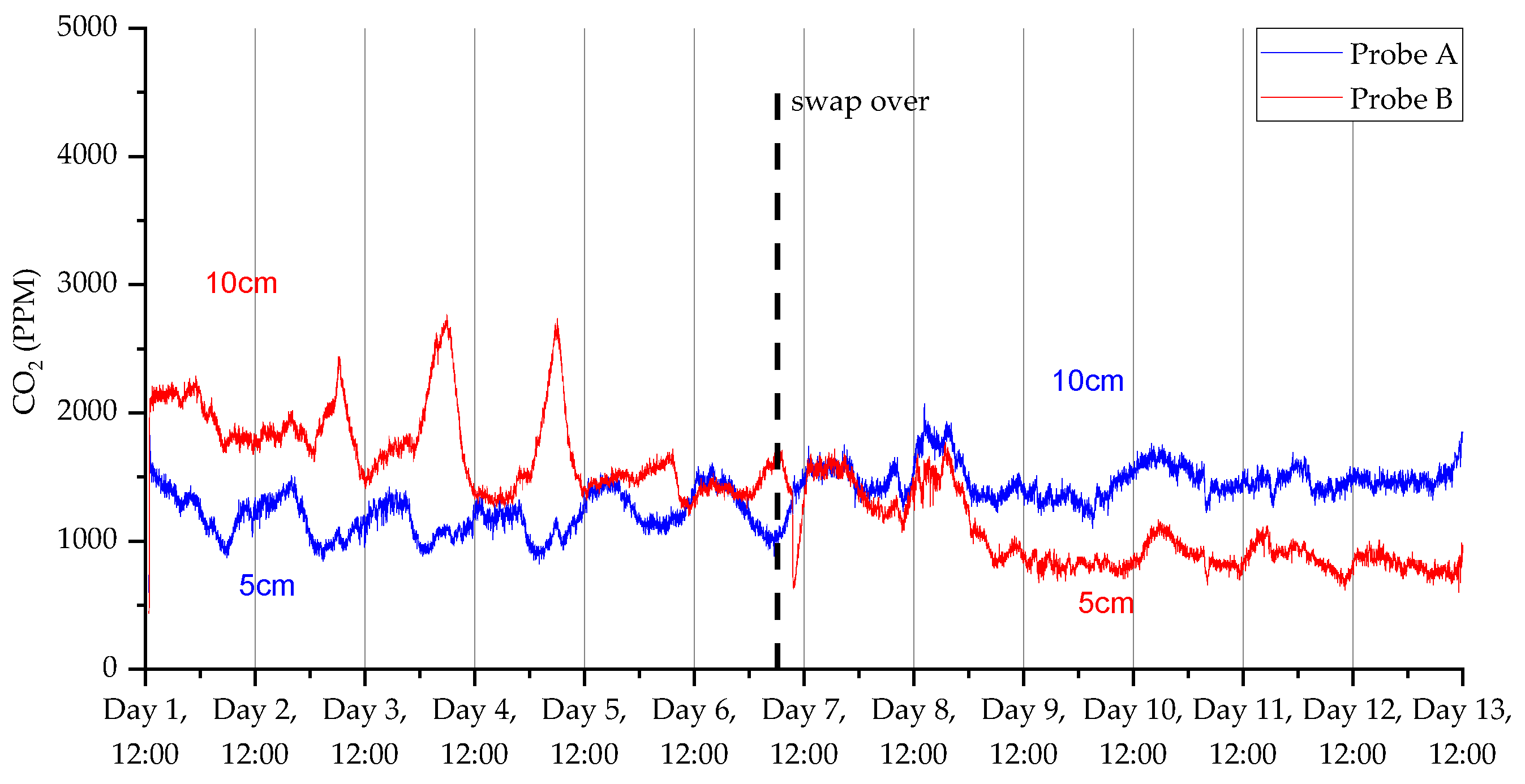
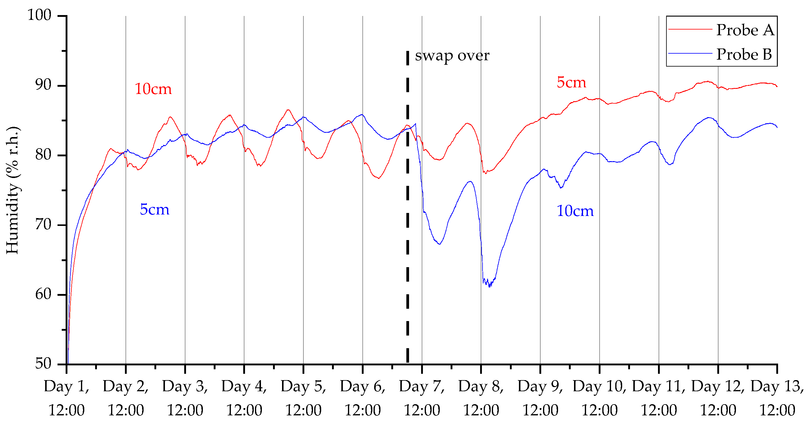
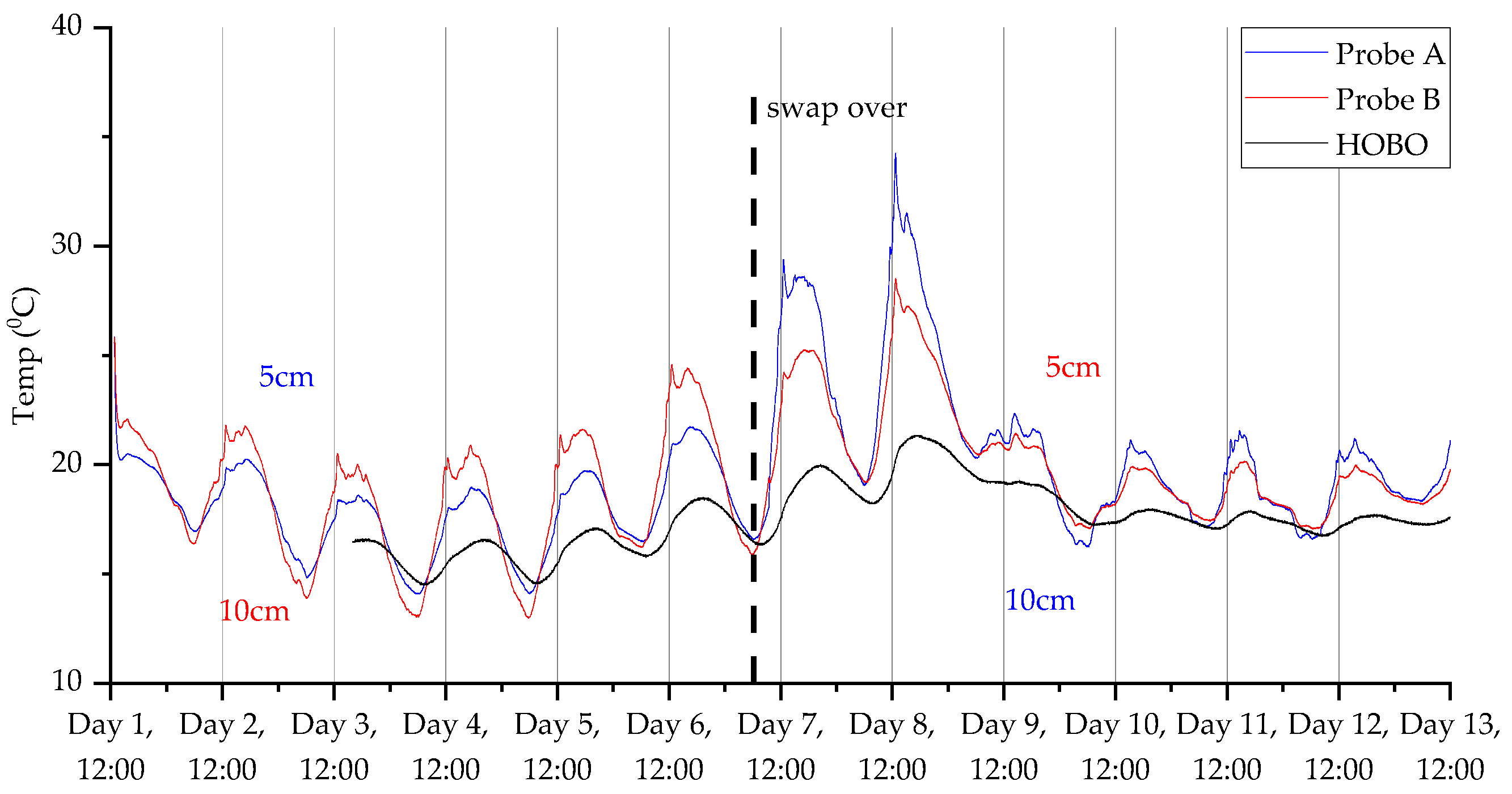
3.2. Deployment 2
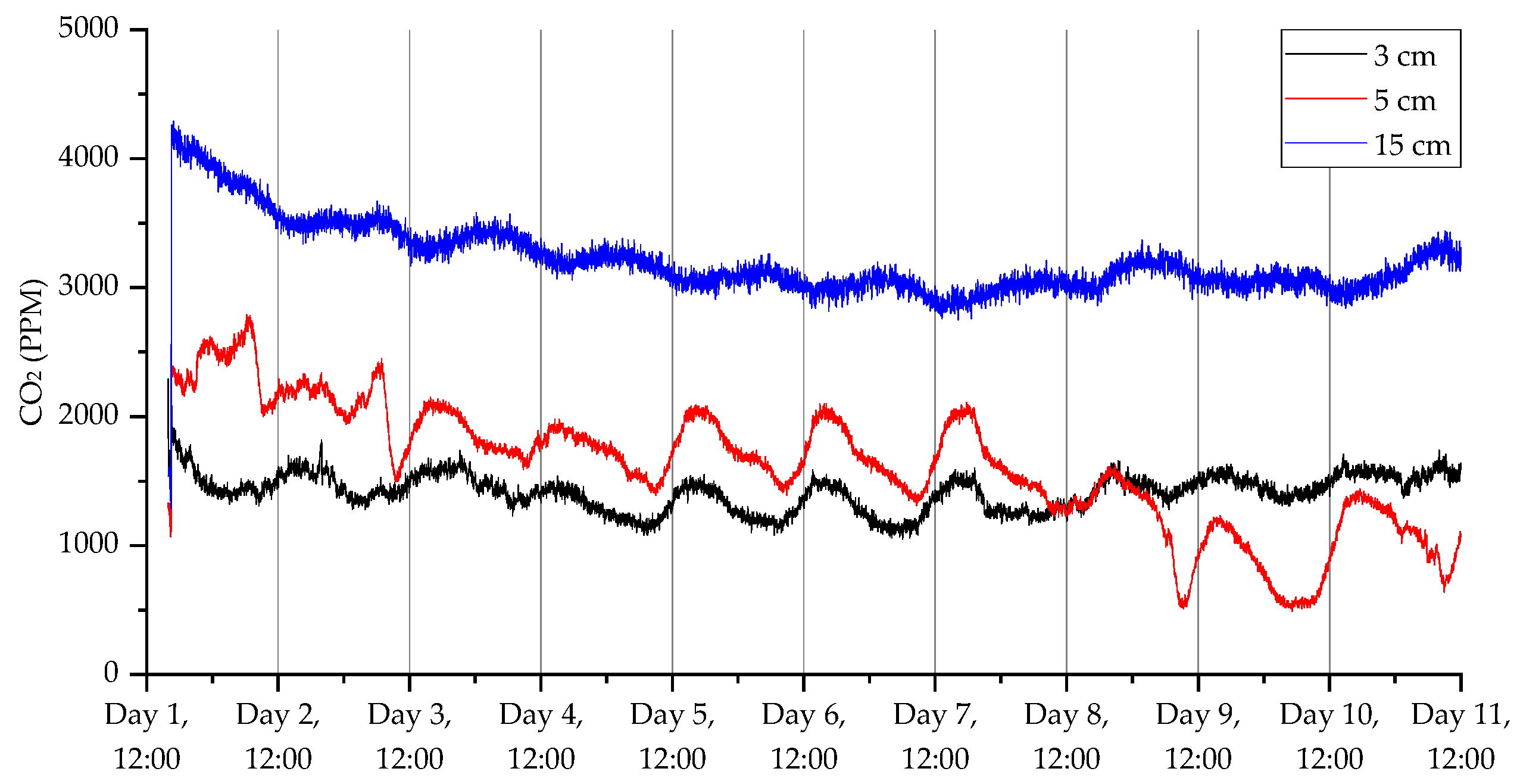
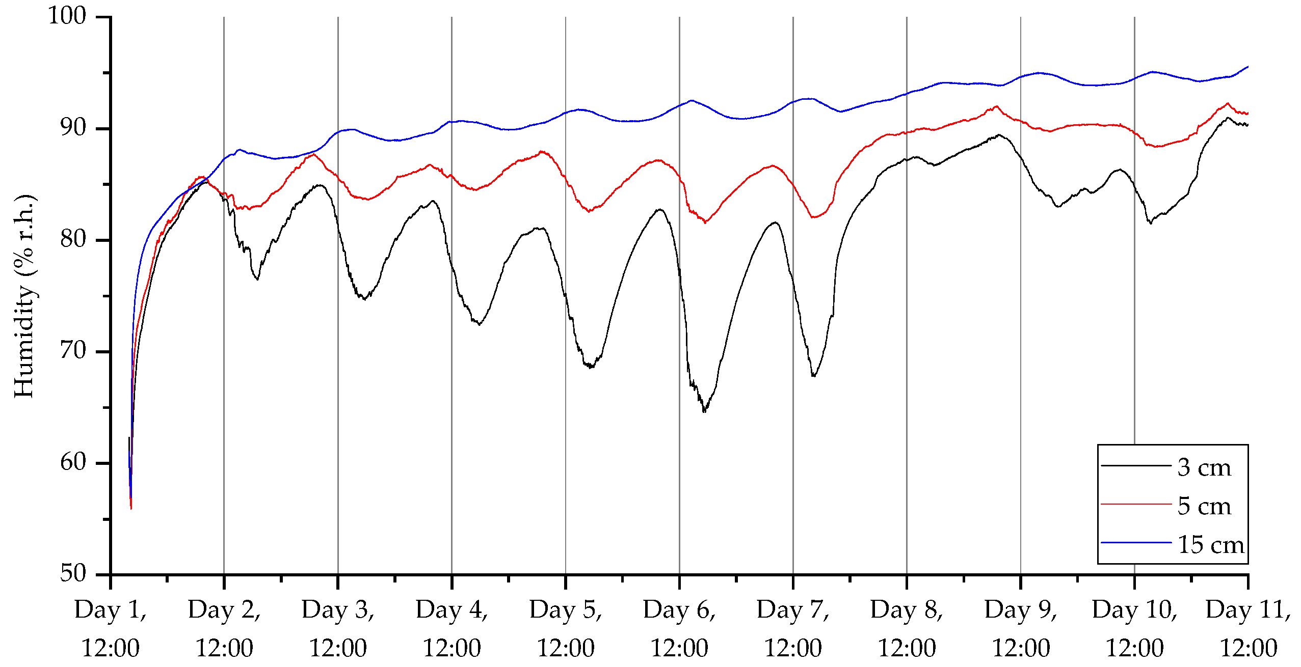
3.3. Deployment 3
4. Discussion
5. Conclusions
Author Contributions
Funding
Data Availability Statement
Conflicts of Interest
References
- Malhi, Y. The concept of the Anthropocene. Annu. Rev. Environ. Resour. 2017, 42, 77–104. [Google Scholar] [CrossRef] [Green Version]
- Shukla, P.R.; Skeg, J.; Buendia, E.C.; Masson-Delmotte, V.; Pörtner, H.O.; Roberts, D.C.; Zhai, P.; Slade, R.; Connors, S.; Van Diemen, S.; et al. Climate Change and Land: An IPCC Special Report on Climate Change, Desertification, Land Degradation, Sustainable Land Management, Food Security, and Greenhouse Gas Fluxes in Terrestrial Ecosystems; IPCC: Geneva, Switzerland, 2019. [Google Scholar]
- Kuzyakov, Y. Sources of CO2 efflux from soil and review of partitioning methods. Soil Biol. Biochem. 2006, 38, 425–448. [Google Scholar] [CrossRef]
- Pumpanen, J.; Kolari, P.; Ilvesniemi, H.; Minkkinen, K.; Vesala, T.; Niinistö, S.; Lohila, A.; Larmola, T.; Morero, M.; Pihlatie, M.; et al. Comparison of different chamber techniques for measuring soil CO2 efflux. Agric. For. Meteorol. 2004, 123, 159–176. [Google Scholar] [CrossRef]
- Anthony, T.L.; Silver, W.L. Hot moments drive extreme nitrous oxide and methane emissions from agricultural peatlands. Glob. Change Biol. 2021, 27, 5141–5153. [Google Scholar] [CrossRef]
- Gulati, K.; Boddu, R.S.K.; Kapila, D.; Bangare, S.L.; Chandnani, N.; Saravanan, G. A review paper on wireless sensor network techniques in Internet of Things (IoT). Mater. Today Proc. 2021, 51, 161–165. [Google Scholar] [CrossRef]
- Al-Qurabat, A.K.M.; Abdulzahra, S.A. An overview of periodic wireless sensor networks to the internet of things. IOP Conf. Ser. Mater. Sci. Eng. 2020, 928, 032055. [Google Scholar] [CrossRef]
- Antolín, D.; Medrano, N.; Calvo, B.; Pérez, F. A wearable wireless sensor network for indoor smart environment monitoring in safety applications. Sensors 2017, 17, 365. [Google Scholar] [CrossRef]
- Al-Qurabat, A.K.M.; Abou Jaoude, C.; Idrees, A.K. Two tier data reduction technique for reducing data transmission in IoT sensors. In Proceedings of the 15th International Wireless Communications & Mobile Computing Conference (IWCMC), Tangier, Morocco, 24–28 June 2019; pp. 168–173. [Google Scholar] [CrossRef]
- Mohammad, G.B.; Shitharth, S. Wireless sensor network and IoT based systems for healthcare application. Mater. Today Proc. 2020, 63, 20827–20837. [Google Scholar] [CrossRef]
- Vijayalakshmi, J.; Puthilibhai, G.; Siddarth, S.L. Implementation of Ammonia Gas Leakage Detection & Monitoring System using Internet of Things. In Proceedings of the Third International conference on I-SMAC (IoT in Social, Mobile, Analytics and Cloud)(I-SMAC), Palladam, India, 12–14 December 2019; pp. 778–781. [Google Scholar] [CrossRef]
- Jelicic, V.; Magno, M.; Brunelli, D.; Paci, G.; Benini, L. Context-adaptive multimodal wireless sensor network for energy-efficient gas monitoring. IEEE Sens. J. 2012, 13, 328–338. [Google Scholar] [CrossRef]
- Raghuveera, E.; Kanakaraja, P.; Kishore, K.H.; Sriya, C.T.; Lalith, B.S.K.T. An IoT Enabled Air Quality Monitoring System Using LoRa and LPWAN. In Proceedings of the 5th International Conference on Computing Methodologies and Communication (ICCMC), Erode, India, 8–10 April 2021; pp. 453–459. [Google Scholar] [CrossRef]
- Wu, F.; Rüdiger, C.; Redouté, J.M.; Yuce, M.R. WE-Safe: A wearable IoT sensor node for safety applications via LoRa. In Proceedings of the IEEE 4th World Forum on Internet of Things (WF-IoT), Singapore, 5–8 February 2018; pp. 144–148. [Google Scholar] [CrossRef]
- Moharana, B.K.; Anand, P.; Kumar, S.; Kodali, P. Development of an IoT-based real-time air quality monitoring device. In Proceedings of the International Conference on Communication and Signal Processing (ICCSP), Chennai, India, 28–30 July 2020; pp. 191–194. [Google Scholar] [CrossRef]
- Jia, Y. LoRa-based WSNs construction and low-power data collection strategy for wetland environmental monitoring. Wirel. Pers. Commun. 2020, 114, 1533–1555. [Google Scholar] [CrossRef]
- Rachmani, A.F.; Zulkifli, F.Y. Design of iot monitoring system based on lora technology for starfruit plantation. In Proceedings of the TENCON IEEE Region 10 Conference, Jeju, Republic of Korea, 28–31 October 2018; pp. 1241–1245. [Google Scholar] [CrossRef]
- Ramson, S.J.; León-Salas, W.D.; Brecheisen, Z.; Foster, E.J.; Johnston, C.T.; Schulze, D.G.; Filley, T.; Rahimi, R.; Soto, M.J.C.V.; Bolivar, J.A.L.; et al. A self-powered, real-time, LoRaWAN IoT-based soil health monitoring system. IEEE Internet Things J. 2021, 8, 9278–9293. [Google Scholar] [CrossRef]
- Toschke, Y.; Lusmoeller, J.; Otte, L.; Schmidt, J.; Meyer, S.; Tessmer, A.; Brockmann, C.; Ahuis, M.; Hüer, E.; Kirberger, C.; et al. Distributed LoRa based CO2 monitoring network–A standalone open source system for contagion prevention by controlled ventilation. HardwareX 2022, 11, e00261. [Google Scholar] [CrossRef]
- Wu, F.; Wu, T.; Yuce, M.R. An internet-of-things (IoT) network system for connected safety and health monitoring applications. Sensors 2018, 19, 21. [Google Scholar] [CrossRef] [Green Version]
- Muosa, A.H.; Hamed, A.M. Remote Monitoring and Smart Control System for Greenhouse Environmental and Automation Irrigations Based on WSNs and GSM Module. IOP Conf. Ser. Mater. Sci. Eng. 2020, 928, 032037. [Google Scholar] [CrossRef]
- García, L.; Parra, L.; Jimenez, J.M.; Parra, M.; Lloret, J.; Mauri, P.V.; Lorenz, P. Deployment strategies of soil monitoring WSN for precision agriculture irrigation scheduling in rural areas. Sensors 2021, 21, 1693. [Google Scholar] [CrossRef]
- Parmar, G.; Lakhani, S.; Chattopadhyay, M.K. An IoT based low cost air pollution monitoring system. In Proceedings of the International Conference on Recent Innovations in Signal processing and Embedded Systems (RISE), Bhopal, India, 27–29 October 2017; pp. 524–528. [Google Scholar] [CrossRef]
- Fastellini, G.; Schillaci, C. Precision farming and IoT case studies across the world. In Agricultural Internet of Things and Decision Support for Precision Smart Farming; Elsevier: Amsterdam, The Netherlands, 2020; pp. 331–415. [Google Scholar] [CrossRef]
- Fahmi, N.; Prayitno, E.; Fitriani, S. Web of Thing Application for Monitoring Precision Agriculture Using Wireless Sensor Network. J. Infotel 2019, 11, 22–28. [Google Scholar] [CrossRef]
- Gaikwad, S.V.; Vibhute, A.D.; Kale, K.V.; Mehrotra, S.C. An innovative IoT based system for precision farming. Comput. Electron. Agric. 2021, 187, 106291. [Google Scholar] [CrossRef]
- Xu, J.; Zhang, J.; Zheng, X.; Wei, X.; Han, J. Wireless sensors in farmland environmental monitoring. In Proceedings of the International Conference on Cyber-Enabled Distributed Computing and Knowledge Discovery, Xi’an, China, 17–19 September 2015; pp. 372–379. [Google Scholar] [CrossRef]
- Díaz, S.E.; Pérez, J.C.; Mateos, A.C.; Marinescu, M.C.; Guerra, B.B. A novel methodology for the monitoring of the agricultural production process based on wireless sensor networks. Comput. Electron. Agric. 2011, 76, 252–265. [Google Scholar] [CrossRef]
- Geetha, D.M.; Chitra, P.; Umamaheswari, M.; Naveen, P.; Nagaraj, V. Smart fertilizer management system based on IoT chlorophyll meter. Mater. Today Proc. 2020. [Google Scholar] [CrossRef]
- Ramadhan, A.S.; Abdurohman, M.; Putrada, A.G. WSN based agricultural bird pest control with buzzer and a mesh network. In Proceedings of the 8th International Conference on Information and Communication Technology (ICoICT), Yogyakarta, Indonesia, 24–26 June 2020; pp. 1–5. [Google Scholar] [CrossRef]
- Azfar, S.; Nadeem, A.; Basit, A. Pest detection and control techniques using wireless sensor network: A review. J. Entomol. Zool. Stud. 2015, 3, 92–99. [Google Scholar]
- AdelineSneha, J.; Chakravarthi, R.; Glenn, J.A. A review on energy efficient image feature transmission in WSN for micro region pest control. In Proceedings of the International Conference on Electrical, Electronics, and Optimization Techniques (ICEEOT), Chennai, India, 3–5 March 2016; pp. 4859–4862. [Google Scholar] [CrossRef]
- Wani, H.; Ashtankar, N. An appropriate model predicting pest/diseases of crops using machine learning algorithms. In Proceedings of the 4th International Conference on Advanced Computing and Communication Systems (ICACCS), Coimbatore, India, 6–7 January 2017; pp. 1–4. [Google Scholar] [CrossRef]
- Liqiang, Z.; Shouyi, Y.; Leibo, L.; Zhen, Z.; Shaojun, W. A crop monitoring system based on wireless sensor network. Procedia Environ. Sci. 2011, 11, 558–565. [Google Scholar] [CrossRef] [Green Version]
- Maimaitijiang, M.; Sagan, V.; Sidike, P.; Daloye, A.M.; Erkbol, H.; Fritschi, F.B. Crop monitoring using satellite/UAV data fusion and machine learning. Remote Sens. 2020, 12, 1357. [Google Scholar] [CrossRef]
- Schirrmann, M.; Giebel, A.; Gleiniger, F.; Pflanz, M.; Lentschke, J.; Dammer, K.H. Monitoring agronomic parameters of winter wheat crops with low-cost UAV imagery. Remote Sens. 2016, 8, 706. [Google Scholar] [CrossRef] [Green Version]
- Chebrolu, N.; Läbe, T.; Stachniss, C. Robust long-term registration of UAV images of crop fields for precision agriculture. IEEE Robot. Autom. Lett. 2018, 3, 3097–3104. [Google Scholar] [CrossRef]
- Mahmud, M.A.; Buyamin, S.; Mokji, M.M.; Abidin, M.Z. Internet of things based smart environmental monitoring for mushroom cultivation. Indones. J. Electr. Eng. Comput. Sci. 2020, 10, 847–852. [Google Scholar] [CrossRef]
- Faiazuddin, S.; Lakshmaiah, M.V.; Alam, K.T.; Ravikiran, M. IoT based Indoor Air Quality Monitoring system using Raspberry Pi4. In Proceedings of the 4th International Conference on Electronics, Communication and Aerospace Technology (ICECA), Coimbatore, India, 5–7 November 2020; pp. 714–719. [Google Scholar] [CrossRef]
- Lee, M.; Kim, H.K.; Yoe, H. Smart Cattle Shed Monitoring System in LoRa Network. In Software Engineering in IoT, Big Data, Cloud and Mobile Computing; Springer: Berlin/Heidelberg, Germany, 2020; pp. 141–152. [Google Scholar] [CrossRef]
- Available online: https://www.vaisala.com/en/products/instruments-sensors-and-other-measurement-devices/instruments-industrial-measurements/gmp343 (accessed on 23 November 2022).
- Available online: https://eosense.com/products/ (accessed on 23 November 2022).
- Maier, M.; Schack-Kirchner, H. Using the gradient method to determine soil gas flux: A review. Agric. For. Meteorol. 2014, 192, 78–95. [Google Scholar] [CrossRef]
- Nakadai, T.; Yokozawa, M.; Ikeda, H.; Koizumi, H. Diurnal changes of carbon dioxide flux from bare soil in agricultural field in Japan. Appl. Soil Ecol. 2002, 19, 161–171. [Google Scholar] [CrossRef]
- Choudoir, M.; Rossabi, S.; Gebert, M.; Helmig, D.; Fierer, N. A phylogenetic and functional perspective on volatile organic compound production by actinobacteria. MSystems 2019, 4, e00295-18. [Google Scholar] [CrossRef] [Green Version]
- Zaman, M.; Kleineidam, K.; Bakken, L.; Berendt, J.; Bracken, C.; Butterbach-Bahl, K.; Cai, Z.; Chang, S.X.; Clough, T.; Dawar, K.; et al. Methodology for measuring greenhouse gas emissions from agricultural soils using non-isotopic techniques. In Measuring Emission of Agricultural Greenhouse Gases and Developing Mitigation Options Using Nuclear and Related Techniques; Springer Nature: Berlin/Heidelberg, Germany, 2021; pp. 11–108. [Google Scholar]
- NEON (National Ecological Observatory Network). Soil CO2 Concentration (DP1.00095.001), RELEASE-2022. Available online: https://data.neonscience.org (accessed on 21 November 2022).
- Makita, N.; Kosugi, Y.; Sakabe, A.; Kanazawa, A.; Ohkubo, S.; Tani, M. Seasonal and diurnal patterns of soil respiration in an evergreen coniferous forest: Evidence from six years of observation with automatic chambers. PLoS ONE 2018, 13, e0192622. [Google Scholar] [CrossRef] [Green Version]
- Newman, A.; Picot, E.; Davies, S.; Hilton, S.; Carré, I.A.; Bending, G.D. Circadian rhythms in the plant host influence rhythmicity of rhizosphere microbiota. BMC Biol. 2022, 20, 235. [Google Scholar] [CrossRef]


| Part/Supplier | Specification | Purpose |
|---|---|---|
| ExplorIR-M, GSS, UK | 0–5% CO2 ±(70 ppm, +5%) | Carbon dioxide NDIR Sensor |
| SHT31, Sensirion, Switzerland | ±2 @0–100% RH ±0.2 @0–90 °C | Temperature and humidity sensor |
| SGP40 Sensirion, Switzerland | 0 to 1000 ppm of ethanol equivalents | Total VOC sensor |
| ATSAMD21G, Microchip | ARM M0+ | Microcontroller |
| PCF8523T/NXP | Year, month, day, weekday, hours, minutes, and seconds | Real-time clock |
| RFM96W, Sparkfun | LoRa 433 MHz | Communication unit |
| Device | Program | Function | Access |
|---|---|---|---|
| Probe | Data logger | Log data from sensor Send using Lora comms | Local, USB—serial port |
| Gateway | LoRa transceiver | To receive data from probes To separate data into headings and data types Send data using http request to API | One-way, updated by downloading remote repository Secure shell terminal, LAN connection |
| Gateway | Internet connection | Monitor internet connection Renew IP lease upon expiry | One-way, updated by downloading remote repository Secure shell terminal, LAN connection |
| Server | API | Check legitimacy of incoming data Send conformation back to gateway Insert data to correct table Manage data requests from website | Secure shell login, wan |
| Server | MySQL Database | Store data | Terminal login DBeaver user interface MySQL workbench |
| Server | Website | View data from database | Secure shell login ftp server Fasthosts dashboard |
| eosGP CO2 [48] | Vaisala GMP343 [47] | Warwick CO2 Probe | |
|---|---|---|---|
| Dimensions [Len, Dia] | 216 mm × 51 mm | 194 mm × 55 mm | 230 mm × 32 mm |
| Weight | 400 g | 360 g | 172 g |
| Operating power | 400 mW | <3500 mW | ~20 mW |
| Sensor technology | NDIR | NDIR | NDIR |
| Sensor Range | 0–30,000 ppm | 0–20,000 ppm | 0–50,000 ppm |
| Accuracy | ±3.5% of reading | ±5 ppm ±2% of reading | ±70 ppm |
| Communication Interface | RS485/analogue 0–5 v | RS485/RS232 | LoRa/UART USB |
| Battery life | Mains | Mains | 14 Days |
| Response time T90 | <90 s | 82 s | 22 s |
Disclaimer/Publisher’s Note: The statements, opinions and data contained in all publications are solely those of the individual author(s) and contributor(s) and not of MDPI and/or the editor(s). MDPI and/or the editor(s) disclaim responsibility for any injury to people or property resulting from any ideas, methods, instructions or products referred to in the content. |
© 2023 by the authors. Licensee MDPI, Basel, Switzerland. This article is an open access article distributed under the terms and conditions of the Creative Commons Attribution (CC BY) license (https://creativecommons.org/licenses/by/4.0/).
Share and Cite
Hassan, S.; Mushinski, R.M.; Amede, T.; Bending, G.D.; Covington, J.A. Integrated Probe System for Measuring Soil Carbon Dioxide Concentrations. Sensors 2023, 23, 2580. https://doi.org/10.3390/s23052580
Hassan S, Mushinski RM, Amede T, Bending GD, Covington JA. Integrated Probe System for Measuring Soil Carbon Dioxide Concentrations. Sensors. 2023; 23(5):2580. https://doi.org/10.3390/s23052580
Chicago/Turabian StyleHassan, Sammy, Ryan M. Mushinski, Tilahun Amede, Gary D. Bending, and James A. Covington. 2023. "Integrated Probe System for Measuring Soil Carbon Dioxide Concentrations" Sensors 23, no. 5: 2580. https://doi.org/10.3390/s23052580