Author Contributions
Conceptualization, K.V. and M.C.; methodology, K.V., C.H. and M.C.; software, K.V.; measurements, C.H., validation, K.V. and M.C.; supervision, M.C., writing—original draft preparation, K.V. and M.C.; writing—review and editing, K.V., C.H. and M.C.; All authors have read and agreed to the published version of the manuscript.
Figure 1.
(a) Antenna design transversal view; (b) Cross section of the coaxial cable used for the design; (c) Geometry of the simulations. Metal parts are represented in yellow, while the insulation materials are represented in blue.
Figure 1.
(a) Antenna design transversal view; (b) Cross section of the coaxial cable used for the design; (c) Geometry of the simulations. Metal parts are represented in yellow, while the insulation materials are represented in blue.
Figure 2.
(a) Realization of the applicator; (b) measurement setup with the antenna immersed into the liquid-filled tank.
Figure 2.
(a) Realization of the applicator; (b) measurement setup with the antenna immersed into the liquid-filled tank.
Figure 3.
(a) Equivalent circuit of the S&S de-embedding model; (b) Equivalent circuit of the M&E de-embedding model.
Figure 3.
(a) Equivalent circuit of the S&S de-embedding model; (b) Equivalent circuit of the M&E de-embedding model.
Figure 4.
Simulated and measured reflection coefficients in dB for (a) open circuit, (b) deionized water, (c) 0.1 mol NaCl solution, (d) 2 mol NaCl solution.
Figure 4.
Simulated and measured reflection coefficients in dB for (a) open circuit, (b) deionized water, (c) 0.1 mol NaCl solution, (d) 2 mol NaCl solution.
Figure 5.
S&S de-embedding of DW with OC, 0.1 mol and 2 mol NaCl; comparison between simulations and measurements: (a) ε′; (b) ε″.
Figure 5.
S&S de-embedding of DW with OC, 0.1 mol and 2 mol NaCl; comparison between simulations and measurements: (a) ε′; (b) ε″.
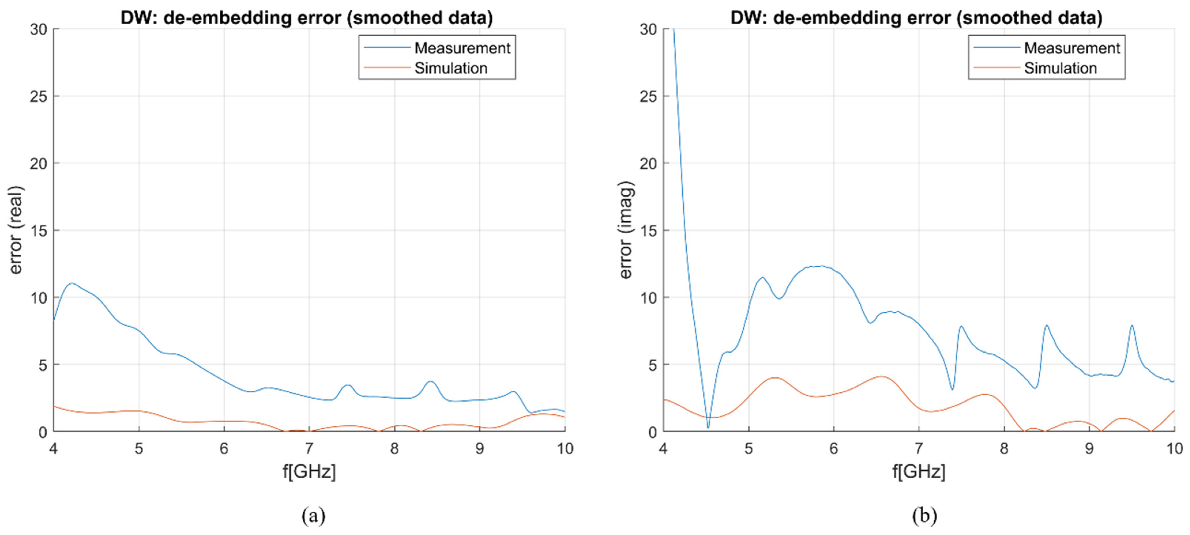
Figure 6.
Sensitivity (de-embedding error) comparison between simulation and measurement results: (a) ε′ (“real”); (b) ε″ (“imag”).
Figure 6.
Sensitivity (de-embedding error) comparison between simulation and measurement results: (a) ε′ (“real”); (b) ε″ (“imag”).
Figure 7.
S&S de-embedding with the 1st calibration option: OC, 0.1 mol and 2 mol NaCl (smoothing applied): (a) Calculated vs. reference ε′; (b) calculated vs. reference ε″; (c) sensitivity (de-embedding error) for ε′ (“real”) and ε″ (“imag”).
Figure 7.
S&S de-embedding with the 1st calibration option: OC, 0.1 mol and 2 mol NaCl (smoothing applied): (a) Calculated vs. reference ε′; (b) calculated vs. reference ε″; (c) sensitivity (de-embedding error) for ε′ (“real”) and ε″ (“imag”).
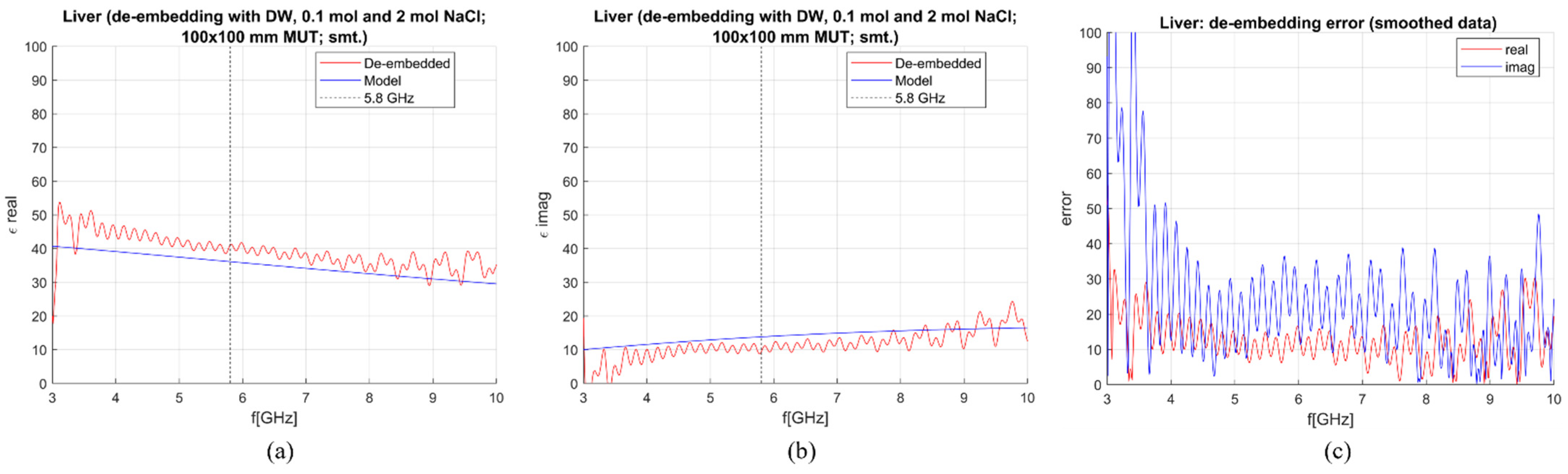
Figure 8.
S&S de-embedding with the 2nd calibration option: DW, 0.1 mol and 2 mol NaCl (smoothing applied): (a) Calculated vs. reference ε′; (b) calculated vs. reference ε″; (c) sensitivity (de-embedding error) for ε′ (“real”) and ε″ (“imag”).
Figure 8.
S&S de-embedding with the 2nd calibration option: DW, 0.1 mol and 2 mol NaCl (smoothing applied): (a) Calculated vs. reference ε′; (b) calculated vs. reference ε″; (c) sensitivity (de-embedding error) for ε′ (“real”) and ε″ (“imag”).
Figure 9.
S&S de-embedding with the 3rd calibration option: DW, 0.1 mol and 2 mol NaCl (smoothing applied): (a) Calculated vs. reference ε′; (b) calculated vs. reference ε″; (c) sensitivity (de-embedding error) for ε′ (“real”) and ε″ (“imag”).
Figure 9.
S&S de-embedding with the 3rd calibration option: DW, 0.1 mol and 2 mol NaCl (smoothing applied): (a) Calculated vs. reference ε′; (b) calculated vs. reference ε″; (c) sensitivity (de-embedding error) for ε′ (“real”) and ε″ (“imag”).
Figure 10.
S&S de-embedding with the 4th calibration option: DW, 1 mol NaCl and EG70 (smoothing applied): (a) Calculated vs. reference ε′; (b) calculated vs. reference ε″; (c) sensitivity (de-embedding error) for ε′ (“real”) and ε″ (“imag”).
Figure 10.
S&S de-embedding with the 4th calibration option: DW, 1 mol NaCl and EG70 (smoothing applied): (a) Calculated vs. reference ε′; (b) calculated vs. reference ε″; (c) sensitivity (de-embedding error) for ε′ (“real”) and ε″ (“imag”).
Figure 11.
Dielectric properties of different NaCl solutions, EG70, and liver: (a) ε′ and (b) σ.
Figure 11.
Dielectric properties of different NaCl solutions, EG70, and liver: (a) ε′ and (b) σ.
Figure 12.
M&E de-embedding with 1st calibration option; DW, OC, 0.1 mol and 2 mol NaCl (smoothing applied): (a) Calculated vs. reference ε′; (b) Calculated vs. reference ε″; (c) Sensitivity (de-embedding error) for ε′ (“real”) and ε″ (“imag”).
Figure 12.
M&E de-embedding with 1st calibration option; DW, OC, 0.1 mol and 2 mol NaCl (smoothing applied): (a) Calculated vs. reference ε′; (b) Calculated vs. reference ε″; (c) Sensitivity (de-embedding error) for ε′ (“real”) and ε″ (“imag”).
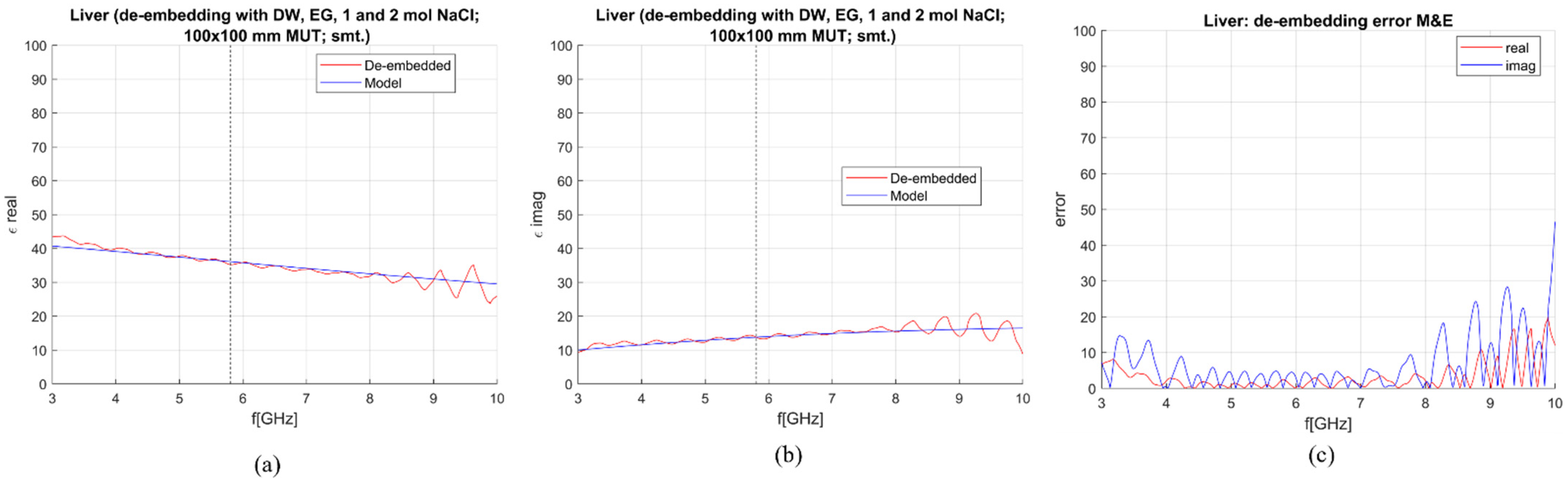
Figure 13.
M&E de-embedding with 2nd calibration option: DW, EG70, 1 mol and 2 mol NaCl (smoothing applied): (a) Calculated vs. reference ε′; (b) Calculated vs. reference ε″; (c) Sensitivity (de-embedding error) for ε′ (“real”) and ε″ (“imag”).
Figure 13.
M&E de-embedding with 2nd calibration option: DW, EG70, 1 mol and 2 mol NaCl (smoothing applied): (a) Calculated vs. reference ε′; (b) Calculated vs. reference ε″; (c) Sensitivity (de-embedding error) for ε′ (“real”) and ε″ (“imag”).
Figure 14.
M&E de-embedding with 3rd calibration option: DW, EG70, 0.1 mol and 2 mol NaCl (smoothing applied): (a) Calculated vs. reference ε′; (b) calculated vs. reference ε″; (c) sensitivity (de-embedding error) for ε′ (“real”) and ε″ (“imag”).
Figure 14.
M&E de-embedding with 3rd calibration option: DW, EG70, 0.1 mol and 2 mol NaCl (smoothing applied): (a) Calculated vs. reference ε′; (b) calculated vs. reference ε″; (c) sensitivity (de-embedding error) for ε′ (“real”) and ε″ (“imag”).
Figure 15.
(a) Reflection coefficient in dB simulated in livers of different sizes (all edge lengths); (b) Reflection coefficient differences between simulations performed in livers of different sizes (all edge lengths).
Figure 15.
(a) Reflection coefficient in dB simulated in livers of different sizes (all edge lengths); (b) Reflection coefficient differences between simulations performed in livers of different sizes (all edge lengths).
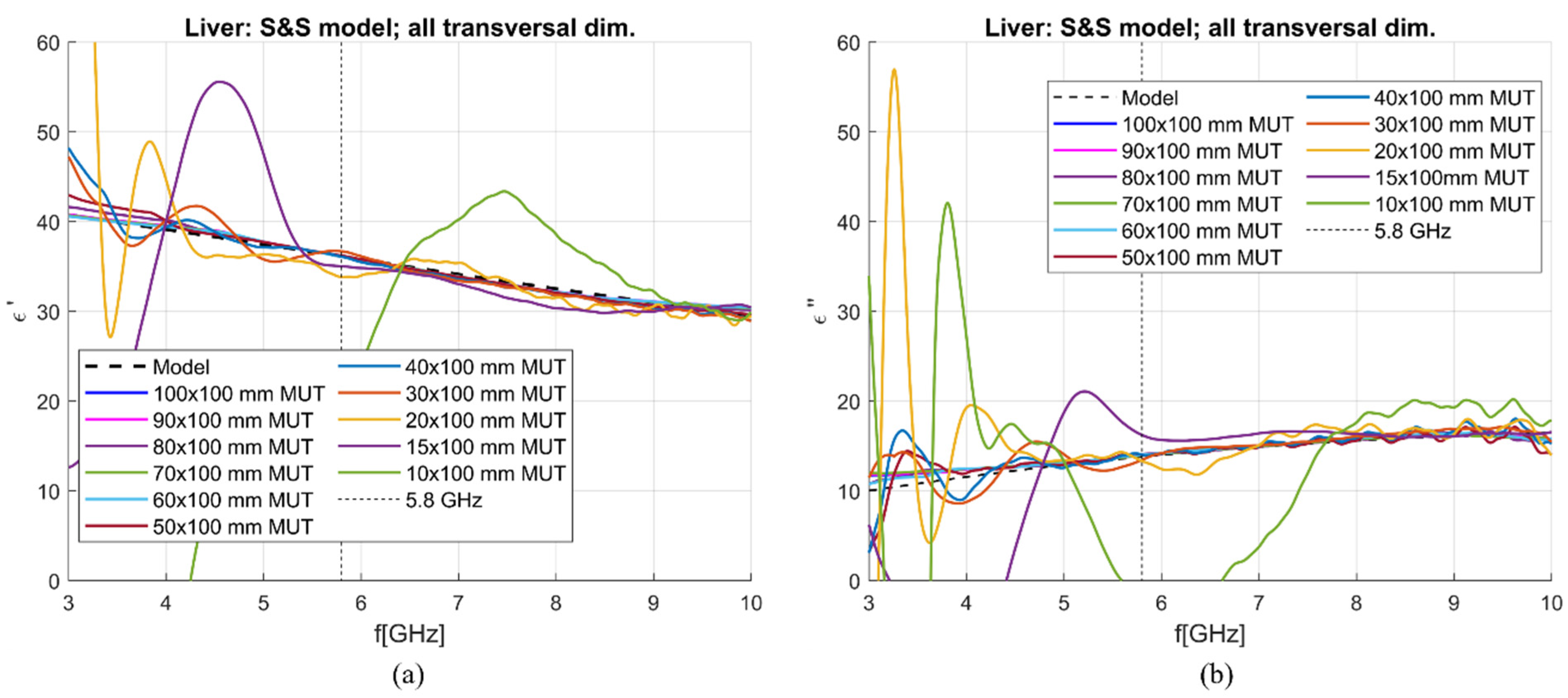
Figure 16.
S&S de-embedding of liver simulated in different blocks: (a) Calculated vs. reference ε′ (“real”); (b) calculated vs. reference ε″(“imag”).
Figure 16.
S&S de-embedding of liver simulated in different blocks: (a) Calculated vs. reference ε′ (“real”); (b) calculated vs. reference ε″(“imag”).
Figure 17.
Reflection coefficient in dB simulated in livers of different antenna tip—MUT bottom distances.
Figure 17.
Reflection coefficient in dB simulated in livers of different antenna tip—MUT bottom distances.
Figure 18.
S&S de-embedding of liver simulated in different blocks: (a) Calculated vs. reference ε′ (“real”); (b) calculated vs. reference ε″(“imag”).
Figure 18.
S&S de-embedding of liver simulated in different blocks: (a) Calculated vs. reference ε′ (“real”); (b) calculated vs. reference ε″(“imag”).
Figure 19.
S11 of the antenna immersed in the liver at different lengths.
Figure 19.
S11 of the antenna immersed in the liver at different lengths.
Figure 20.
S&S de-embedding of liver simulated with different antenna immersions: (a) real and (b) imaginary part of complex permittivity.
Figure 20.
S&S de-embedding of liver simulated with different antenna immersions: (a) real and (b) imaginary part of complex permittivity.
Table 1.
Design parameter overview.
Table 1.
Design parameter overview.
| Design Parameter | Parameter Value [mm] |
|---|
| Antenna: structure |
|
| 2 |
|
| 7.7 |
|
| 1.75 |
|
| 0.55 |
|
| 5.28 |
|
| 100 |
|
| 50 |
| Antenna: cross-section |
|
| 0.15 |
|
| 0.485 |
|
| 0.595 |
|
| 0.795 |
|
| 1.095 |
|
| 1.295 |
| MUT block (cube) |
| Cube edge | 100 |
Table 2.
1-pole Cole–Cole model parameters of simulated materials.
Table 2.
1-pole Cole–Cole model parameters of simulated materials.
| Material |
|
|
|
|
|
|---|
| Liver [15] | 44.32 | 5.32 | 11.55 | 0.25 | 36.115–j13.799 |
| DW at 25 °C [24] | 78.36 | 5.2 | 8.27 | / * | 72.268–j20.213 |
| 0.1 mol NaCl (at 20 °C) [25] | 78.1 | 5.22 | 9.1 | 0.96 | 70.879–j22.071 |
| 1 mol NaCl (at 20 °C) [21] | 67.9 | 5.22 | 8.53 | 7.81 | 62.377–j41.971 |
| 2 mol NaCl (at 20 °C) [21] | 59.4 | 5.22 | 8.13 | 13.29 | 55.028–j55.944 |
| EG70 (at 25 °C) [26] | 53.96 | 3.99 | 58.34 | / * | 19.175–j15.080 |
Table 3.
Averaged sensitivity in the 3–10 GHz range and at 5.8 GHz for S&S de-embedding with different calibration options.
Table 3.
Averaged sensitivity in the 3–10 GHz range and at 5.8 GHz for S&S de-embedding with different calibration options.
| | Measurement Sensitivity |
|---|
| | 3–10 GHz Range | @5.8 GHz |
|---|
| Calibration Option |
|
|
|
|
|---|
| OC, 0.1 mol and 2 mol NaCl | 13.15 | 40.59 | 6.61 | 32.30 |
| DW, 0.1 mol and 2 mol NaCl | 12.95 | 26.11 | 13.52 | 33.13 |
| DW, 1 mol and 2 mol NaCl | 15.44 | 33.84 | 7.57 | 23.22 |
| DW, 1 mol NaCl and EG70 | 0.85 | 3.09 | 0.07 | 1.09 |
Table 4.
Averaged sensitivity in the 3–10 GHz range and at the operating frequency for M&E de-embedding with different calibration options.
Table 4.
Averaged sensitivity in the 3–10 GHz range and at the operating frequency for M&E de-embedding with different calibration options.
| | Measurement Sensitivity |
|---|
| | In the 3–10 GHz Range | At 5.8 GHz |
|---|
| Calibration Option |
|
|
|
|
|---|
| OC, DW, 0.1 mol and 2 mol NaCl | 12.75 | 20.70 | 13.35 | 11.52 |
| DW, EG70, 1 mol and 2 mol NaCl | 3.28 | 6.61 | 2.46 | 0.14 |
| DW, EG70, 0.1 mol and 2 mol NaCl | 1.48 | 6.57 | 1.42 | 3.20 |
Table 5.
Average sensitivity in the 5–6 GHz range and at 5.8 GHz for different sizes of MUT.
Table 5.
Average sensitivity in the 5–6 GHz range and at 5.8 GHz for different sizes of MUT.
| | Measurement Sensitivity | |
|---|
| | In the 5–6 GHz Range | At 5.8 GHz |
|---|
|
|
|
|
|
|
|---|
| 100 × 100 | 0.29 | 1.33 | 0.07 | 1.09 |
| 90 × 100 | 0.30 | 1.26 | 0.04 | 1.02 |
| 80 × 100 | 0.08 | 1.85 | 0.29 | 1.42 |
| 70 × 100 | 0.28 | 1.34 | 0.06 | 1.02 |
| 60 × 100 | 0.28 | 1.46 | 0.10 | 1.56 |
| 50 × 100 | 0.39 | 1.38 | 0.26 | 1.39 |
| 40 × 100 | 0.33 | 1.48 | 0.10 | 1.50 |
| 30 × 100 | 2.13 | 4.74 | 1.56 | 2.55 |
| 20 × 100 | 4.28 | 4.48 | 6.36 | 3.46 |
| 15 × 100 | 6.17 | 37.37 | 3.04 | 17.55 |
| 10 × 100 | 58.22 | 79.88 | 45.76 | 121.88 |
Table 6.
Average sensitivity in the 5–6 GHz range and at 5.8 GHz for different immersion lengths.
Table 6.
Average sensitivity in the 5–6 GHz range and at 5.8 GHz for different immersion lengths.
| | Measurement Sensitivity | |
|---|
| | In the 5–6 GHz Range | At 5.8 GHz |
|---|
| Antenna Immersion [mm] |
|
|
|
|
|---|
| 50 | 0.29 | 1.33 | 0.07 | 1.09 |
| 45 | 2.00 | 7.89 | 1.61 | 7.06 |
| 40 | 1.55 | 7.33 | 1.66 | 8.64 |
| 30 | 5.57 | 17.21 | 0.66 | 20.08 |
| 20 | 24.98 | 20.15 | 7.81 | 21.97 |


