
A Condition Evaluation Simplified Method for Traction Converter Power Module Based on Operating Interval Segmentation

Abstract
:1. Introduction
2. Digital Simulation Model of Power Module
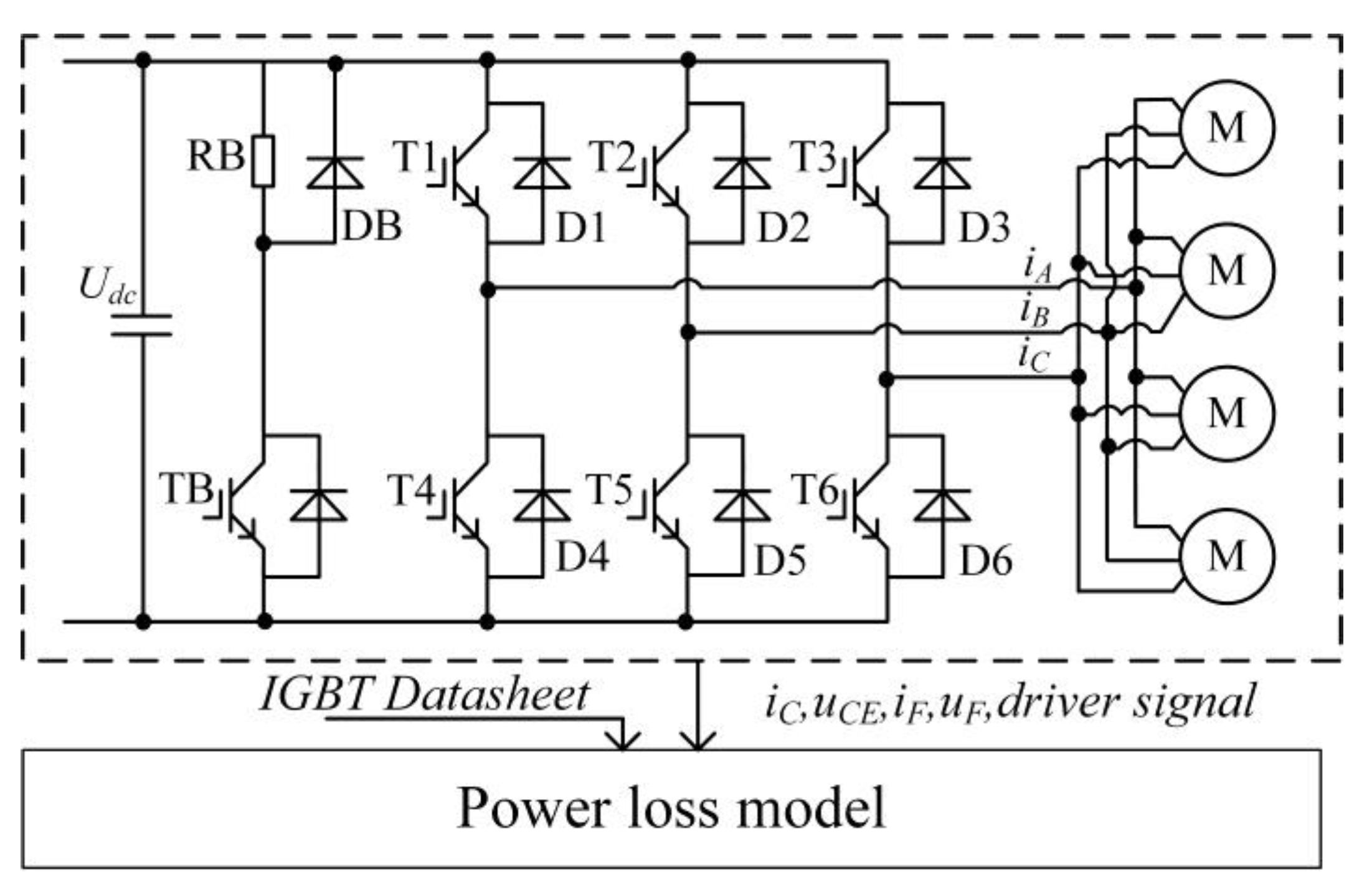
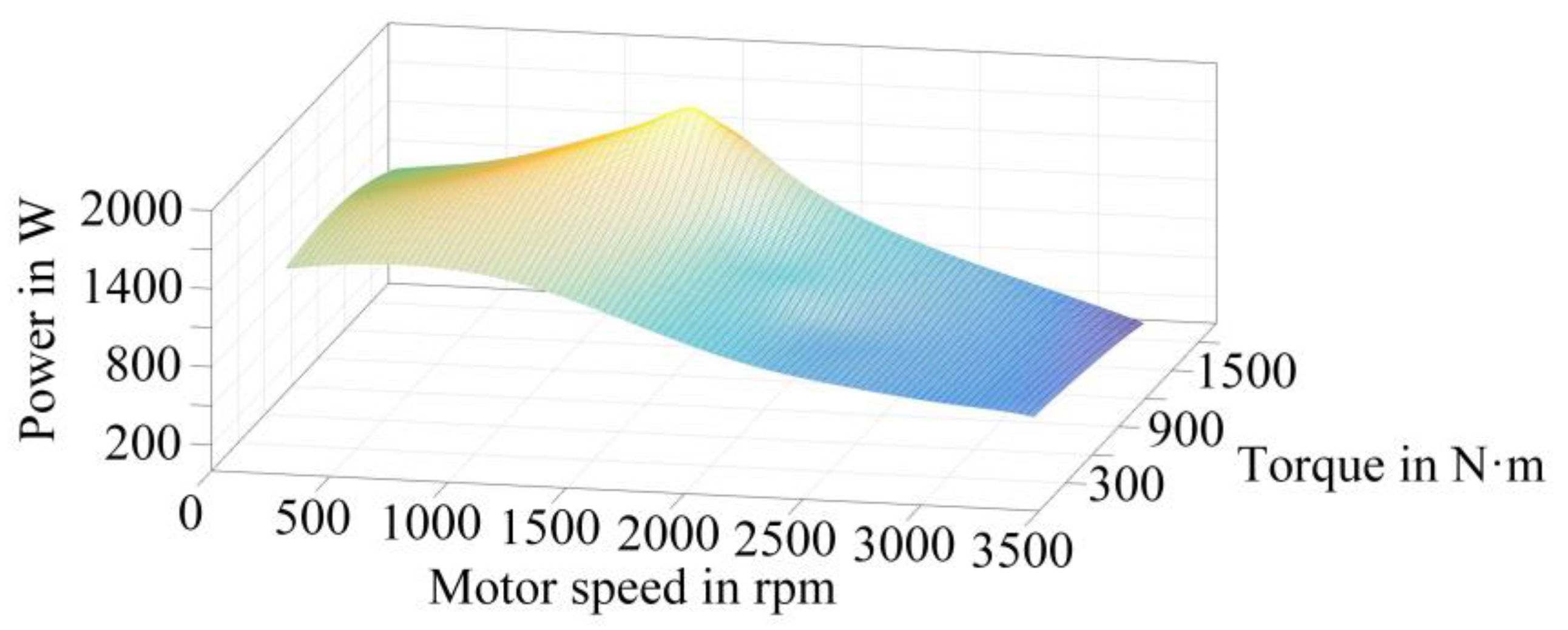
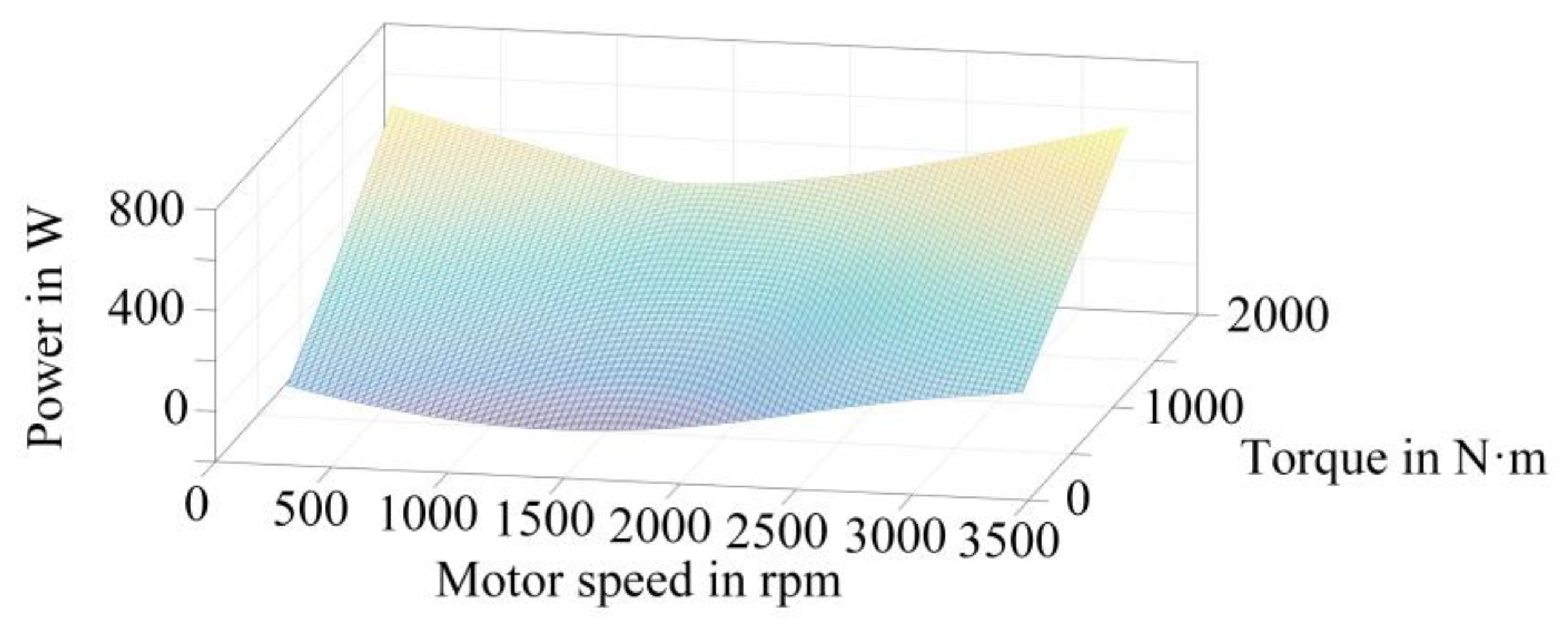
2.1. Power Loss Model of Power Module
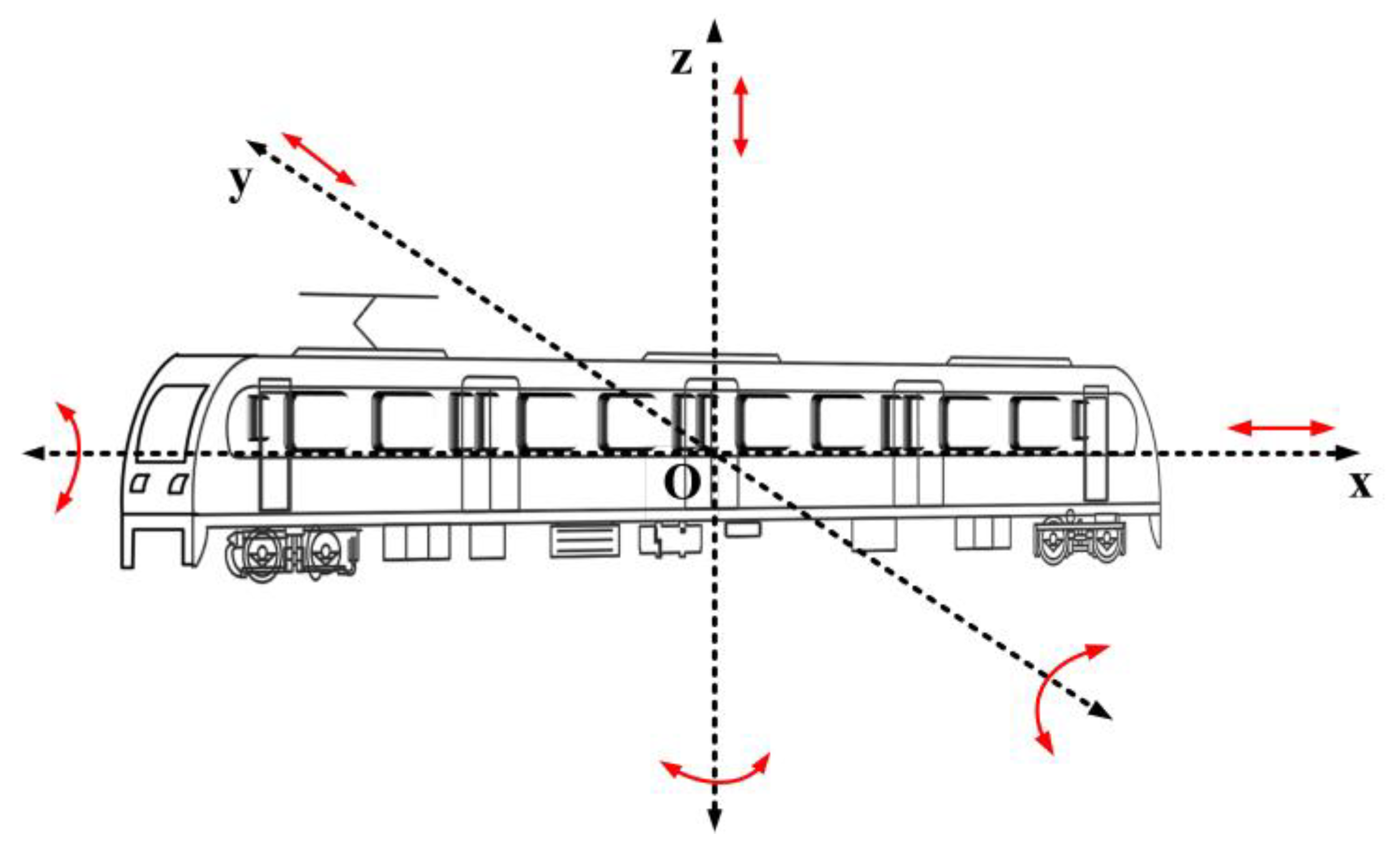
2.2. Random Vibration Analysis
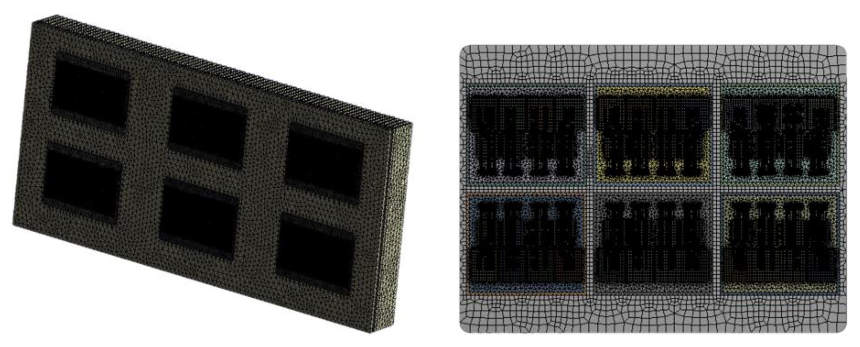
2.3. Finite Element Simulation Model
3. Condition Evaluation Simplified Simulation Method Based on OIS
3.1. Method Introduction
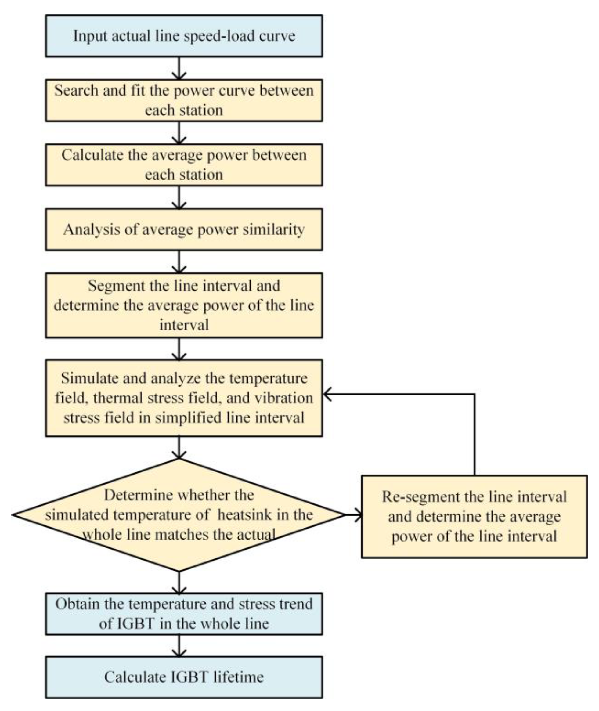
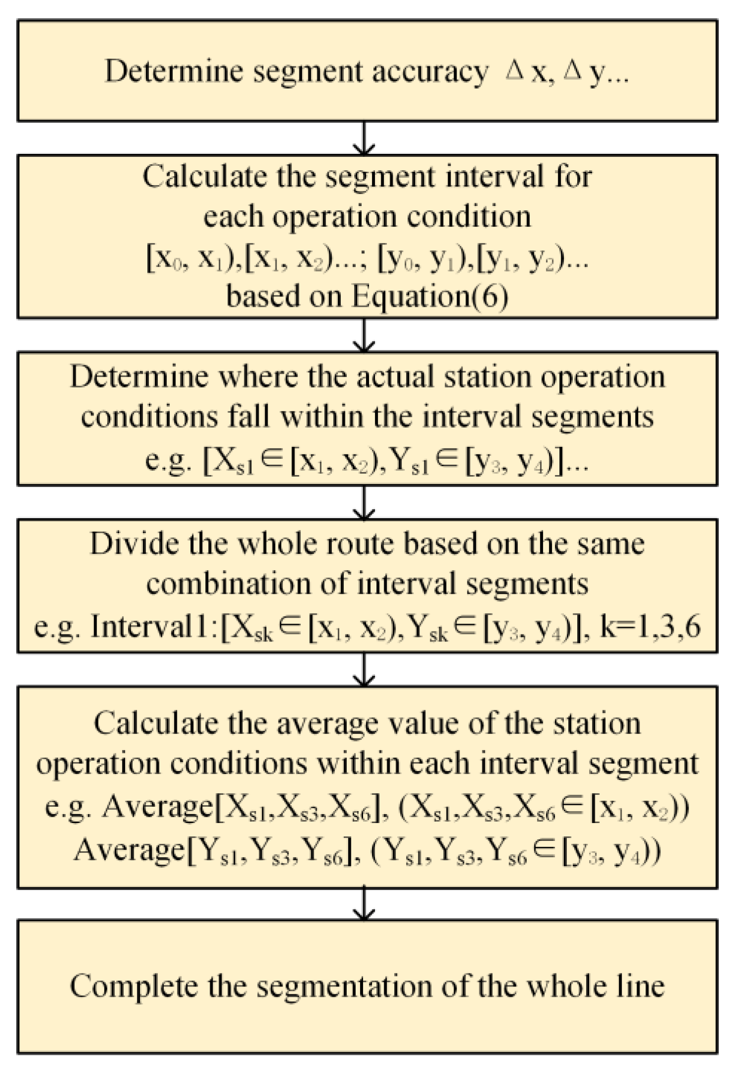
3.1.1. Flow Chart of Simplified Condition Evaluation Based on OIS
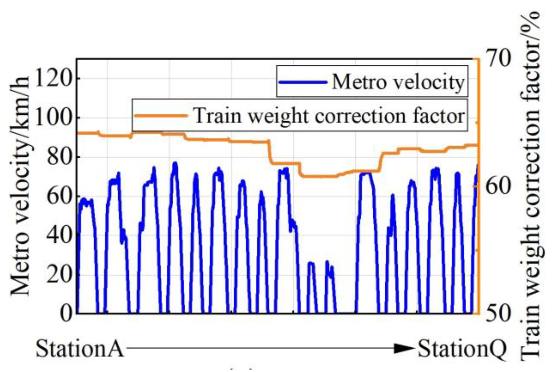
3.1.2. OIS Mathematical Model with a Flow Chart
3.2. Simulation and Analysis Process
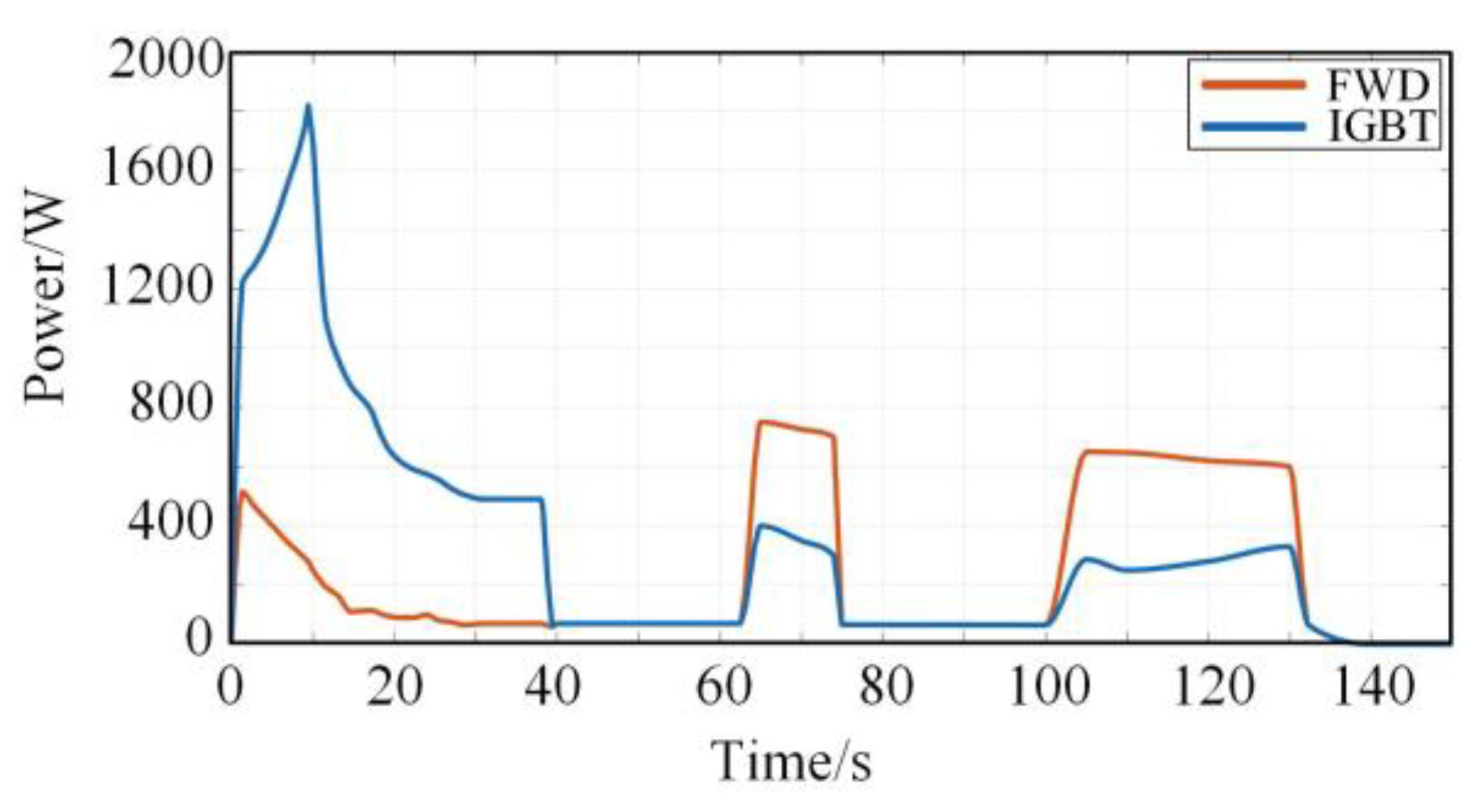
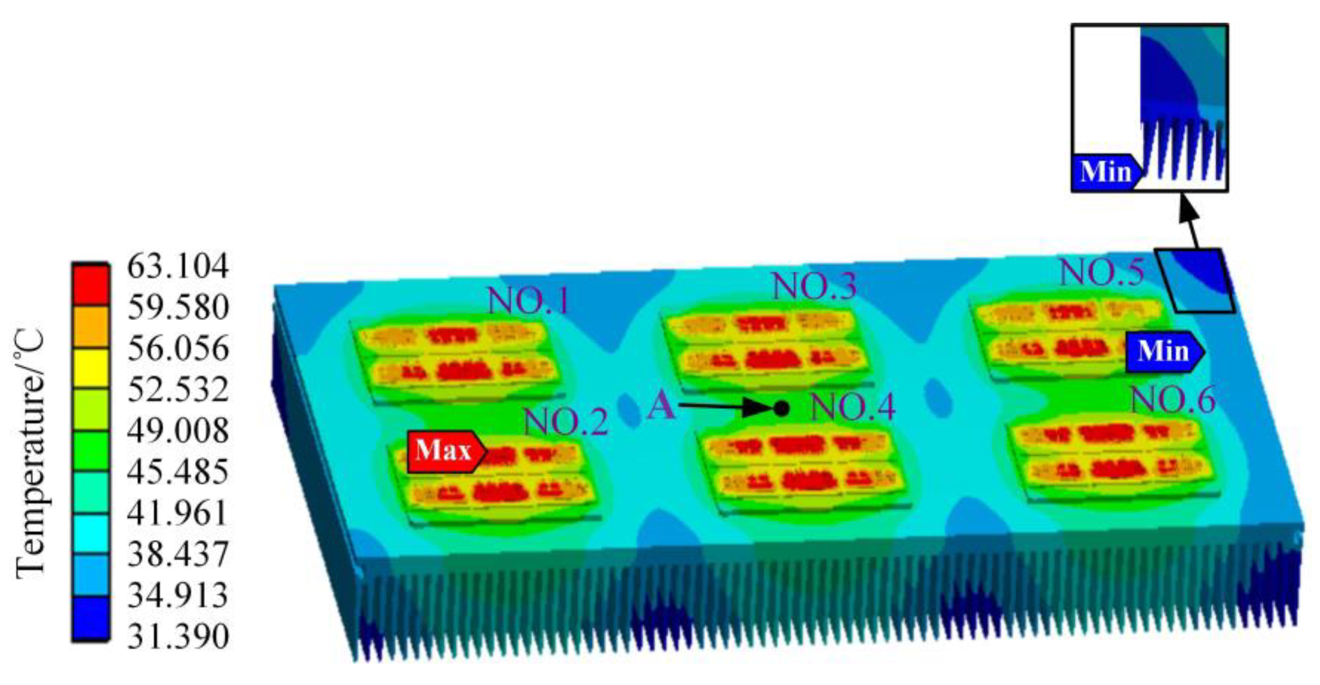
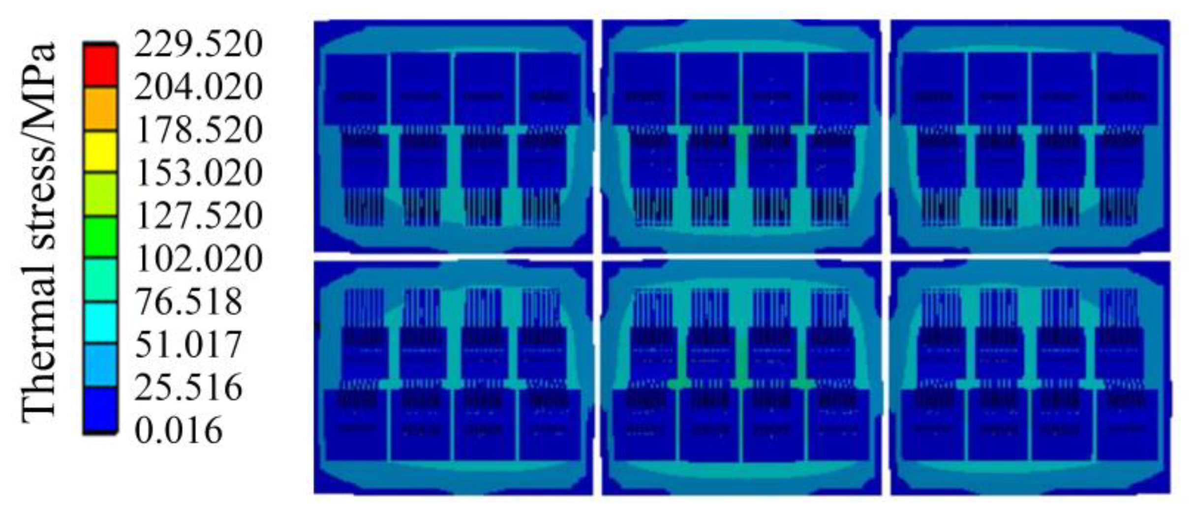
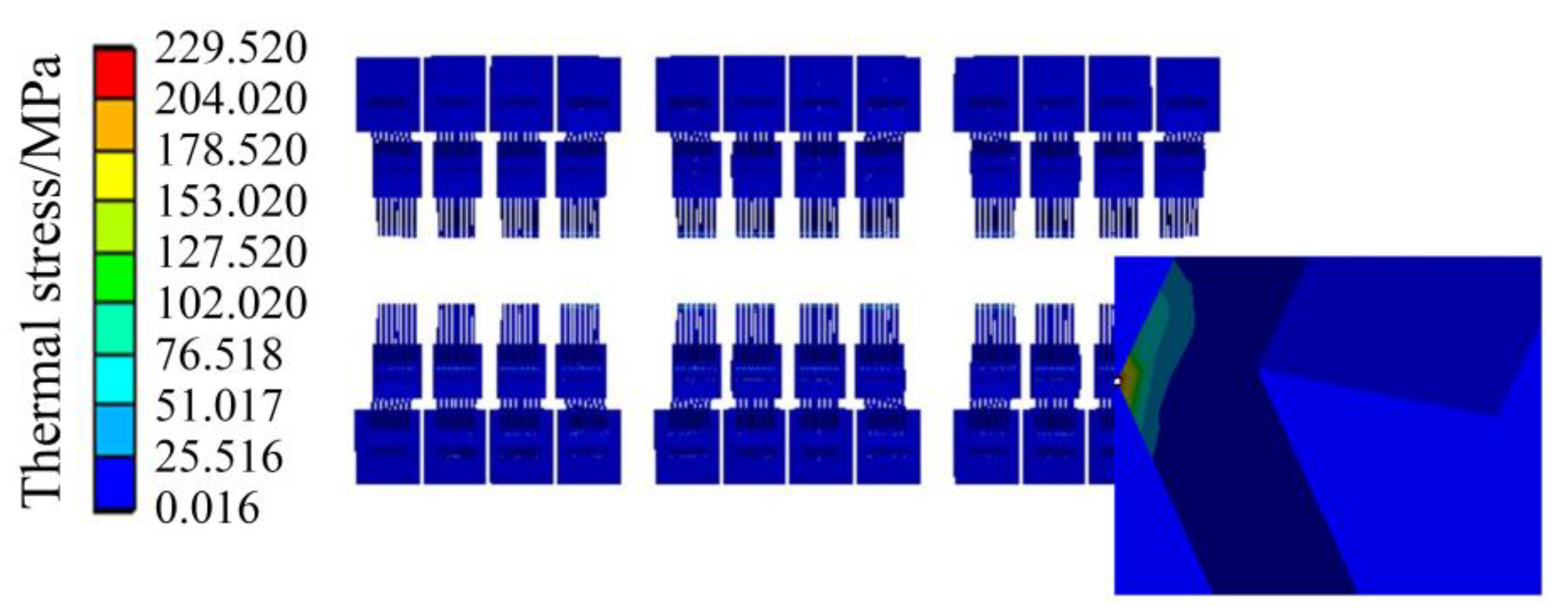
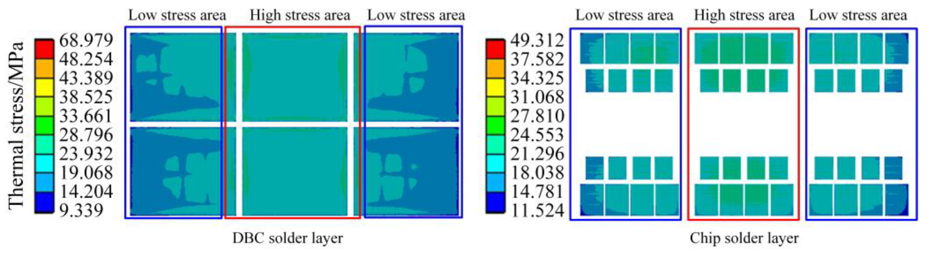
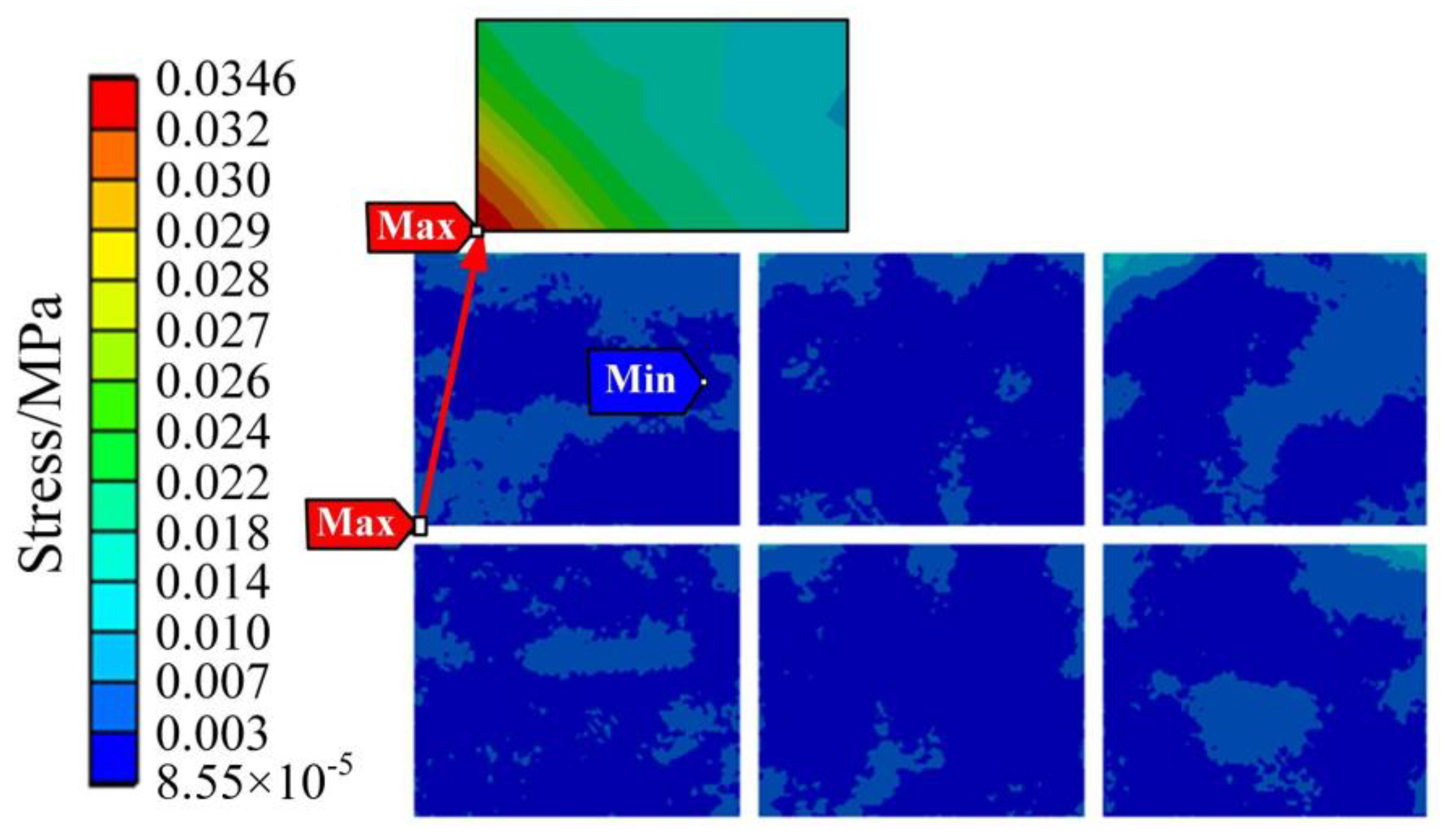
3.2.1. Simulation of Temperature Field and Thermal Stress
3.2.2. Modal Analysis of IGBT Module
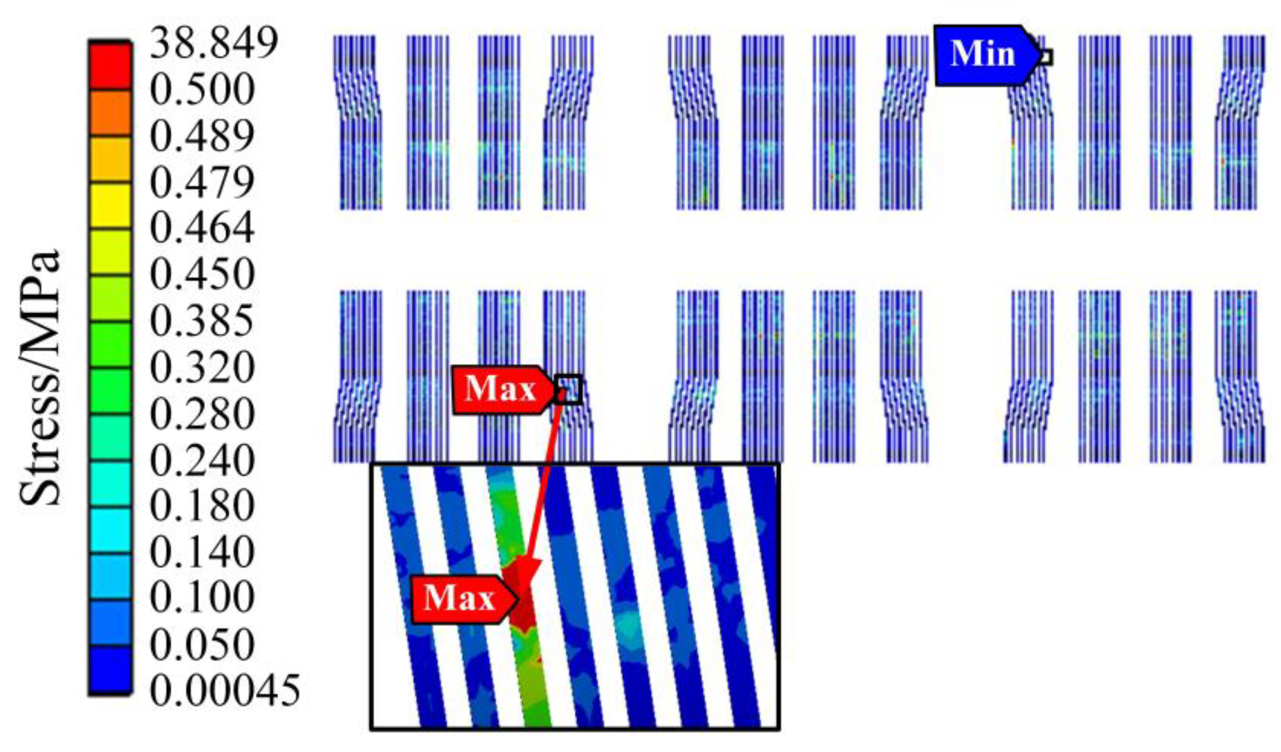
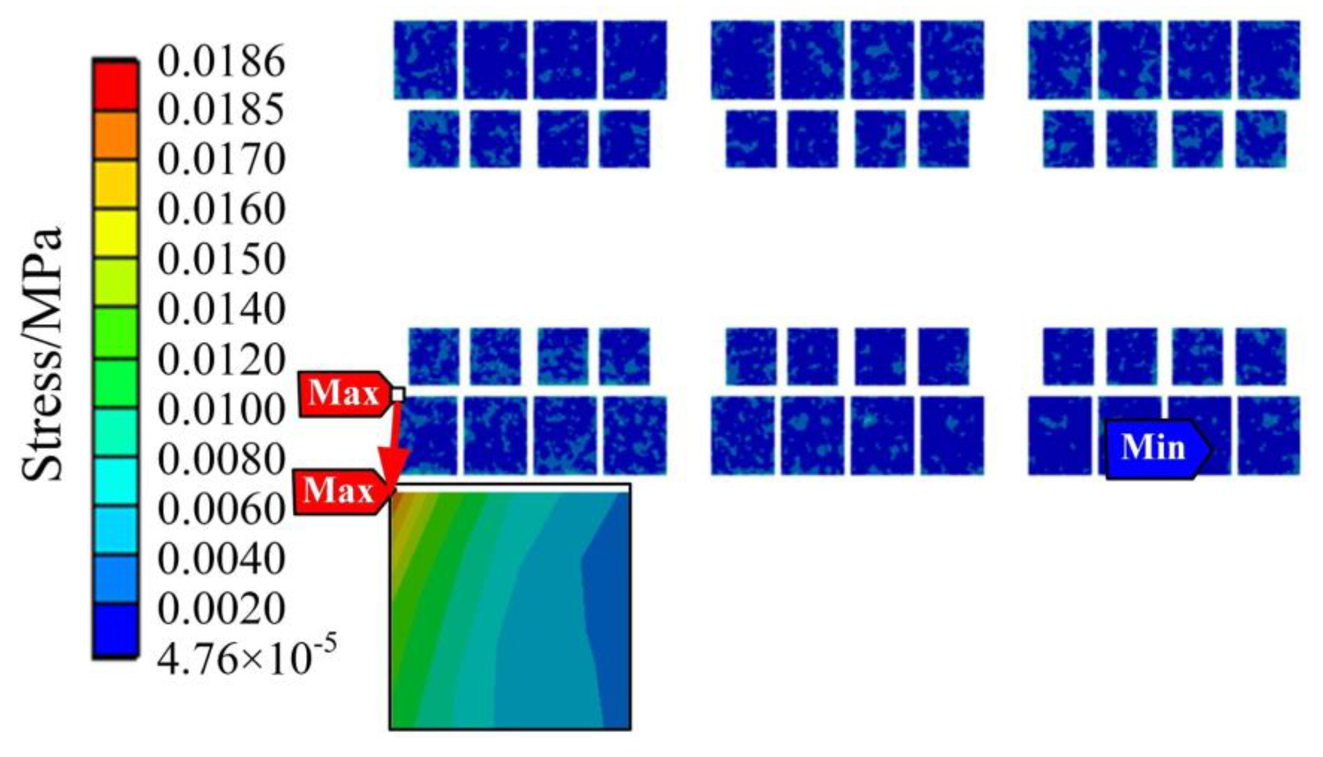
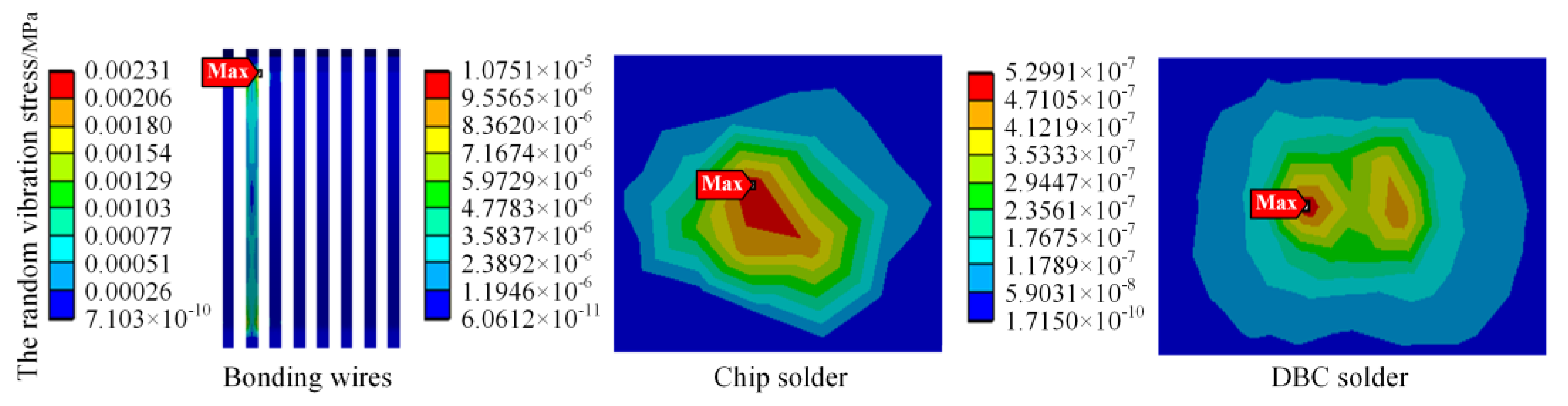
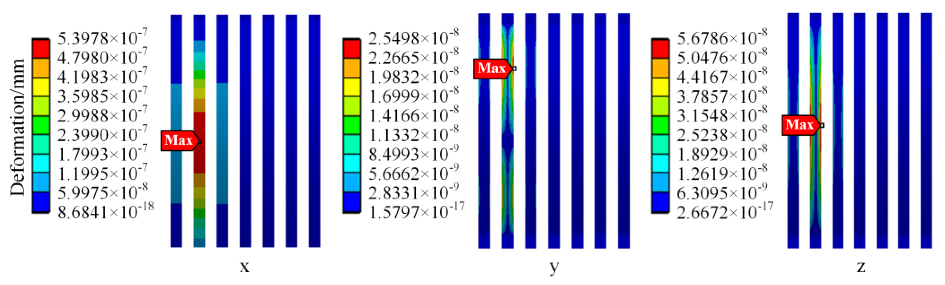
3.2.3. Vibration Stress Simulation
4. Method Validation
4.1. Method Accuracy and Efficiency Validation
4.2. Method Application
5. Conclusions
Author Contributions
Funding
Institutional Review Board Statement
Informed Consent Statement
Data Availability Statement
Acknowledgments
Conflicts of Interest
References
- Dong, H.; Chen, F.; Wang, Z.; Jia, L.; Qin, Y.; Man, J. An Adaptive Multisensor Fault Diagnosis Method for High-Speed Train Traction Converters. IEEE Trans. Power Electron. 2021, 36, 6288–6302. [Google Scholar] [CrossRef]
- Ge, X.; Xie, D.; Deng, Q. Overview of Fault Diagnosis and Fault-tolerant Control Methods for Vehicular Traction Converter System. J. Power Supply 2020, 18, 28–44. [Google Scholar]
- Ahsan, M.; Hon, S.T.; Batunlu, C.; Albarbar, A. Reliability Assessment of IGBT Through Modelling and Experimental Testing. IEEE Access 2020, 8, 39561–39573. [Google Scholar] [CrossRef]
- Ma, K.; Xu, M.; Liu, B. Modeling and Characterization of Frequency-Domain Thermal Impedance for IGBT Module Through Heat Flow Information. IEEE Trans. Power Electron. 2021, 36, 1330–1340. [Google Scholar] [CrossRef]
- Luo, D.; Chen, M.; Lai, W.; Xia, H.; Li, H.; Yu, K. A Fault Detection Method for Partial Chip Failure in Multichip IGBT Modules Based on Turn-Off Delay Time. IEEE Trans. Electron Devices 2022, 69, 3319–3327. [Google Scholar] [CrossRef]
- Wang, K.; Zhou, L.; Sun, P.; Du, X. Monitoring Bond Wires Fatigue of Multichip IGBT Module Using Time Duration of the Gate Charge. IEEE Trans. Power Electron. 2021, 36, 888–897. [Google Scholar] [CrossRef]
- Wang, H.; Liu, D.; Fan, Y.; Wu, Y.; Qiao, T.; Yang, D.G. Modal Analysis of IGBT Power Devices Based on ANSYS. In Proceedings of the 2019 20th International Conference on Electronic Packaging Technology (ICEPT), Hong Kong, China, 12–15 August 2019. [Google Scholar]
- Gonzalez-Hernando, F.; San-Sebastian, J.; Arias, M.; Rujas, A.; Mir, L. Active Thermal Control for Lifetime Extension of Traction Converter. In Proceedings of the 10th International Conference on Power Electronics Machines and Drives (PEMD 2020), Online Conference, 15–17 December 2020. [Google Scholar]
- Ke, Q.; Xu, Z.; Ge, X.; Deng, Q.; Wang, H.; Zhang, L.; Li, J. Mission-Profile Based Reliability Analysis Scheme of IGBT Modules for Traction Rectifier. In Proceedings of the 2022 International Power Electronics Conference (IPEC-Himeji 2022-ECCE Asia), Himeji, Japan, 15–19 May 2022. [Google Scholar]
- Tang, Y.; Wang, B.; Chen, M.; Liu, B. Reliability and On-Line Evaluation of IGBT Modules Under High Temperature. Trans. China Electrotech. Soc. 2014, 29, 17–23. [Google Scholar]
- Liu, X.; Sooklal, V.K.; Verges, M.A.; Larson, M.C. Experimental Study and Life Prediction on High Cycle Vibration Fatigue in BGA Packages. Microelectron. Reliab. 2006, 46, 1128–1138. [Google Scholar] [CrossRef]
- Kim, Y.; Noguchi, H.; Amagai, M. Vibration Fatigue Reliability of BGA-IC Package with Pb-free Solder and Pb-Sn Solder. Microelectron. Reliab. 2006, 46, 459–466. [Google Scholar] [CrossRef]
- Huang, T. The Research on Wheel and Track Vibration and Noise Radiation. Master’s Thesis, Shanghai Jiaotong University, Shanghai, China, 2007. [Google Scholar]
- Wang, H.; Zhao, M.; Chen, Y. Vibration Fatigue Life Prediction Model for Flip Chip Solder Joint. J. Shanghai Jiaotong Univ. 2001, 12, 1855–1857. [Google Scholar]
- Huang, X.; Tian, D.; Wang, F.; Chen, C.; Sun, H. Mission Profiles-Based Lifetime Prediction for IGBT Modules Applied to CRH3 Traction Converter. Trans. China Electrotech. Soc. 2022, 37, 172–180. [Google Scholar]
- Xia, H.; Zhang, Y.; Zhou, D.; Chen, M.; Lai, W.; Wei, Y.; Wang, H. Impact of Loss Model Selection on Power Semiconductor Lifetime Prediction in Electric Vehicles. In Proceedings of the IECON 2022-48th Annual Conference of the IEEE Industrial Electronics Society, Brussels, Belgium, 17–20 October 2022. [Google Scholar]
- Lin, S.; Fang, X.; Li, B.; Lin, F.; Yang, Z. Reliability-Oriented Control Strategy of Traction Converters in Urban Rail Transit Trains. Trans. China Electrotech. Soc. 2022, 36, 704–712. [Google Scholar]
- Wang, X.; Zhu, C.; Luo, H.; Lu, Z.; Li, W.; He, X.; Ma, J.; Chen, G.; Tian, Y.; Yang, E. IGBT Junction Temperature Measurement Via Combined TSEPs With Collector Current Impact Elimination. In Proceedings of the 2016 IEEE Energy Conversion Congress and Exposition (ECCE), Milwaukee, WI, USA, 18–22 September 2016. [Google Scholar]
- Warwel, M.; Wittler, G.; Hirsch, M.; Reuss, H.-C. Real-time Thermal Monitoring of Power Semiconductors in Power Electronics Using Linear Parameter-varying Models for Variable Coolant Flow Situations. In Proceedings of the 2014 IEEE 15th Workshop on Control and Modeling for Power Electronics (COMPEL), Santander, Spain, 22–25 June 2014. [Google Scholar]
- Zhou, J.; Li, B.; He, Y.; Yuan, W.; Liu, J.; Ni, H. Electro-Thermal-Mechanical Multiphysics Coupling Failure Analysis Based on Improved IGBT Dynamic Model. IEEE Access 2019, 7, 174155–174166. [Google Scholar] [CrossRef]
- Dai, S.; Wang, Z.; Wu, H.; Song, X.; Li, G.; Pickert, V. Thermal and Mechanical Analyses of Clamping Area on the Performance of Press-Pack IGBT in Series-Connection Stack Application. IEEE Trans. Compon. Packag. Manuf. Technol. 2021, 11, 200–211. [Google Scholar] [CrossRef]
- Wang, J.; Chen, W.; Wang, L.; Wang, B.; Zhao, C.; Ma, D.; Yang, F.; Li, Y. A Transient 3-D Thermal Modeling Method for IGBT Modules Considering Uneven Power Losses and Cooling Conditions. IEEE J. Emerg. Sel. Top. Power Electron. 2021, 9, 3959–3970. [Google Scholar] [CrossRef]
- Zhang, J.; Zhang, L.; Cheng, Y. Review of the Lifetime Evaluation for the IGBT Module. Trans. China Electrotech. Soc. 2021, 12, 2560–2575. [Google Scholar]
- Lu, Y.; Yang, L.; Meng, F.; Xia, D.; Qi, J. Collaborative Optimization of Train Timetable and Passenger Flow Control Strategy for Urban Rail Transit. J. Transp. Syst. Eng. Inf. Technol. 2021, 21, 195–202. [Google Scholar]
- Li, W. Study on vibration characteristics and active vibration reduction of traction transmission system of high speed train. Master’s Thesis, Chongqing University, Chongqing, China, 2021. [Google Scholar]
- Tsunashima, H. Condition Monitoring of Railway Tracks from Car-Body Vibration Using a Machine Learning Technique. Appl. Sci. 2019, 9, 2734–2746. [Google Scholar] [CrossRef] [Green Version]
- Wang, H. Failure Analysis of Power Device IGBT under High Temperature Vibration Condition. Master’s Thesis, Guilin University of Electronic Technology, Guilin, China, 2021. [Google Scholar]
- Lin, S.; Fang, X.; Lin, F.; Yang, Z. Mission Profiles-based Lifetime Prediction for IGBT Modules in Traction Inverter Application. China Saf. Sci. J. 2019, 29, 52–57. [Google Scholar]
- Morozumi, A.; Yamada, K.; Miyasaka, T.; Sumi, S.; Seki, Y. Reliability of power cycling for IGBT power semiconductor modules. IEEE Trans. Ind. Appl. 2003, 39, 665–671. [Google Scholar] [CrossRef]
- Zeng, W. Study on Stress Characteristics and Fatigue Life of Subway Bogie Frame under Random Vibration. Master’s Thesis, Beijing Jiaotong University, Beijing, China, 2019. [Google Scholar]
- Wang, L.; Xu, W.; Liu, S.; Qiu, R.; Xu, C. Online Fatigue Estimation and Prediction of Switching Device in Urban Railway Traction Converter Based on Current Recognition and Gray Model. IEEE Access 2019, 7, 123307–123319. [Google Scholar] [CrossRef]
- Wang, J.; Chen, W.; Wu, Y.; Zhang, J.; Wang, L.; Liu, J. Chip-Level Electrothermal Stress Calculation Method of High-Power IGBT Modules in System-Level Simulation. IEEE Trans. Power Electron. 2022, 37, 10546–10561. [Google Scholar] [CrossRef]
- Li, H.; Lai, W.; Li, H.; Yao, R.; Yu, K.A. Research on solder layer void evolution mechanism for IGBT module of electric locomotive in service. Electr. Drive Locomot. 2022, 6, 138–148. [Google Scholar]
- Dauksher, W. A Second-Level SAC Solder-Joint Fatigue-Life Prediction Methodology. IEEE Trans. Device Mater. Reliab. 2008, 8, 168–173. [Google Scholar] [CrossRef]
- Morrow, J. ASTM STP 378; Cyclic Plastic Strain Energy and Fatigue of Metals. American Society for Testing and Materials: West Conshohocken, PA, USA, 1964. [Google Scholar]


| Frequency (Hz) | PSD Grade (g2/Hz) |
|---|---|
| 5 | 0.00002 |
| 17 | 0.001 |
| 40 | 0.001 |
| 50 | 0.01 |
| 60 | 0.01 |
| 70 | 0.001 |
| 150 | 0.001 |
| 200 | 0.0005 |
| 500 | 0.0005 |
| Internal Unit | Material Composition | Dimension (mm) |
|---|---|---|
| Bonding wire | Ag | 0.4 (diameter) 1.3 (arc height) |
| IGBT chip | Si | 15 × 12.5 × 0.45 |
| FWD chip | Si | 11 × 9.8 × 0.45 |
| Solder layer 1 | SnAg | 15 × 12.5 × 0.1 (IGBT) 11 × 9.8 × 0.1 (FWD) |
| Copper layer 1 | Cu | 55 × 46 × 0.3 |
| Liners | AlN | 58 × 49 × 0.8 |
| Copper layer 2 | Cu | 58 × 49 × 0.3 |
| Solder layer 2 | SnAg | 58 × 49 × 0.4 |
| Substrate | Al-SiC | 187.5 × 137 × 4.7 |
| Length | Width | Substrate Thickness | Tooth Length | Tooth Thickness | Tooth Pitch |
|---|---|---|---|---|---|
| 920 | 450 | 16 | 72 | 3.36 | 12 |
| Layer | Density (kg·m−3) | Thermal Conductivity (W·(m·K)−1) | Coefficient of Thermal Expansion (10−6·K−1) | Specific Heat Capacity (J·(kg·K)−1) | Elastic Modulus (GPa) | Poisson’s Ratio |
|---|---|---|---|---|---|---|
| Bonding wire | 11,000 | 429 | 19 | 232 | 83 | 0.37 |
| Chip layer | 2330 | 118 | 2.9 | 690 | 130 | 0.28 |
| Solder layer | 7360 | 33 | 30 | 180 | 13.8 | 0.35 |
| Copper layer | 5361 | 200 | 7.4 | 519 | 225 | 0.29 |
| Substrate | 2960 | 220 | 7.9 | 741 | 741 | 0.22 |
| Liner | 3220 | 150 | 3.5 | 740 | 325 | 0.31 |
| Heat-sink | 2689 | 273.5 | 23 | 951 | 71 | 0.33 |
| Orders | Frequency (Hz) |
|---|---|
| 1 | 0 |
| 2 | 0 |
| 3 | 0 |
| 4 | 0.0015 |
| 5 | 0.0092963 |
| 6 | 0.011533 |
| 7 | 1985.8 |
| 8 | 2130.3 |
| 9 | 4454 |
| 10 | 4568.6 |
| 11 | 5609.8 |
| Orders | Frequency (Hz) |
|---|---|
| 1 | 8639 |
| 2 | 8639 |
| 3 | 8639.8 |
| 4 | 8639.9 |
| 5 | 8640 |
| 6 | 8640.2 |
| 7 | 8640.4 |
| 8 | 8640.4 |
| 9 | 8640.5 |
| 10 | 8640.8 |
| 11 | 8640.9 |
| Parameter | Value |
|---|---|
| DC Voltage | 1.5 kV |
| DC-link capacitor in a converter | 4300 μF |
| IGBT | FZ1500R33HE3 |
| Switch frequency | 450 Hz |
| Traction motor nominal/maximum current | 132 A/271 A |
| Traction motor nominal power | 210 kW |
| Traction motor nominal/maximum speed | 1800 rpm/3472 rpm |
| Traction motor maximum traction force | 1630 Nm |
| Traction motor nominal displacement factor | 0.85 |
| Cooling system | Forced air cooling |
| Oscilloscope | DL750 |
| Chopper diode | FZ1500R33HE3 |
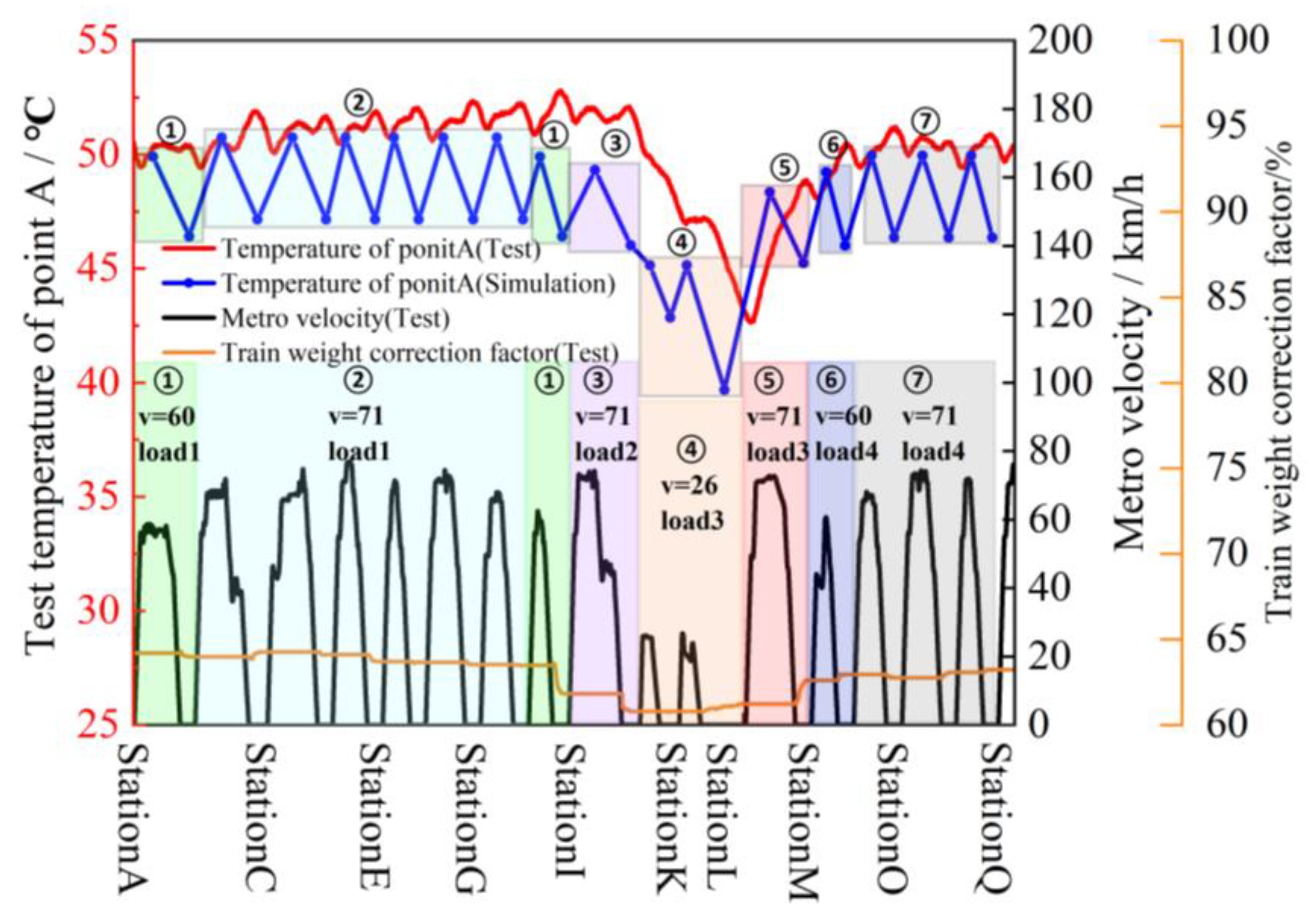
| Interval | Interval1 | Interval2 | Interval3 | Interval4 | Interval5 | Interval6 | Interval7 |
|---|---|---|---|---|---|---|---|
| Velocity | 60 | 71 | 71 | 26 | 71 | 60 | 71 |
| Load | 63.87% | 63.87% | 61.83% | 60.9% | 60.9% | 62.85% | 62.85% |
Disclaimer/Publisher’s Note: The statements, opinions and data contained in all publications are solely those of the individual author(s) and contributor(s) and not of MDPI and/or the editor(s). MDPI and/or the editor(s) disclaim responsibility for any injury to people or property resulting from any ideas, methods, instructions or products referred to in the content. |
© 2023 by the authors. Licensee MDPI, Basel, Switzerland. This article is an open access article distributed under the terms and conditions of the Creative Commons Attribution (CC BY) license (https://creativecommons.org/licenses/by/4.0/).
Share and Cite
Wang, L.; Zhou, M.; Dongye, Z.; Sha, Y.; Chen, J. A Condition Evaluation Simplified Method for Traction Converter Power Module Based on Operating Interval Segmentation. Sensors 2023, 23, 2537. https://doi.org/10.3390/s23052537
Wang L, Zhou M, Dongye Z, Sha Y, Chen J. A Condition Evaluation Simplified Method for Traction Converter Power Module Based on Operating Interval Segmentation. Sensors. 2023; 23(5):2537. https://doi.org/10.3390/s23052537
Chicago/Turabian StyleWang, Lei, Mingchao Zhou, Zhonghao Dongye, Yanbei Sha, and Jingcao Chen. 2023. "A Condition Evaluation Simplified Method for Traction Converter Power Module Based on Operating Interval Segmentation" Sensors 23, no. 5: 2537. https://doi.org/10.3390/s23052537