
Research on Anomaly Detection of Surveillance Video Based on Branch-Fusion Net and CSAM
Abstract
:1. Introduction
- (1)
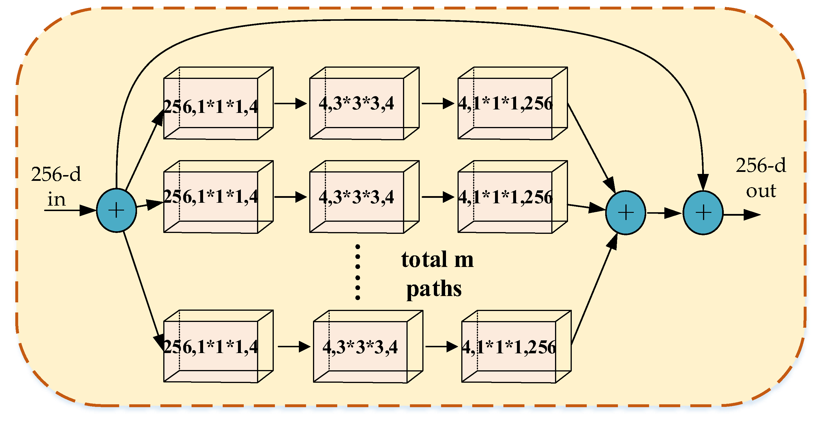
- We propose the Branch-Fusion Net, which not only greatly reduces parameter overhead, but also improves the generalization ability of feature extraction by understanding the input feature maps from multiple perspectives. The network achieves state-of-the-art performance for behavior recognition tasks on multiple benchmarks.
- (2)
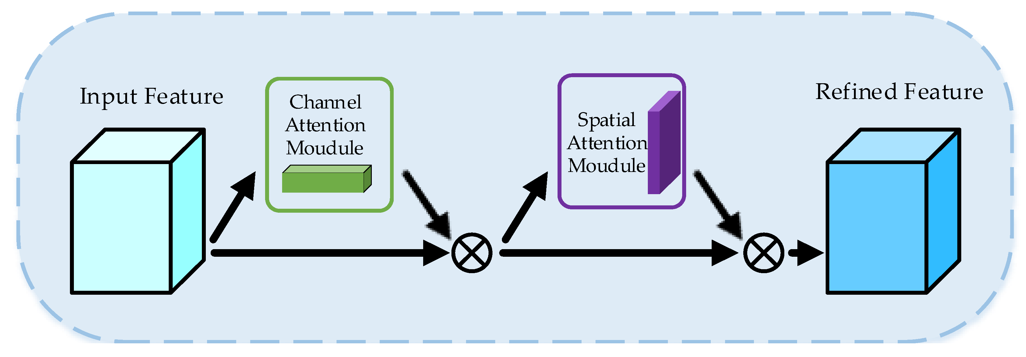
- We propose a simple yet effective CSAM to ignore useless features during the model training. The CSAM focuses attention on key channels and spatial feature areas in turn. Adding the CSAM to the mainstream 3D convolutional neural networks can significantly improve the feature extraction effect.
- (3)
- We establish a surveillance video dataset called ‘Crimes-mini’ containing five categories of abnormal behaviors. The model we propose achieves the detection accuracy of 93.55% on the test set.
2. Related Work
2.1. Anomaly Detection Methods
2.2. Feature Extraction Network for Video
3. The Network Architecture
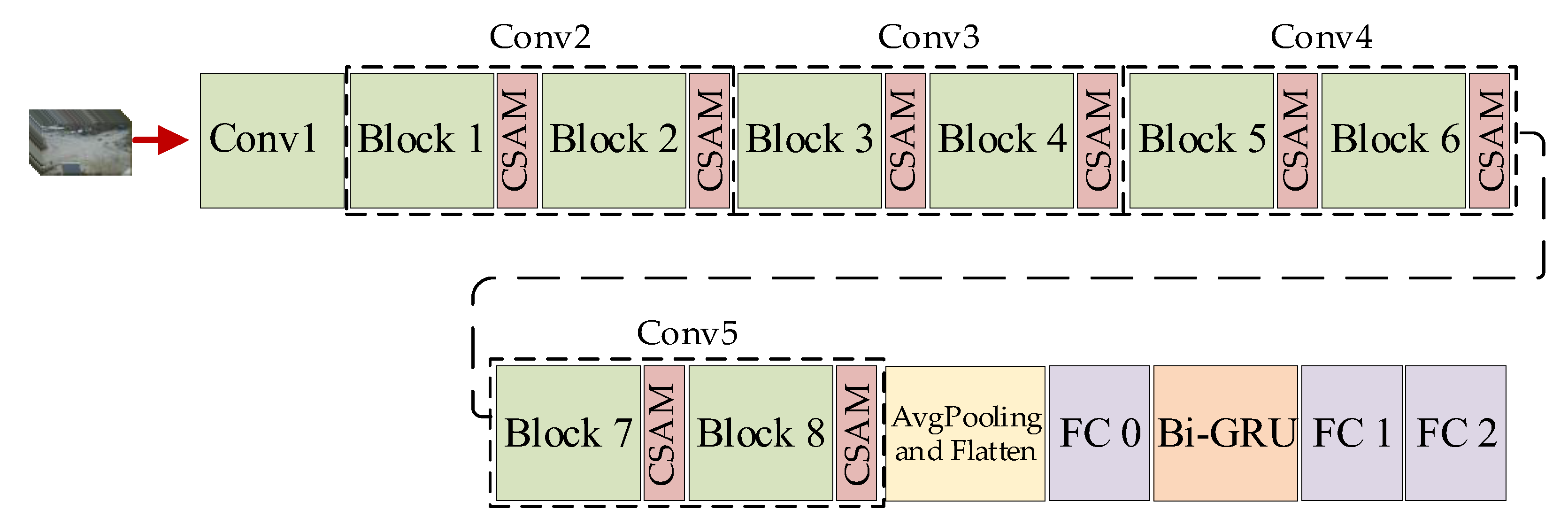
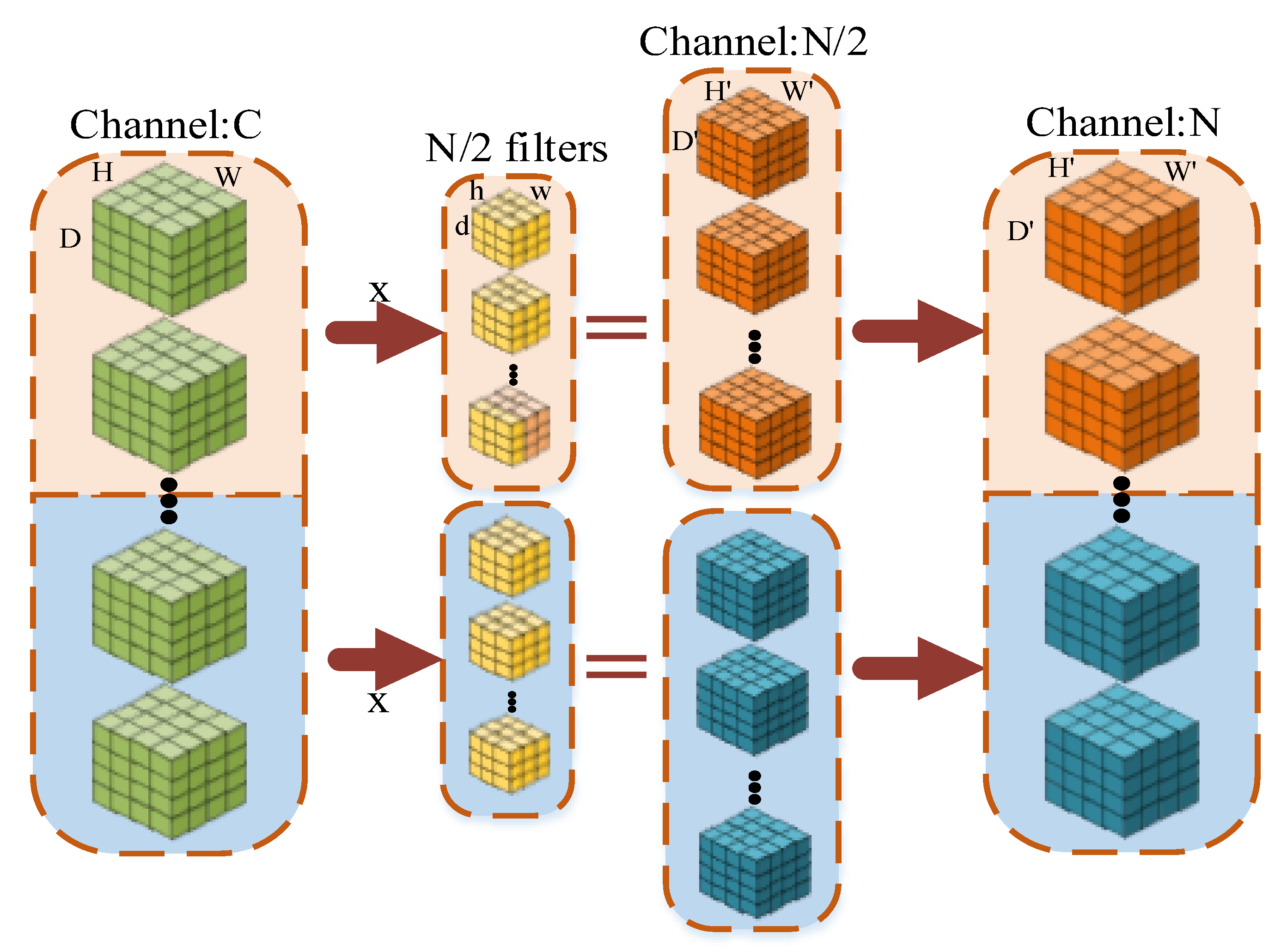
3.1. Branch-Fusion Net
3.2. Channel-Spatial Attention Module
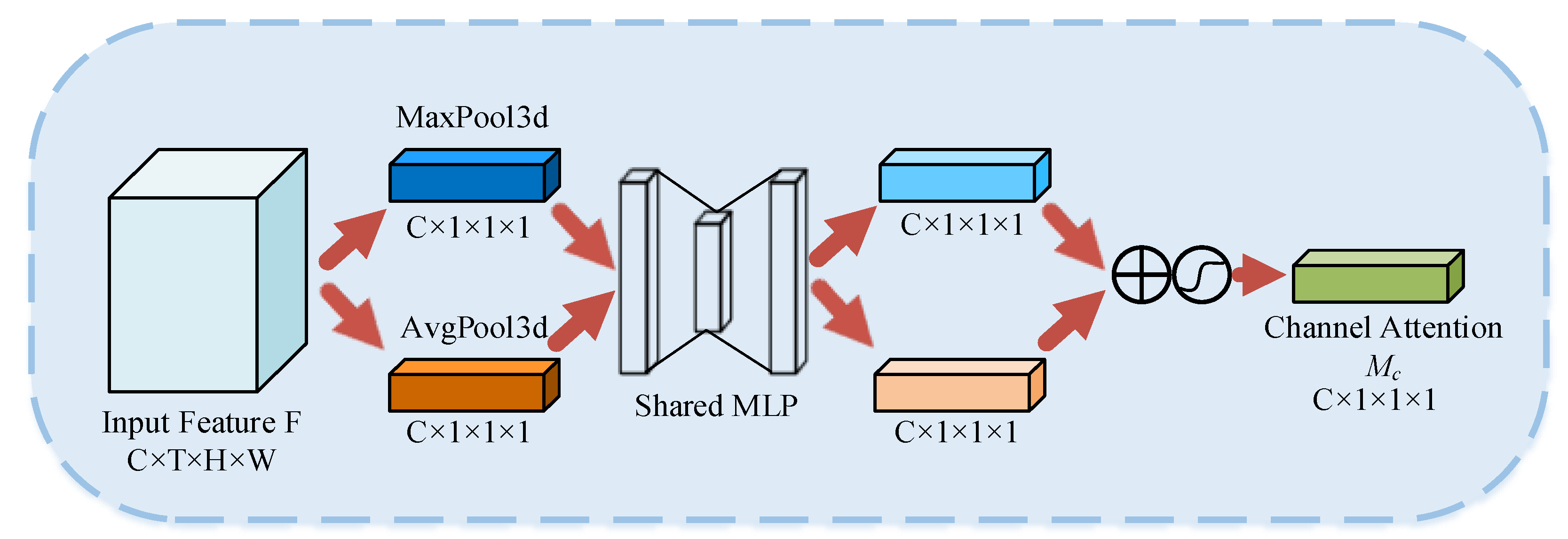
3.2.1. Channel Attention Module
 denotes the sigmoid activation function. Firstly, the spatiotemporal information of the input features was aggregated using three-dimensional average pooling and three-dimensional maximum pooling to generate two different spatiotemporal context descriptors. Then, the descriptors were fed into a multilayer perceptron with shared weights to obtain two feature maps. Finally, the two feature maps were summed element-by-element and activated by the sigmoid function to obtain the final channel attention weights. The CAM is computed as:
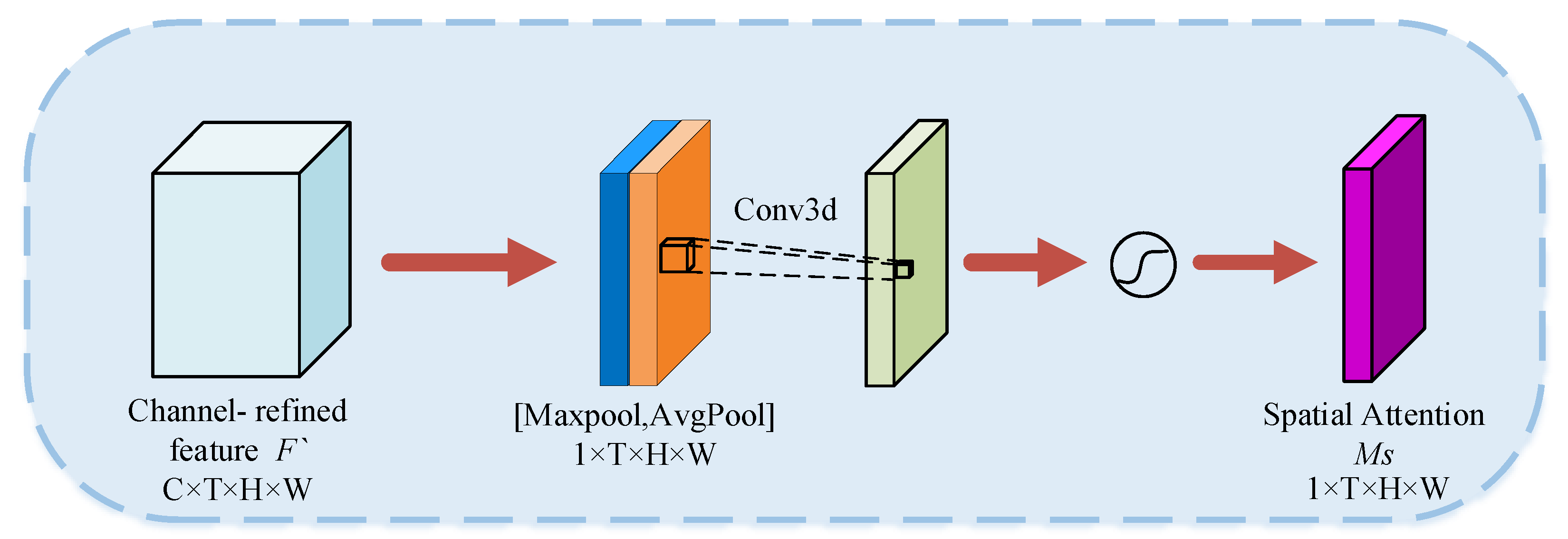
3.2.2. Spatial Attention Module
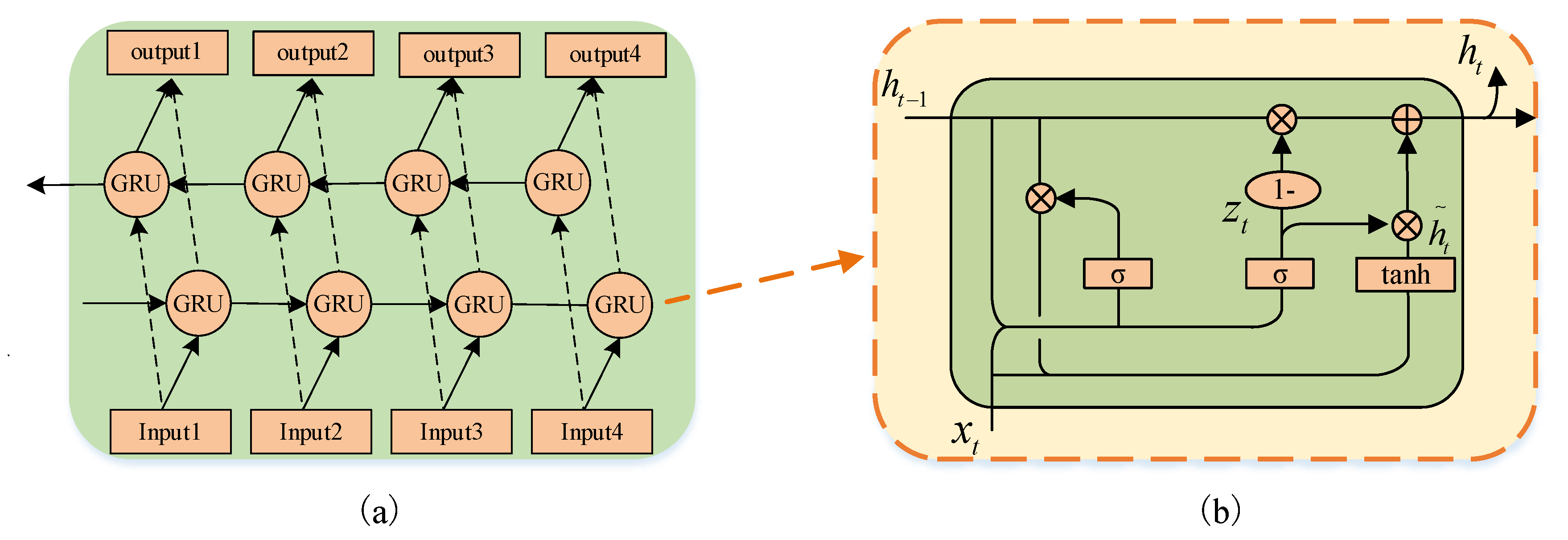
3.3. Bi-GRU
4. Experiment
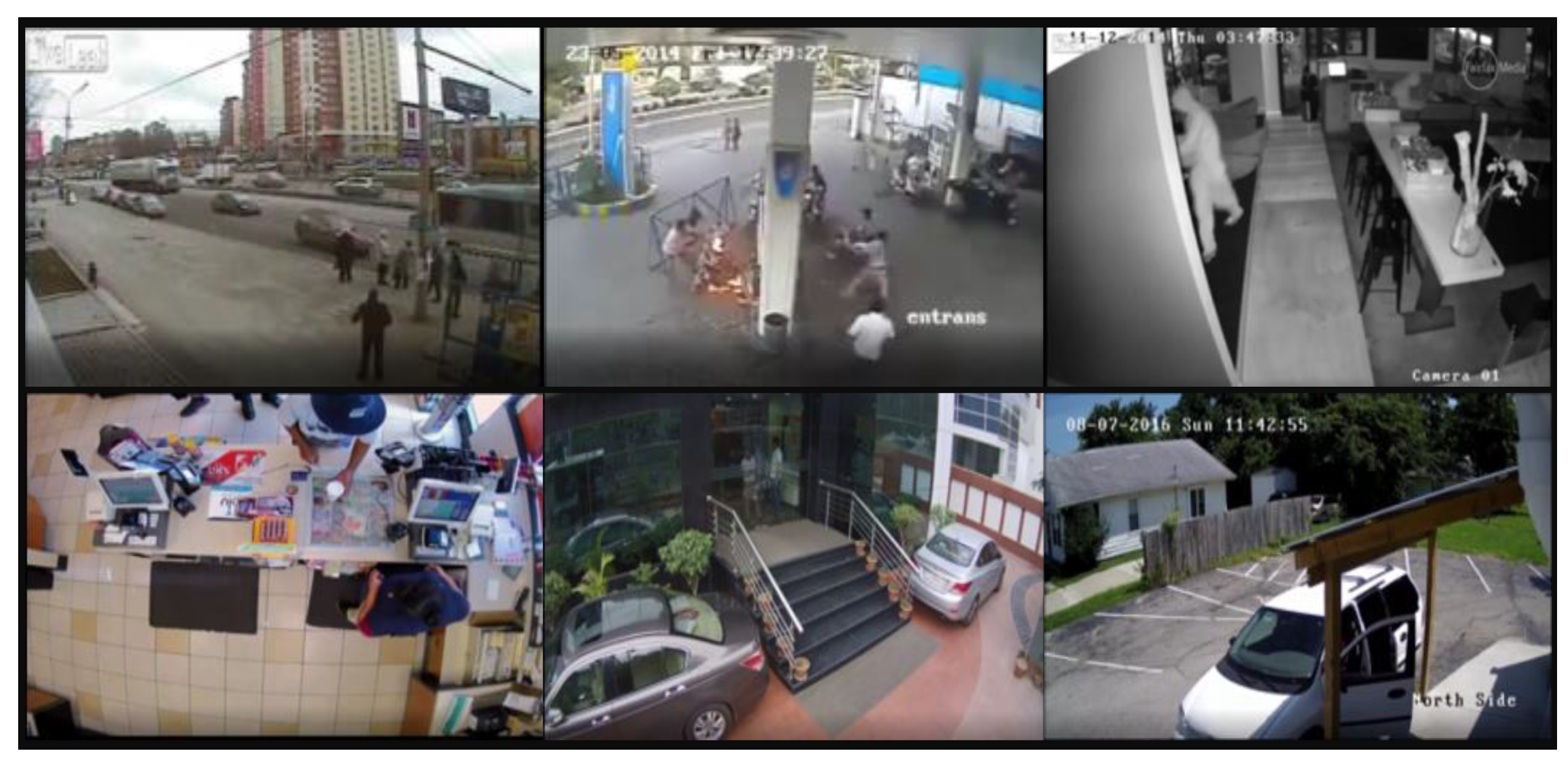
4.1. Dataset
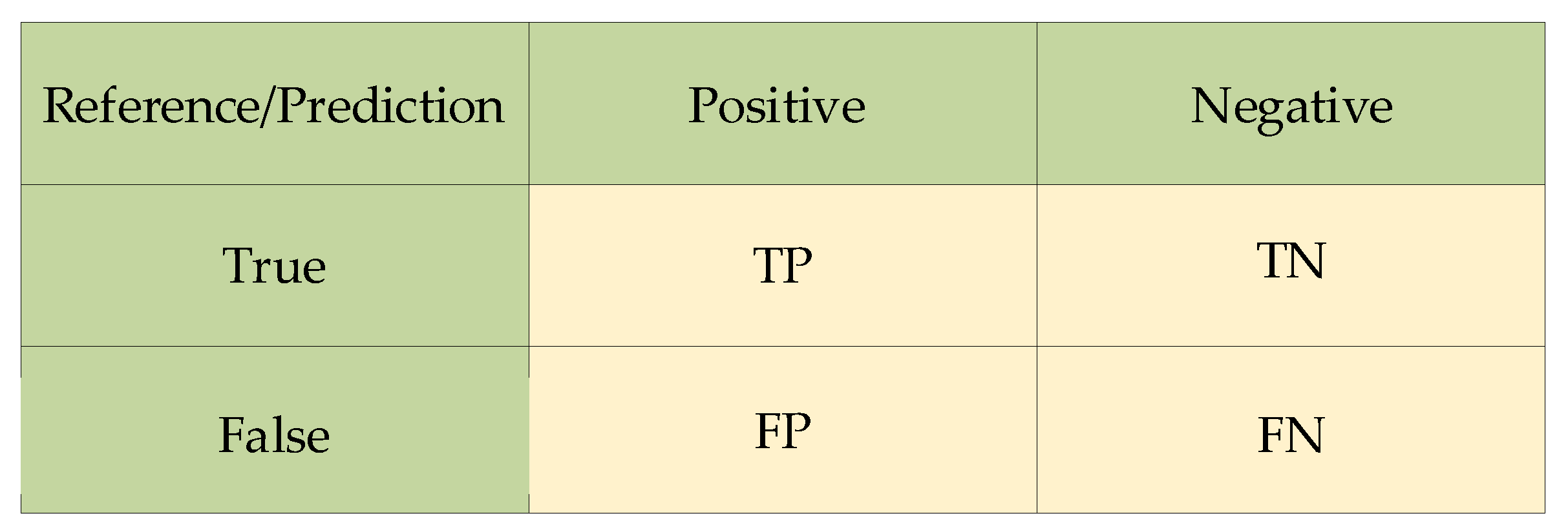
4.2. Evaluation Index
4.3. Hyperparameter Setting
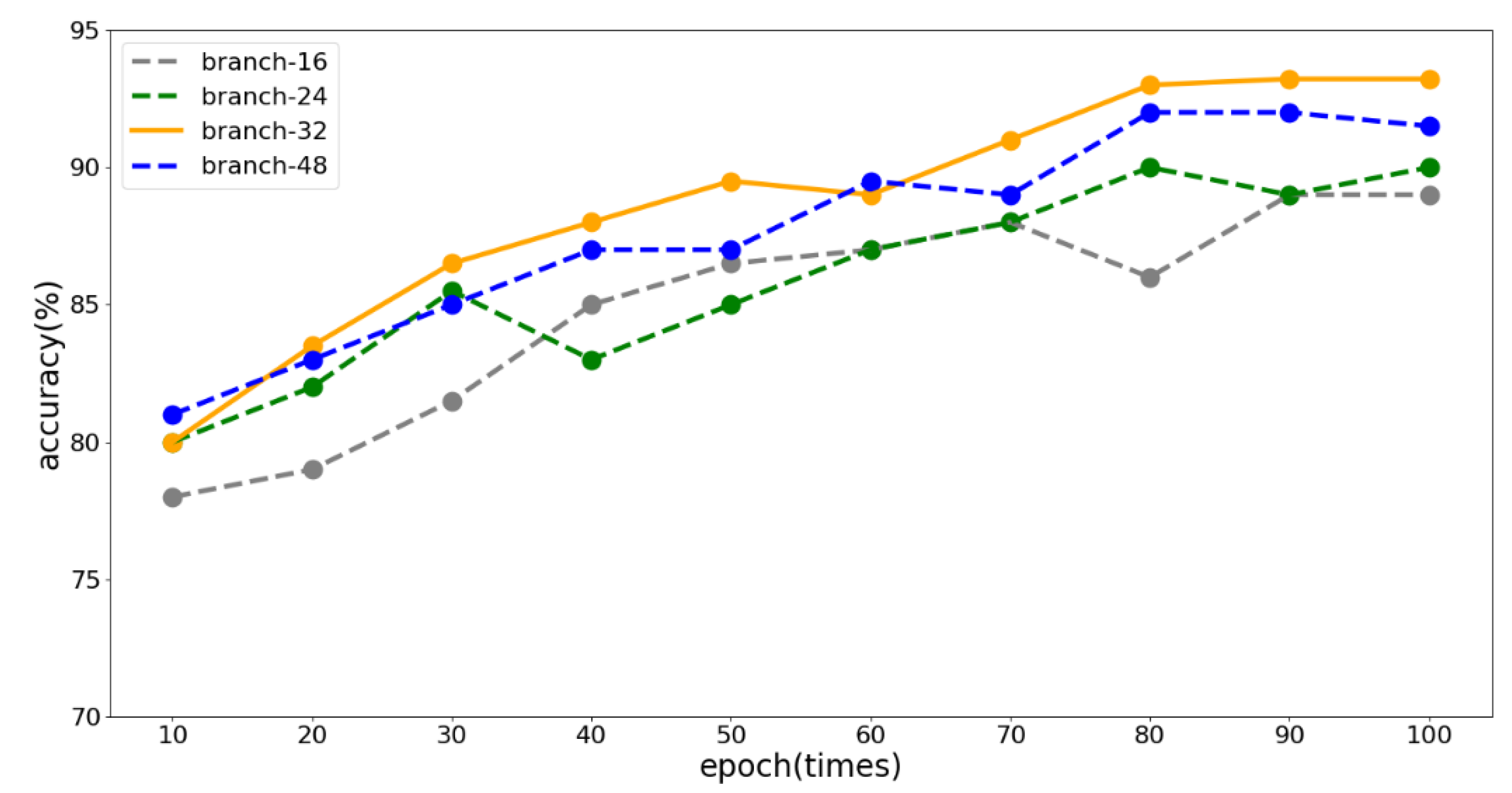
4.3.1. Number of Branches
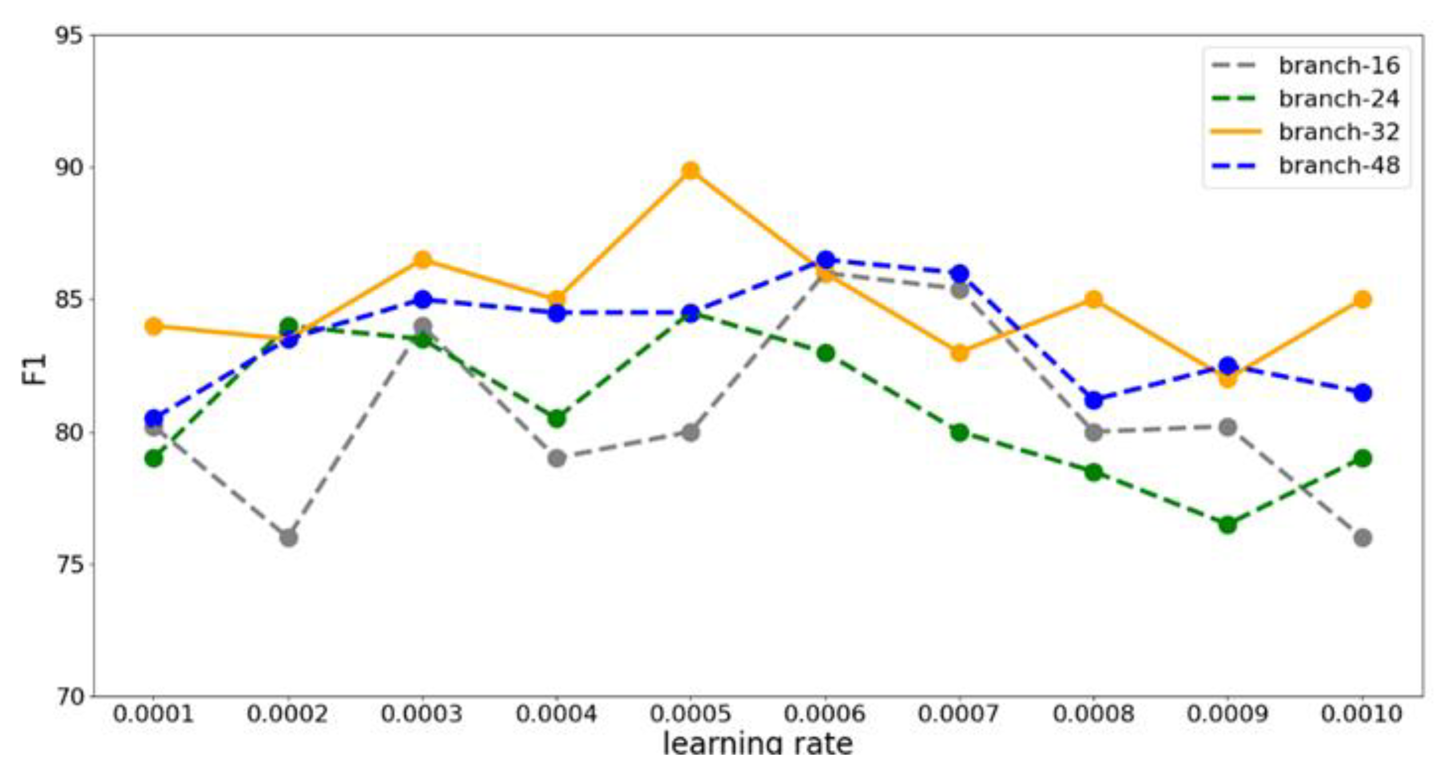
4.3.2. Learning Rate Setting
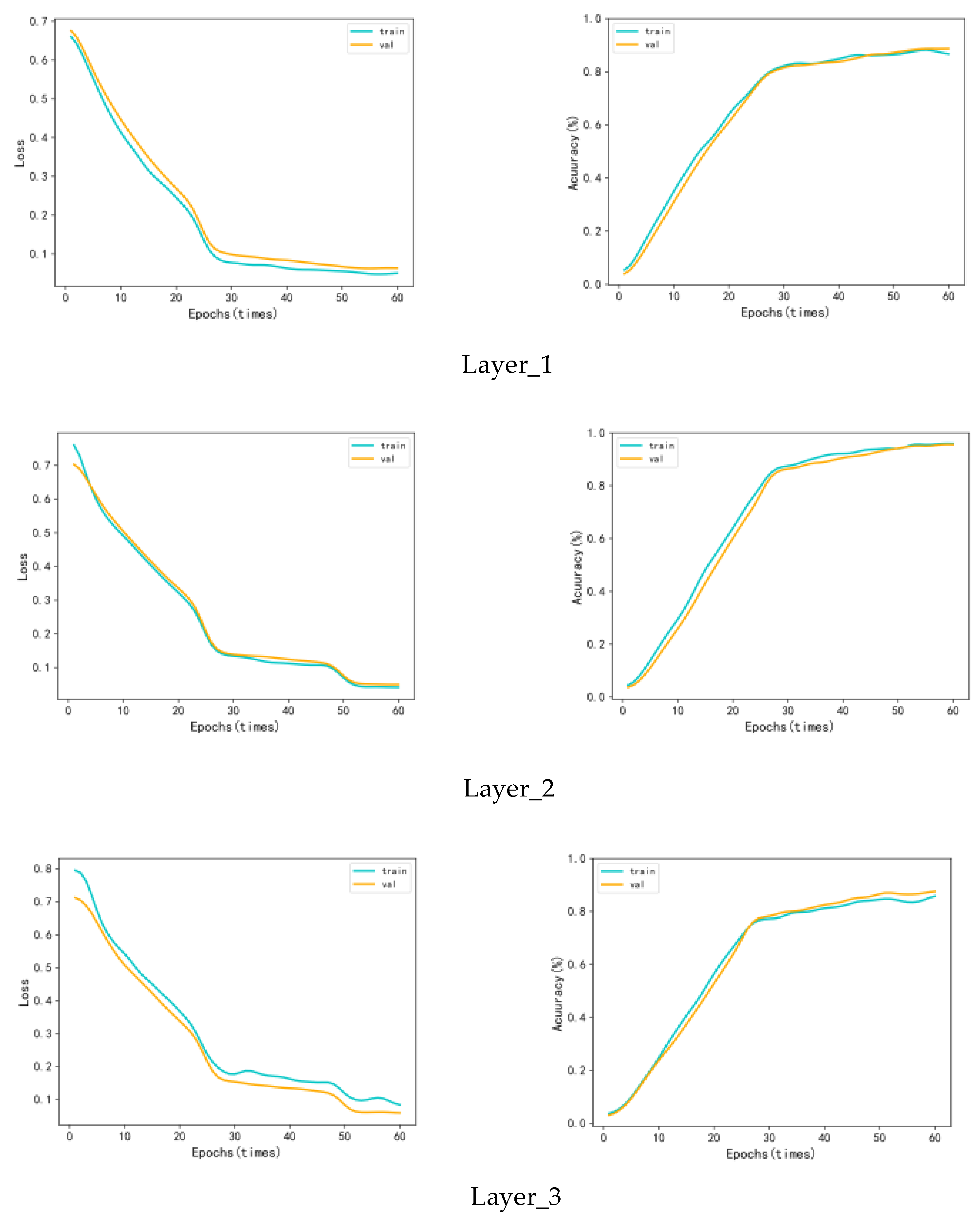
4.3.3. Number of Layers of Bi-GRU
4.4. Structure Setting of CSAM
4.5. Comparison Experiments with Branch-Fusion Net
4.6. Ablation Experiment of CSAM
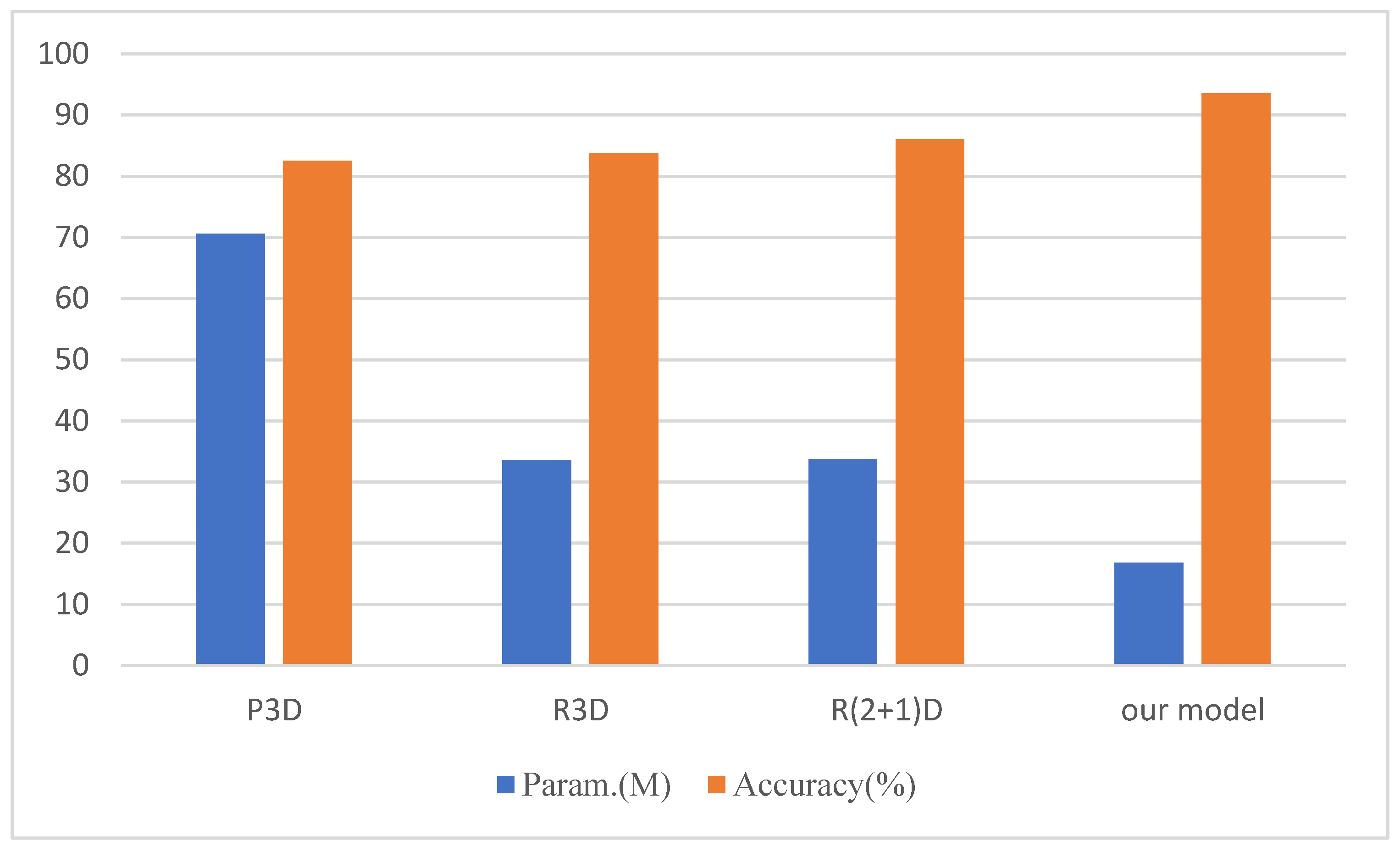
4.7. Comparison Experiment with Our Model
5. Conclusions
Author Contributions
Funding
Institutional Review Board Statement
Informed Consent Statement
Data Availability Statement
Conflicts of Interest
References
- Nayak, R.; Pati, U.C.; Das, S.K. A comprehensive review on deep learning-based methods for video anomaly detection. ScienceDirect 2020, 106, 104078. [Google Scholar] [CrossRef]
- Roshtkhari, M.J.; Levine, M.D. An on-line, real-time learning method for detecting anomalies in videos using spatio-temporal compositions. Comput. Vis. Image Underst. 2013, 117, 1436–1452. [Google Scholar] [CrossRef]
- Li, Y.; Cai, Y.; Liu, J.; Lang, S.; Zhang, X. Spatio-Temporal Unity Networking for Video Anomaly Detection. IEEE Access 2019, 7, 172425–172432. [Google Scholar] [CrossRef]
- Li, W.; Mahadevan, V.; Vasconcelos, N. Anomaly detection and localization in crowded scenes. IEEE Trans. Pattern Anal. Mach. Intell. 2014, 36, 18–32. [Google Scholar] [PubMed] [Green Version]
- Xu, D.; Ricci, E.; Yan, Y.; Song, J.; Sebe, N. Learning deep representations of appearance and motion for anomalous event detection. Comput. Vis. Image Underst. 2017, 156, 117–127. [Google Scholar] [CrossRef]
- Patraucean, V.; Handa, A.; Cipolla, R. Spatio-temporal video autoencoder with differentiable parameter. Comput. Sci. 2015, 58, 2415–2422. [Google Scholar]
- Zhao, B.; Li, F.F.; Xing, E.P. Online detection of unusual events in videos via dynamic sparse coding. In Proceedings of the IEEE Conference on Computer Vision & Pattern Recognition, Colorado Springs, CO, USA, 20–25 June 2011. [Google Scholar]
- Wang, X.Z.; Che, Z.P.; Jiang, B. Robust Unsupervised Video Anomaly Detection by Multipath Frame Prediction. IEEE Trans. Neural Netw. Learn. Syst. 2021, 33, 2301–2312. [Google Scholar] [CrossRef]
- Liu, W.; Luo, W.; Lian, D.; Gao, S. Future Frame Prediction for Anomaly Detection—A New Baseline. arXiv 2017, arXiv:1712.09867. [Google Scholar]
- Ionescu, R.T.; Khan, F.S.; Georgescu, M.I. Object-centric Auto-encoders and Dummy Anomalies for Abnormal Event Detection in Video. In Proceedings of the 2019 IEEE/CVF Conference on Computer Vision and Pattern Recognition (CVPR), Long Beach, CA, USA, 15–20 June 2019. [Google Scholar]
- Kiran, B.; Dilip, T.; Ranjith, P. An overview of deep learning based methods for unsupervised and semi-supervised anomaly detection in videos. J. Imaging 2018, 4, 36. [Google Scholar] [CrossRef] [Green Version]
- Tran, D.; Bourdev, L.; Fergus, R.; Torresani, L.; Paluri, M. Learning Spatiotemporal Features with 3D Convolutional Networks. In Proceedings of the 2015 IEEE International Conference on Computer Vision (ICCV), Santiago, Chile, 7–13 December 2015. [Google Scholar]
- Liang, Z.; Zhu, G.; Shen, P. Learning Spatiotemporal Features Using 3DCNN and Convolutional LSTM for Gesture Recognition. In Proceedings of the 2017 IEEE International Conference on Computer Vision Workshops (ICCVW), Venice, Italy, 22–29 October 2017. [Google Scholar]
- Ouyang, X.; Xu, S.; Zhang, C.; Zhou, P.; Yang, Y.; Liu, G.; Li, X. A 3D-CNN and LSTM Based Multi-Task Learning Architecture for Action Recognition. IEEE Access 2017, 7, 40757–40770. [Google Scholar] [CrossRef]
- Xu, X.; Liu, L.Q.; Zhang, L. Abnormal visual event detection based on multi instance learning and autoregressive integrated moving average model in edge-based Smart City surveillance. Softw. Pract. Exp. 2020, 50, 476–488. [Google Scholar] [CrossRef]
- Jie, H.; Li, S.; Gang, S. Squeeze-and-Excitation Networks. IEEE Trans. Pattern Anal. Mach. Intell. 2019, 42, 2021–2023. [Google Scholar]
- Li, K.; Wang, Y.; Zhang, J. UniFormer: Unifying Convolution and Self-attention for Visual Recognition. arXiv 2022, arXiv:2201.09450. [Google Scholar]
- Hasan, M.; Choi, J.; Neumann, J. Learning Temporal Regularity in Video Sequences. In Proceedings of the 2016 IEEE Conference on Computer Vision and Pattern Recognition (CVPR), Las Vegas, NV, USA, 27–30 June 2016. [Google Scholar]
- Gong, D.; Liu, L.; Le, V. Memorizing Normality to Detect Anomaly: Parameter-Augmented Deep Autoencoder for Unsupervised Anomaly Detection. In Proceedings of the 2019 IEEE/CVF International Conference on Computer Vision (ICCV), Seoul, Republic of Korea, 27 October–2 November 2019. [Google Scholar]
- Park, H.; Noh, J.; Ham, B. Learning Parameter-guided Normality for Anomaly Detection. arXiv 2020, arXiv:2003.13328. [Google Scholar]
- Medel, J.R.; Savakis, A. Anomaly Detection in Video Using Predictive Convolutional Long Short-Term Parameter Networks. arXiv 2016, arXiv:1612.00390. [Google Scholar]
- Lu, Y.; Reddy, M.; Nabavi, S.S. Future Frame Prediction Using Convolutional VRNN for Anomaly Detection. In Proceedings of the 2019 16th IEEE International Conference on Advanced Video and Signal Based Surveillance (AVSS), Taipei, Taiwan, 18–21 September 2019. [Google Scholar]
- Mathieu, M.; Couprie, C.; Lecun, Y. Deep multi-scale video prediction beyond mean square error. arXiv 2015, arXiv:1511.05440. [Google Scholar]
- Ye, M.; Peng, X.; Gan, W. AnoPCN: Video Anomaly Detection via Deep Predictive Coding Network. In Proceedings of the 27th ACM International Conference on Multimedia, Nice, France, 21–25 October 2019. [Google Scholar]
- Sabokrou, M.; Khalooei, M.; Fathy, M.; Adeli, E. Adversarially Learned One-Class Classifier for Novelty Detection. In Proceedings of the 2018 IEEE/CVF Conference on Computer Vision and Pattern Recognition, Salt Lake City, UT, USA, 18–23 June 2018. [Google Scholar]
- Wu, P.; Liu, J.; Shen, F. A Deep One-Class Neural Network for Anomalous Event Detection in Complex Scenes. IEEE Trans. Neural Netw. Learn. Syst. 2020, 31, 2609–2622. [Google Scholar] [CrossRef] [PubMed]
- Xu, K.; Sun, T.; Jiang, X. Video Anomaly Detection and Localization Based on an Adaptive Intra-frame Classification Network. IEEE Trans. Multimed. 2020, 22, 394–406. [Google Scholar] [CrossRef]
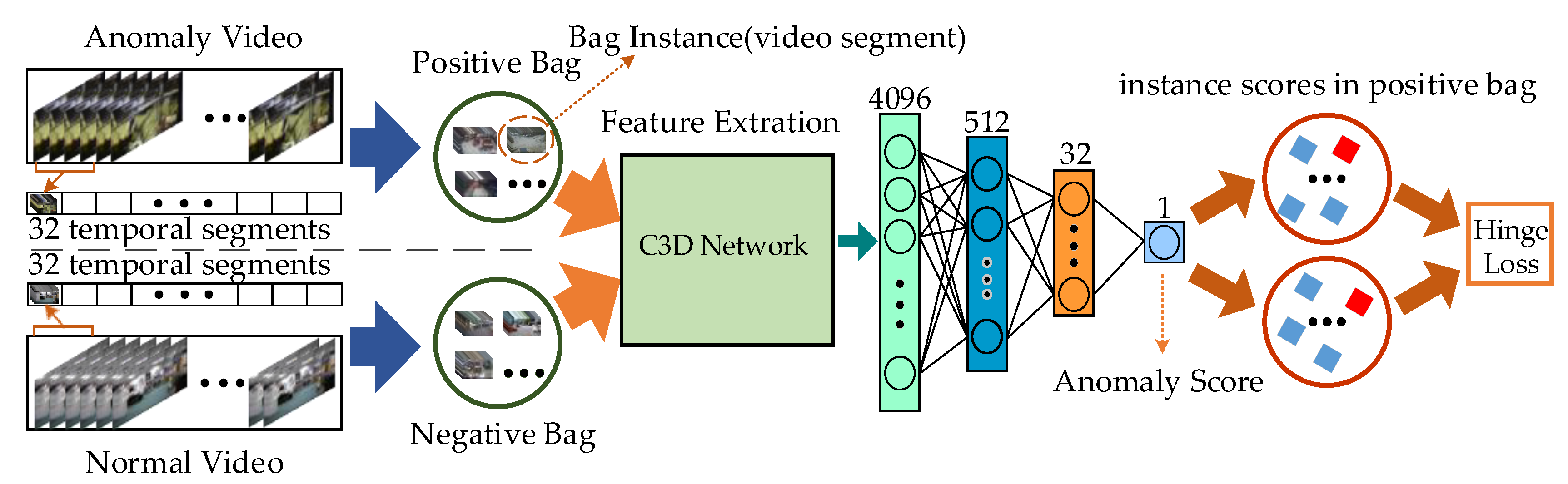
- Sultani, W.; Chen, C.; Shah, M. Real-World Anomaly Detection in Surveillance Videos. In Proceedings of the 2018 IEEE/CVF Conference on Computer Vision and Pattern Recognition, Salt Lake City, UT, USA, 18–23 June 2018. [Google Scholar]
- Kamoona, A.M.; Gosta, A.K.; Bab-Hadiashar, A. Multiple Instance-Based Video Anomaly Detection using Deep Temporal Encoding-Decoding. arXiv 2020, arXiv:2007.01548. [Google Scholar] [CrossRef]
- Zhu, Y.; Newsam, S. Motion-Aware Feature for Improved Video Anomaly Detection. arXiv 2019, arXiv:1907.10211. [Google Scholar]
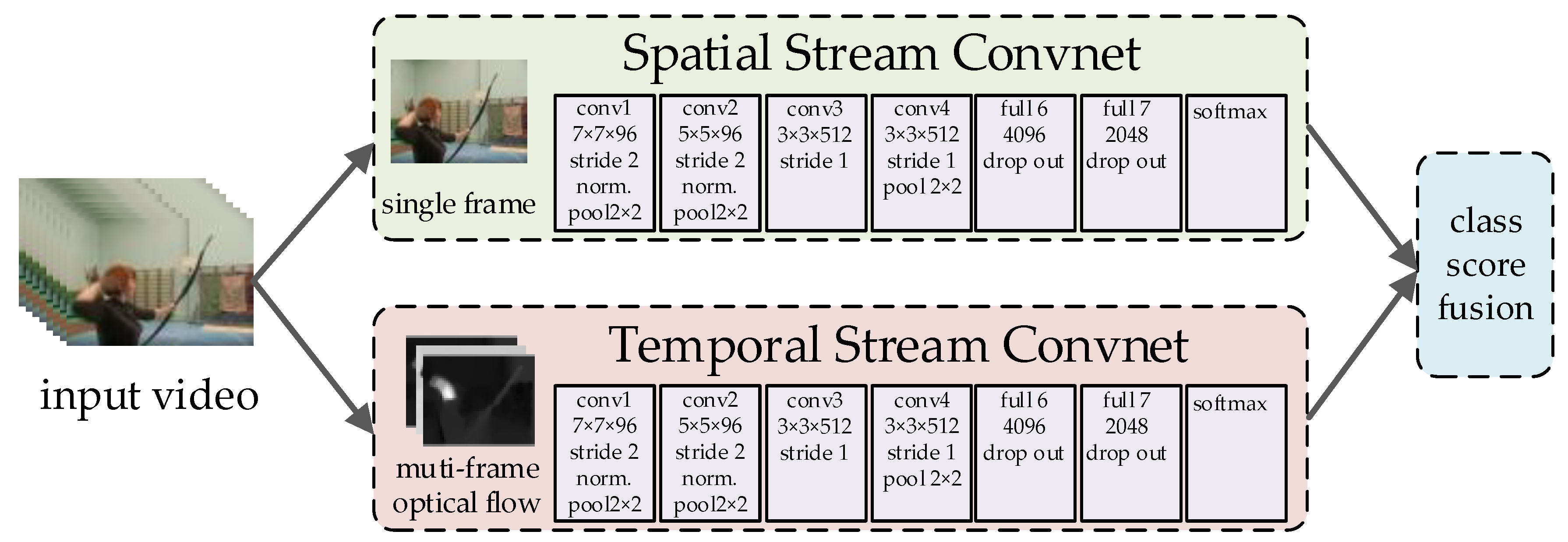
- Simonyan, K.; Zisserman, A. Two-Stream Convolutional Networks for Action Recognition in Videos. In Proceedings of the 27th International Conference on Neural Information Processing Systems, Montreal, QC, Canada, 8 December 2014. [Google Scholar]
- Carreira, J.; Zisserman, A. Quo Vadis, Action Recognition? A New Model and the Kinetics Dataset. In Proceedings of the 2017 IEEE Conference on Computer Vision and Pattern Recognition (CVPR), Honolulu, HI, USA, 21–26 July 2017. [Google Scholar]
- Wang, L.; Xiong, Y.; Wang, Z.; Qiao, Y.; Lin, D.; Tang, X.; Van Gool, L. Temporal Segment Networks: Towards Good Practices for Deep Action Recognition. arXiv 2016, arXiv:1608.00859. [Google Scholar]
- Lin, J.; Gan, C.; Han, S. TSM: Temporal Shift Module for Efficient Video Understanding. In Proceedings of the 2019 IEEE/CVF International Conference on Computer Vision (ICCV), Seoul, Republic of Korea, 27 October–2 November 2019. [Google Scholar]
- Li, Y.; Ji, B.; Shi, X.; Zhang, J.; Kang, B.; Wang, L. TEA: Temporal Excitation and Aggregation for Action Recognition. In Proceedings of the 2020 IEEE/CVF Conference on Computer Vision and Pattern Recognition (CVPR), Seattle, WA, USA, 13–19 June 2020. [Google Scholar]
- Wang, L.; Tong, Z.; Ji, B.; Wu, G. TDN: Temporal Difference Networks for Efficient Action Recognition. In Proceedings of the 2021 IEEE/CVF Conference on Computer Vision and Pattern Recognition (CVPR), Nashville, TN, USA, 20–25 June 2021. [Google Scholar]
- Feichtenhofer, C.; Fan, H.; Malik, J.; He, K. SlowFast Networks for Video Recognition. In Proceedings of the 2019 IEEE/CVF International Conference on Computer Vision (ICCV), Seoul, Republic of Korea, 27 October–2 November 2019. [Google Scholar]
- Hara, K.; Kataoka, H.; Satoh, Y. Learning Spatio-Temporal Features with 3D Residual Networks for Action Recognition. In Proceedings of the 2017 IEEE International Conference on Computer Vision Workshops (ICCVW), Venice, Italy, 22–29 October 2017. [Google Scholar]
- Tran, D.; Wang, H.; Torresani, L.; Ray, J.; LeCun, Y.; Paluri, M. A Closer Look at Spatiotemporal Convolutions for Action Recognition. In Proceedings of the 2018 IEEE/CVF Conference on Computer Vision and Pattern Recognition, Salt Lake City, UT, USA, 18–23 June 2018. [Google Scholar]
- Xie, S.; Sun, C.; Huang, J.; Tu, Z.; Murphy, K. Rethinking Spatiotemporal Feature Learning: Speed-Accuracy Trade-offs in Video Classification. arXiv 2017, arXiv:1712.04851. [Google Scholar]
- Feichtenhofer, C. X3D: Expanding Architectures for Efficient Video Recognition. In Proceedings of the 2020 IEEE/CVF Conference on Computer Vision and Pattern Recognition (CVPR), Seattle, WA, USA, 13–19 June 2020. [Google Scholar]
- Wang, X.; Girshick, R.; Gupta, A.; He, K. Non-Local Neural Networks. In Proceedings of the IEEE Conference on Computer Vision and Pattern Recognition (CVPR), Salt Lake City, UT, USA, 18–23 June 2018. [Google Scholar]
- Qiu, Z.; Yao, T.; Mei, T. Learning Spatio-Temporal Representation with Pseudo-3D Residual Networks. In Proceedings of the 2017 IEEE International Conference on Computer Vision (ICCV), Venice, Italy, 22–29 October 2017. [Google Scholar]


| Category | Judgment Basis | Advantages | Disadvantages |
|---|---|---|---|
| Reconstruction-based method | Small reconstruction errors for normal video frames and large reconstruction errors for abnormal video frames. | High accuracy in detecting location-related anomalies. | There are reconstruction errors for anomalous video frames. |
| Prediction-based method | Small prediction errors for normal video frames and large prediction errors for abnormal video frames. | High accuracy in detecting motion-related anomalies. | It ignores the fact that normal video frames can be unpredictable. |
| Classification-based method | The samples that do not follow the normal sample distribution are considered abnormal. | The distribution of normal samples can be well-learned. | If the normal sample distribution is complex, the classification model may fail. |
| Regression-based method | The samples with anomaly scores above the threshold are considered abnormal. | The model is simple and suitable for large-scale video anomaly detection. | The threshold for video anomalies is not easy to determine. |
| Layer Name | Size | Stride |
|---|---|---|
| Conv1a | 3 × 3 × 3 | 1 × 1 × 1 |
| pool1 | 1 × 2 × 2 | 1 × 2 × 2 |
| Conv2a | 3 × 3 × 3 | 1 × 1 × 1 |
| Pool2 | 2 × 2 × 2 | 2 × 2 × 2 |
| Conv3a | 3 × 3 × 3 | 1 × 1 × 1 |
| Conv3b | 3 × 3 × 3 | 1 × 1 × 1 |
| pool3 | 2 × 2 × 2 | 2 × 2 × 2 |
| Conv4a | 3 × 3 × 3 | 1 × 1 × 1 |
| Conv4b | 3 × 3 × 3 | 1 × 1 × 1 |
| pool4 | 2 × 2 × 2 | 2 × 2 × 2 |
| Conv5a | 3 × 3 × 3 | 1 × 1 × 1 |
| Conv5b | 3 × 3 × 3 | 1 × 1 × 1 |
| pool5 | 2 × 2 × 2 | 2 × 2 × 2 |
| Stage | Output Size | The Size of the Stage |
|---|---|---|
| Conv1 | ||
| Conv2 | ||
| Conv3 | ||
| Conv4 | ||
| Conv5 | ||
| AvgPooling and Flattening | ||
| FC0 | ||
| Bi-GRU | Hidden_size = 128 Num_layer = 2 | |
| FC1 | ||
| FC2 |
| Anomaly | No. of Videos |
|---|---|
| Arson | 100 |
| Burglary | 100 |
| Explosion | 100 |
| Road accident | 150 |
| Stealing | 120 |
| Normal events | 320 |
| Description | Accuracy (%) |
|---|---|
| Model (Branch-Fusion Net) | 86.29 |
| model + CAM | 89.56 |
| model + SAM | 90.08 |
| model + CAM and SAM in parallel | 93.57 |
| model + SAM + CAM | 92.83 |
| model + CAM + SAM | 93.43 |
| Architecture | UCF-101 | HMDB51 |
|---|---|---|
| Two-Stream [31] | 87.84 | 58.86 |
| TSN [33] | 93.90 | 70.88 |
| TSM [34] | 95.47 | 73.95 |
| TEA [35] | 96.63 | 73.12 |
| TDN [36] | 95.39 | 76.26 |
| SlowFast [37] | 96.20 | 78.04 |
| C3D [12] | 85.08 | 56.00 |
| R3D [38] | 85.22 | 53.80 |
| R(2 + 1)D [39] | 95.55 | 73.85 |
| S3D [40] | 96.62 | 75.33 |
| X3D [41] | 96.71 | 81.67 |
| Two-Stream I3D [32] | 97.29 | 80.71 |
| NL I3D [42] | 96.87 | 80.16 |
| Branch-Fusion Net | 97.32 | 82.14 |
| Description | TOP-1 | TOP-5 |
|---|---|---|
| TSN [33] | 68.93 | 87.84 |
| TSM [34] | 74.39 | 90.89 |
| TEA [35] | 76.20 | 92.27 |
| TDN [36] | 76.85 | 93.16 |
| S3D [40] | 74.69 | 93.24 |
| X3D [41] | 79.06 | 93.76 |
| R(2 + 1)D [39] | 74.28 | 91.49 |
| SlowFast [37] | 77.11 | 92.37 |
| Two-Stream I3D [32] | 72.02 | 89.89 |
| NL I3D [42] | 76.38 | 92.55 |
| Branch-Fusion Net | 80.03 | 93.81 |
| Architecture | Params/M | Accuracy (%) |
|---|---|---|
| C3D | 58.378 | 72.93 |
| C3D + CSAM | 58.454 | 77.71 |
| R3D | 33.642 | 80.29 |
| R3D + CSAM | 33.731 | 83.90 |
| R(2 + 1)D | 33.641 | 83.08 |
| R(2 + 1)D + CSAM | 33.730 | 88.44 |
| Branch-Fusion Net | 14.856 | 89.63 |
| Branch-Fusion Net + CSAM | 16.190 | 93.55 |
Disclaimer/Publisher’s Note: The statements, opinions and data contained in all publications are solely those of the individual author(s) and contributor(s) and not of MDPI and/or the editor(s). MDPI and/or the editor(s) disclaim responsibility for any injury to people or property resulting from any ideas, methods, instructions or products referred to in the content. |
© 2023 by the authors. Licensee MDPI, Basel, Switzerland. This article is an open access article distributed under the terms and conditions of the Creative Commons Attribution (CC BY) license (https://creativecommons.org/licenses/by/4.0/).
Share and Cite
Zhang, P.; Lu, Y. Research on Anomaly Detection of Surveillance Video Based on Branch-Fusion Net and CSAM. Sensors 2023, 23, 1385. https://doi.org/10.3390/s23031385
Zhang P, Lu Y. Research on Anomaly Detection of Surveillance Video Based on Branch-Fusion Net and CSAM. Sensors. 2023; 23(3):1385. https://doi.org/10.3390/s23031385
Chicago/Turabian StyleZhang, Pengjv, and Yuanyao Lu. 2023. "Research on Anomaly Detection of Surveillance Video Based on Branch-Fusion Net and CSAM" Sensors 23, no. 3: 1385. https://doi.org/10.3390/s23031385