
Time-Domain Numerical Simulation and Experimental Study on Pulsed Eddy Current Inspection of Tubing and Casing
Abstract
:1. Introduction
2. Basic Principle of Pulse Eddy Current Detecting Tubing and Casing
3. Results
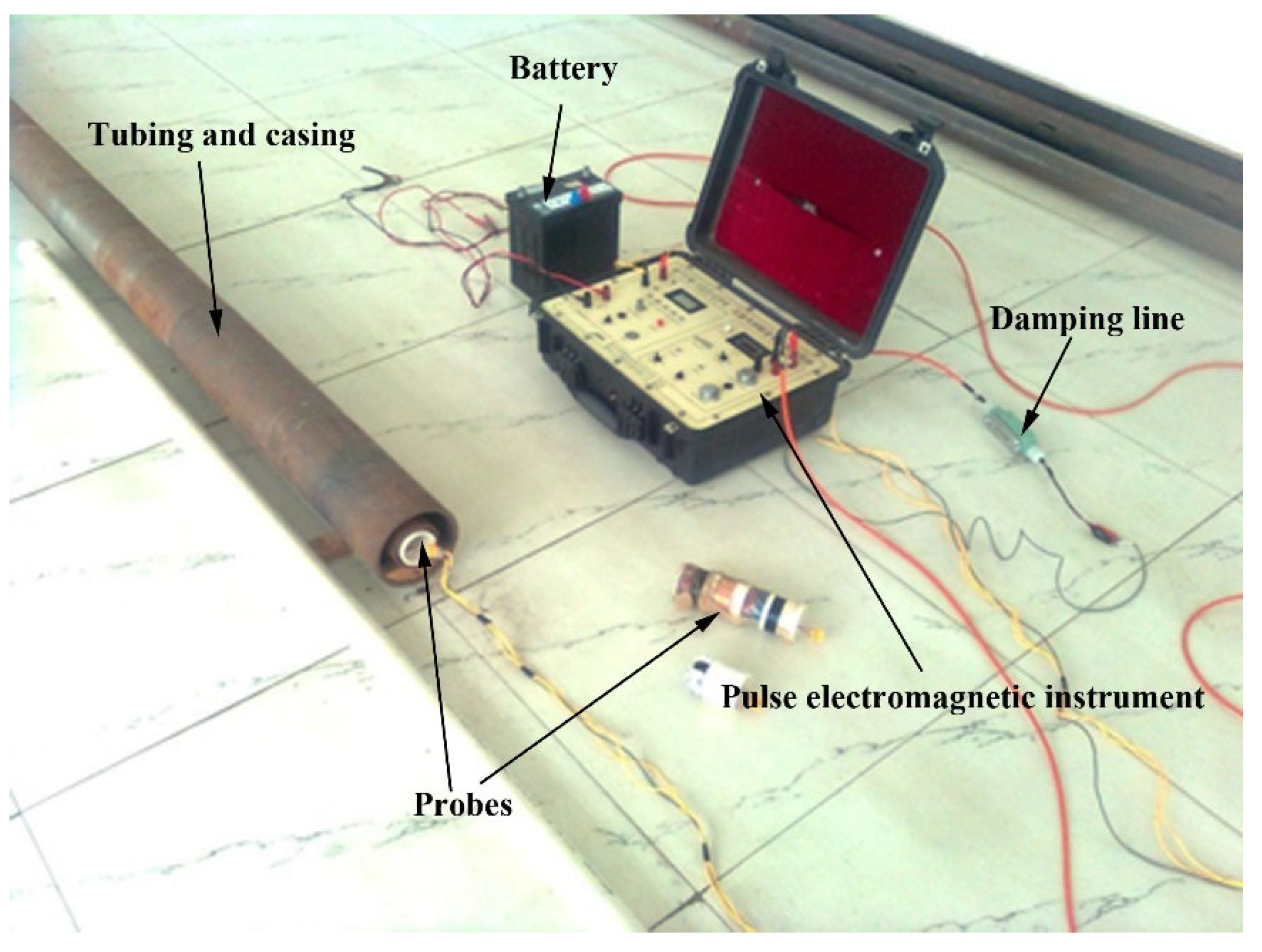
3.1. Experiment Apparatus
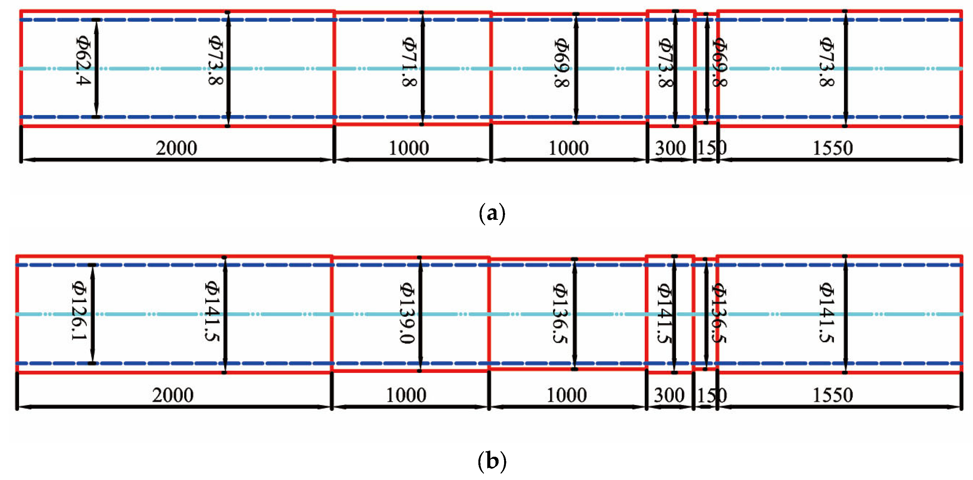
3.2. Test Specimens
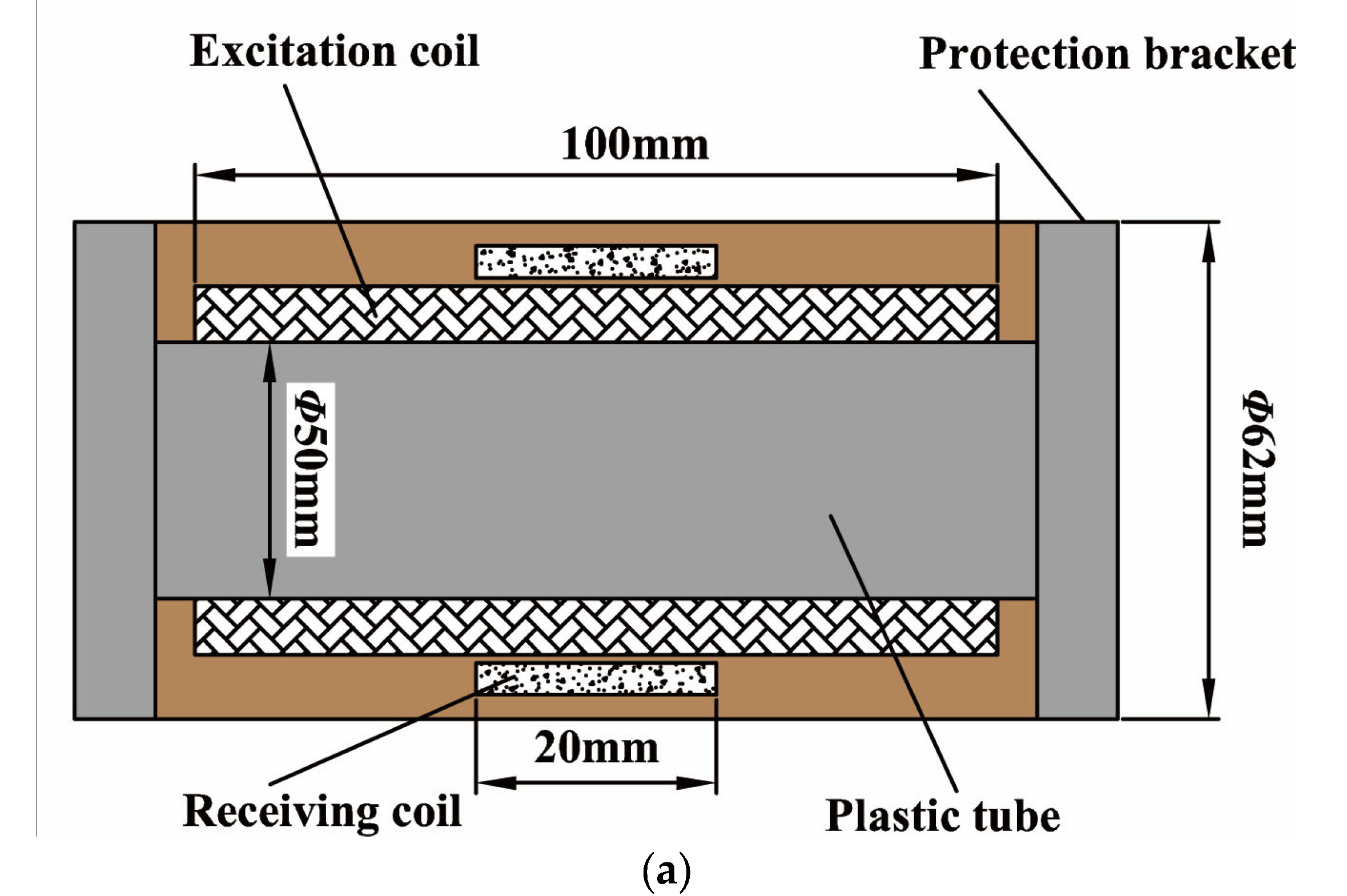
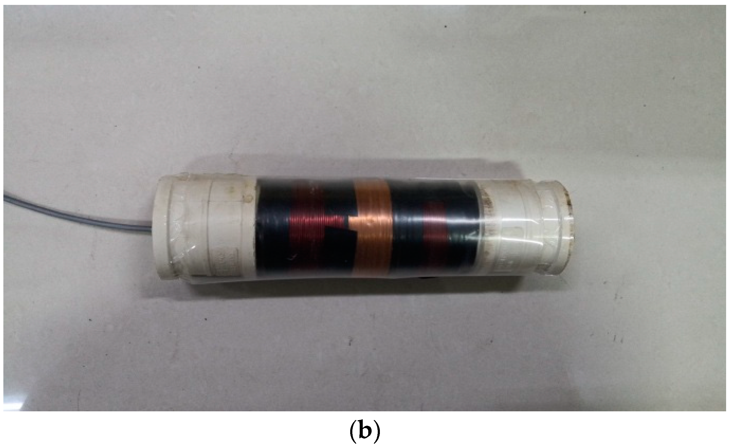
3.3. Probe Design
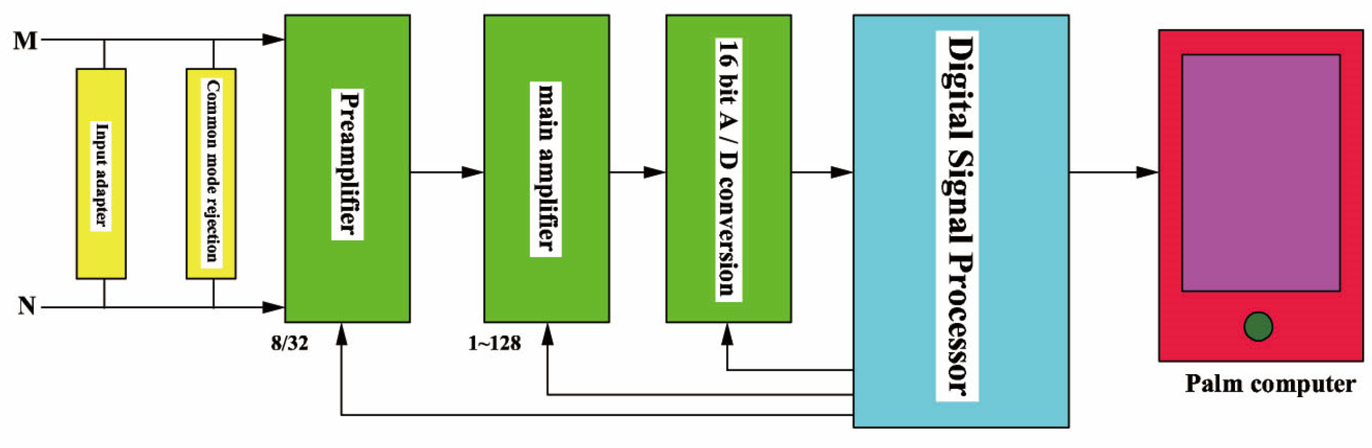
3.4. Processing Method of Inspection Data
3.5. Evaluation Criteria for Inspection Sensitivity
4. Finite Element Simulation Analysis
4.1. Simulation Model Establishment
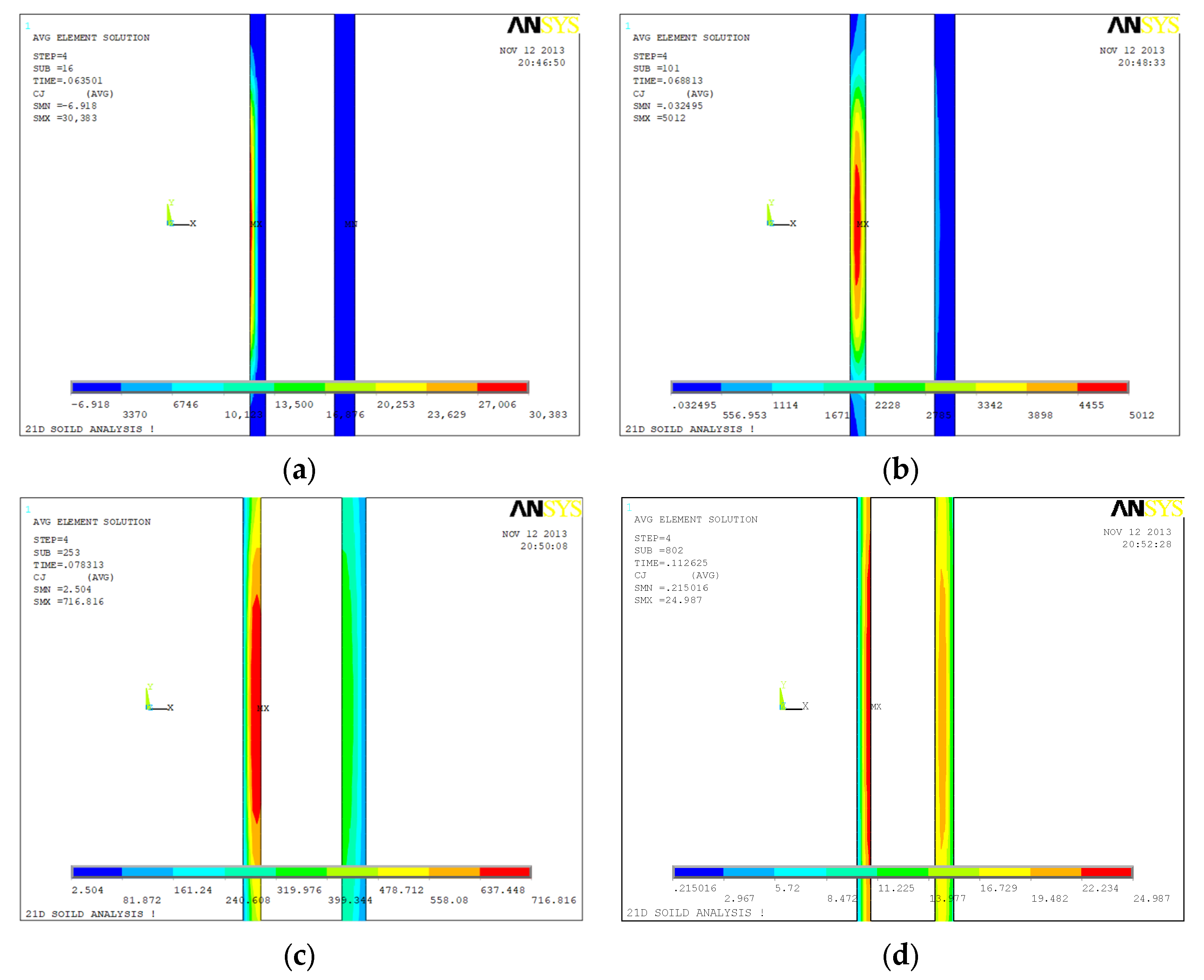
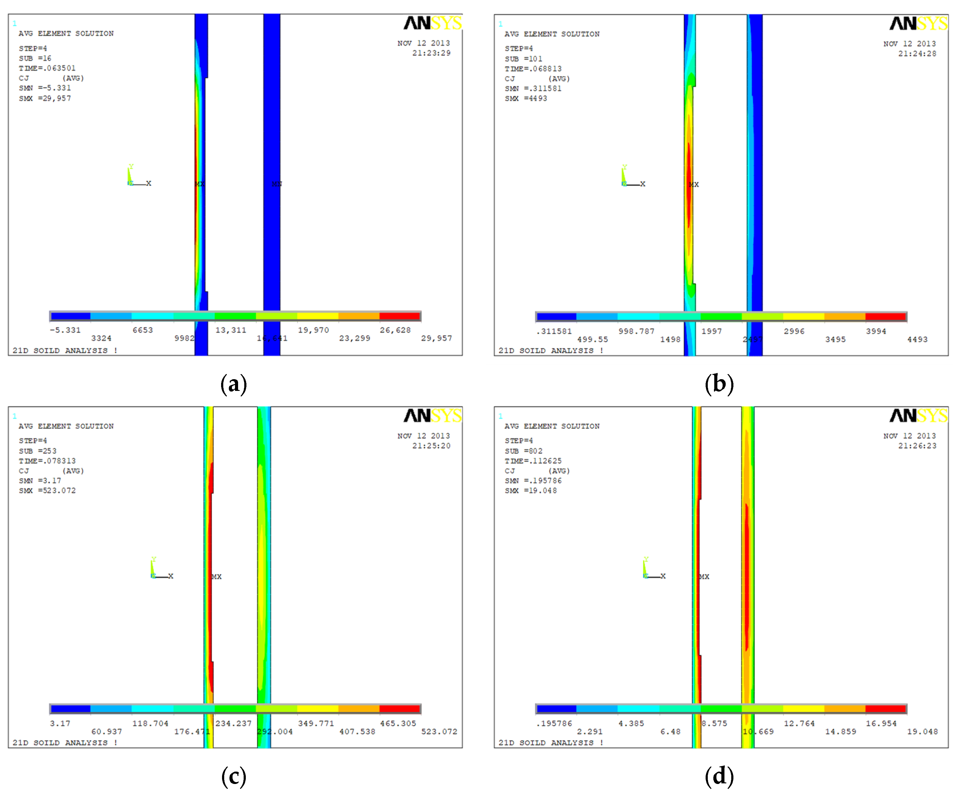
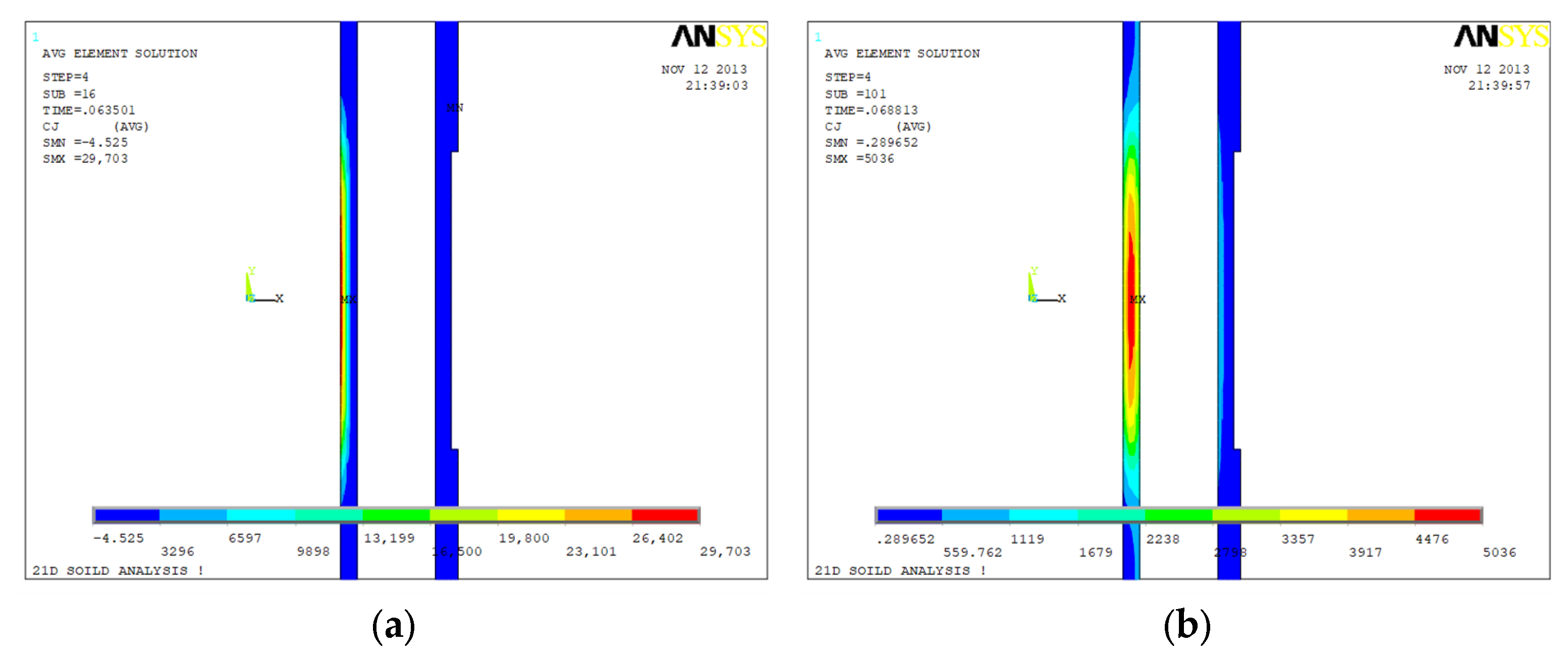
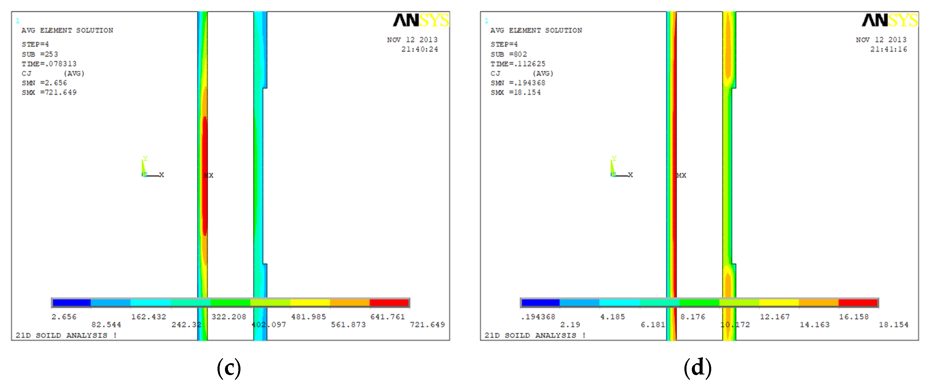
4.2. Time Domain Dynamic Analysis of Eddy Current Field Distribution
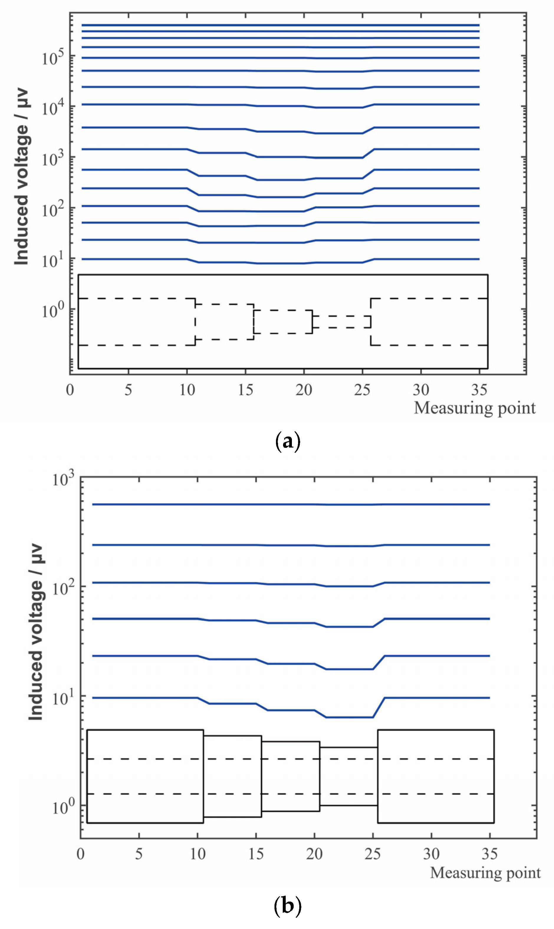
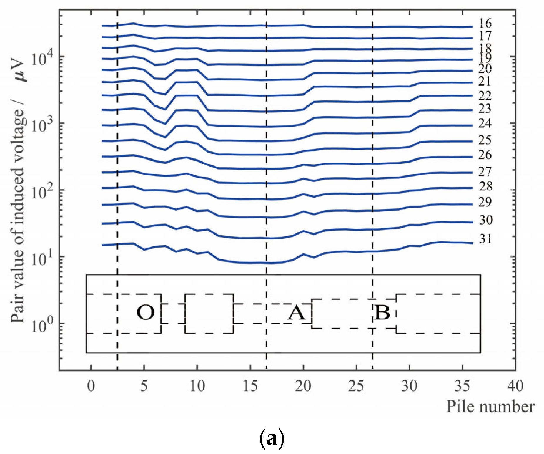
4.3. Time Slice Analysis of the Receiving Coil Induced Voltage

| Corrosion Depth | Tubing Corroding 1.25 mm | Tubing Corroding 2.5 mm | Tubing Corroding 3.75 mm | Casing Corroding 1.25 mm | Casing Corroding 2.5 mm | Casing Corroding 3.75 mm |
|---|---|---|---|---|---|---|
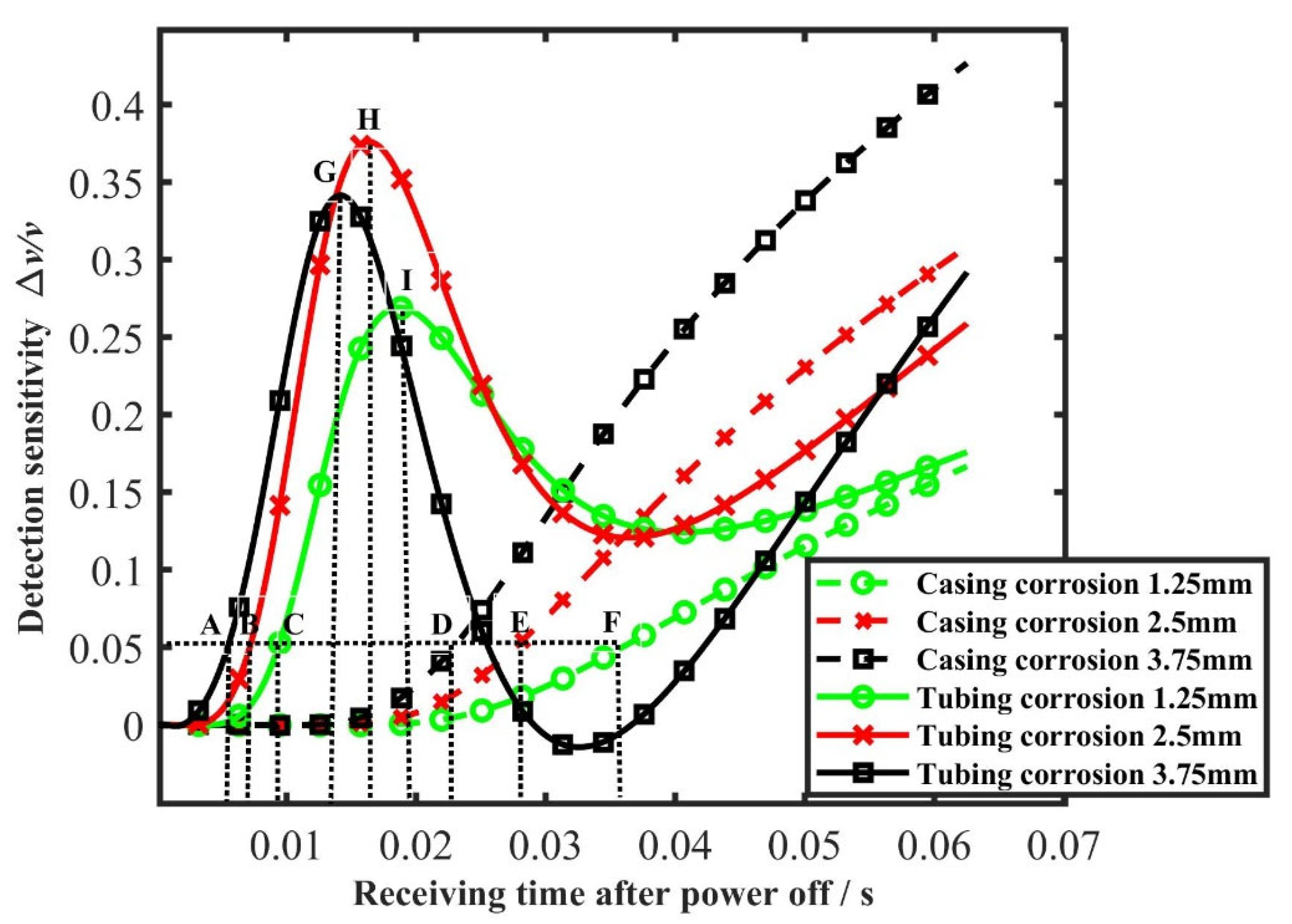
| Up to 5% moments (after power off) /s | 0.0094 (point C) | 0.0072 (point B) | 0.0054 (point A) | 0.0359 (point F) | 0.0275 (point E) | 0.0229 (point D) |
| Up to 5% moments (absolute value) /s | 0.0719 | 0.0697 | 0.0679 | 0.0984 | 0.0900 | 0.0854 |
| Peak time (after power off) /s | 0.0196 (point I) | 0.0164 (point H) | 0.0142 (point G) | 0.0625 (end) | 0.0625 (end) | 0.0625 (end) |
| Peak time (absolute value) /s | 0.0821 | 0.0789 | 0.0767 | 0.1250 | 0.1250 | 0.1250 |
5. Experiments and Analysis
5.1. Experiments
5.2. Analysis and Discussion
6. Conclusions and Future Work
Author Contributions
Funding
Institutional Review Board Statement
Informed Consent Statement
Data Availability Statement
Conflicts of Interest
References
- Heidersbach, R. Metallurgy and Corrosion Control in Oil and Gas Production; Wiley: Hoboken, NJ, USA, 2011; pp. 75–109. [Google Scholar]
- Li, Q.; Liu, B. Erosion-Corrosion of Gathering Pipeline Steel in Oil-Water-Sand Multiphase Flow. Metals 2023, 13, 80. [Google Scholar] [CrossRef]
- Zvirko, O.; Tsyrulnyk, O.; Lipiec, S.; Dzioba, I. Evaluation of Corrosion, Mechanical Properties and Hydrogen Embrittlement of Casing Pipe Steels with Different Microstructure. Materials 2021, 14, 7860. [Google Scholar] [CrossRef] [PubMed]
- Wang, T.; Yang, S.; Zhu, W.; Bian, W.; Lin, M.; Lei, Y.; Zhang, Y.; Zhang, J.; Zhao, W.; Chen, L.; et al. Law and countermeasures for the casing damage of oil production wells and water injection wells in Tarim Oilfield. Pet. Explor. Dev. 2011, 38, 352–361. [Google Scholar]
- Qian, J.; Tang, Z.H.; Guan, L.; Wang, W.C.; Du, S.F. Logging Application and Contrast Analysis of Casing Failure. J. Southwest Pet. Inst. 2004, 26, 73–76. [Google Scholar]
- Sun, Y.C.; Zheng, H.; Cui, Y.H. The Multilayer Case-pipes Electromagnetic Defect Detecting Logging. Well Logging Technol. 2003, 27, 246–250. [Google Scholar]
- Zhou, L.F. The application of electromagnetism inspection technique in Jiangsu oilfield. Well Test. 2003, 12, 48–49. [Google Scholar]
- Liu, H.L.; Wang, C.R.; Du, J.P.; Zhang, B.; Luo, X.M. Combined Logging Application of 40-arm Caliper Imaging and Electro-magnetic Defect Detection Technology in Tuha Oilfield. Well Logging Technol. 2012, 36, 416–420. [Google Scholar]
- Xu, F.Y.; Hao, X.L. A New Generation of Magnetic Flaw Detection and Imagery Logging Technology for Multilayer String and Its Application. Well Test. 2011, 20, 70–73. [Google Scholar]
- Rifai, D.; Abdalla, A.N.; Ali, K.; Razali, R. Giant magnetoresistance sensors: A review on structures and non-destructive eddy current testing applications. Sensors 2016, 16, 298. [Google Scholar] [CrossRef] [PubMed] [Green Version]
- Rifai, D.; Abdalla, A.N.; Razali, R.; Ali, K.; Faraj, M.A. An eddy current testing platform system for pipe defect inspection based on an optimized eddy current technique probe design. Sensors 2017, 17, 579. [Google Scholar] [CrossRef] [PubMed] [Green Version]
- Zhang, W.; Shi, Y.; Li, Y.; Luo, Q. A study of quantifying thickness of ferromagnetic pipes based on remote field eddy current testing. Sensors 2018, 18, 2769. [Google Scholar] [CrossRef] [PubMed] [Green Version]
- Luo, Q.; Shi, Y.; Wang, Z.; Zhang, W.; Li, Y. A study of applying pulsed remote field eddy current in ferromagnetic pipes testing. Sensors 2017, 17, 1038. [Google Scholar] [CrossRef] [PubMed] [Green Version]
- Fu, Y.; Yu, R.; Peng, X.; Ren, S. Investigation of casing inspection through tubing with pulsed eddy current. Nondestruct. Test. Eval. 2012, 27, 353–374. [Google Scholar] [CrossRef]
- Fu, Y.W.; Yu, X.X. Effect of probe type on corrosion inspection of tubing and casing string with pulsed eddy current testing. Chin. J. Sci. Instrum. 2014, 35, 208–217. [Google Scholar]
- Song, X.J.; Guo, B.L.; Wu, X.X.; Dang, R.R.; Li, L.P. Three-dimensional finite element numerical simulation for time-domain electromagnetic casing inspection technology. Chin. J. Sci. Instrum. 2012, 33, 829–835. [Google Scholar]
- Spies, B.R. Transient Electromagnetic Method for Detecting Corrosion on Conductive Containers. U.S. Patent 4843320, 27 June 1989. [Google Scholar]
- Brett, C.R.; Raad, J.A. Validation of a pulsed eddy current system for measuring wall thinning through insulation. Proc. SPIE 1996, 2947, 211–222. [Google Scholar]
- Crouzen, P.; Munns, I. Pulsed Eddy Current Corrosion Monitoring in Refineries and Oil Production Facilities-Experience at Shell. Signal 2006, 2, 4. [Google Scholar]
- Huang, C.; Wu, X.; Xu, Z.; Kang, Y. Pulsed eddy current signal processing method for signal denoising in ferromagnetic plate testing. NDTE Intenational 2010, 43, 648–653. [Google Scholar] [CrossRef]
- Ke, H.; Xy, Z.Y.; Huang, C.; Wu, X.J. Research on thickness measurement of ferromagnetic materials using pulsed eddy current based on signal slopes. Chin. J. Sci. Instrum. 2011, 32, 2376–2381. [Google Scholar]
- Fu, Y.W.; Kang, X.W.; Yu, X.X. Detection of localized corrosion in ferromagnetic metal pipe under insulation with pulsed eddy current testing. J. Basic Sci. Eng. 2013, 21, 786–795. [Google Scholar]
- Ribichini, R. Modelling of Electromagnetic Acoustic Transducers; Imperial College London: London, UK, 2011; p. 120. [Google Scholar]


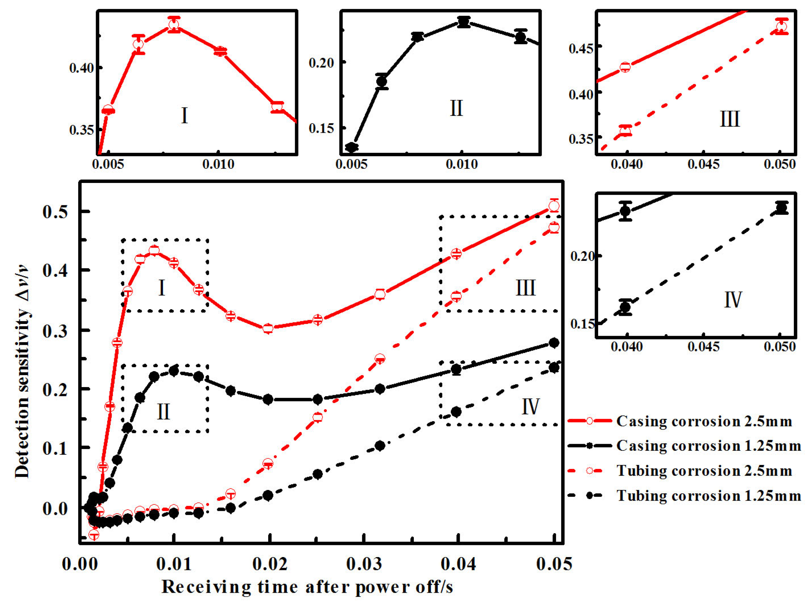
| Corrosion Depth | Tubing Corroding 1.25 mm | Tubing Corroding 2.5 mm | Casing Corroding 1.25 mm | Casing Corroding 2.5 mm |
|---|---|---|---|---|
| Up to 5% moments (after power off) /s | 0.0040 (point N) | 0.0025 (point M) | 0.0250 (point P) | 0.0200 (point O) |
| Up to 5% moments (absolute value) /s | 0.0665 | 0.0650 | 0.0875 | 0.0825 |
| Peak time (after power off) /s | 0.0100 s (point R) | 0.0080 (point Q) | 0.0625 (end) | 0.0625 (end) |
| Peak time (absolute value) /s | 0.0725 | 0.0705 | 0.1250 | 0.1250 |
Disclaimer/Publisher’s Note: The statements, opinions and data contained in all publications are solely those of the individual author(s) and contributor(s) and not of MDPI and/or the editor(s). MDPI and/or the editor(s) disclaim responsibility for any injury to people or property resulting from any ideas, methods, instructions or products referred to in the content. |
© 2023 by the authors. Licensee MDPI, Basel, Switzerland. This article is an open access article distributed under the terms and conditions of the Creative Commons Attribution (CC BY) license (https://creativecommons.org/licenses/by/4.0/).
Share and Cite
Yu, X.; Zhu, Y.; Cao, Y.; Xiong, J. Time-Domain Numerical Simulation and Experimental Study on Pulsed Eddy Current Inspection of Tubing and Casing. Sensors 2023, 23, 1135. https://doi.org/10.3390/s23031135
Yu X, Zhu Y, Cao Y, Xiong J. Time-Domain Numerical Simulation and Experimental Study on Pulsed Eddy Current Inspection of Tubing and Casing. Sensors. 2023; 23(3):1135. https://doi.org/10.3390/s23031135
Chicago/Turabian StyleYu, Xingxing, Ying Zhu, Yan Cao, and Juan Xiong. 2023. "Time-Domain Numerical Simulation and Experimental Study on Pulsed Eddy Current Inspection of Tubing and Casing" Sensors 23, no. 3: 1135. https://doi.org/10.3390/s23031135