Figure 1.
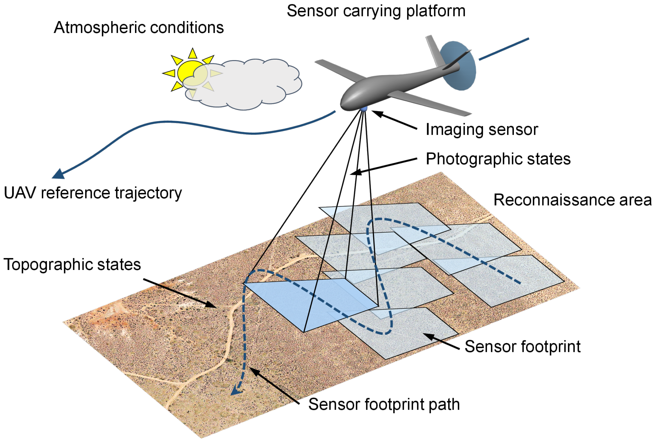
Illustration of relevant influencing factors on sensor-model-based trajectory optimization. Adapted from [
13].
Figure 1.
Illustration of relevant influencing factors on sensor-model-based trajectory optimization. Adapted from [
13].
Figure 2.
Principle of coverage path planning for a reconnaissance area (green). The sensor footprint path defines the positioning of the individual sensor footprints (pale blue). The size of the footprint is defined by and the Euclidean distance between footprints is determined by . The black dotted line marks the scanned area.
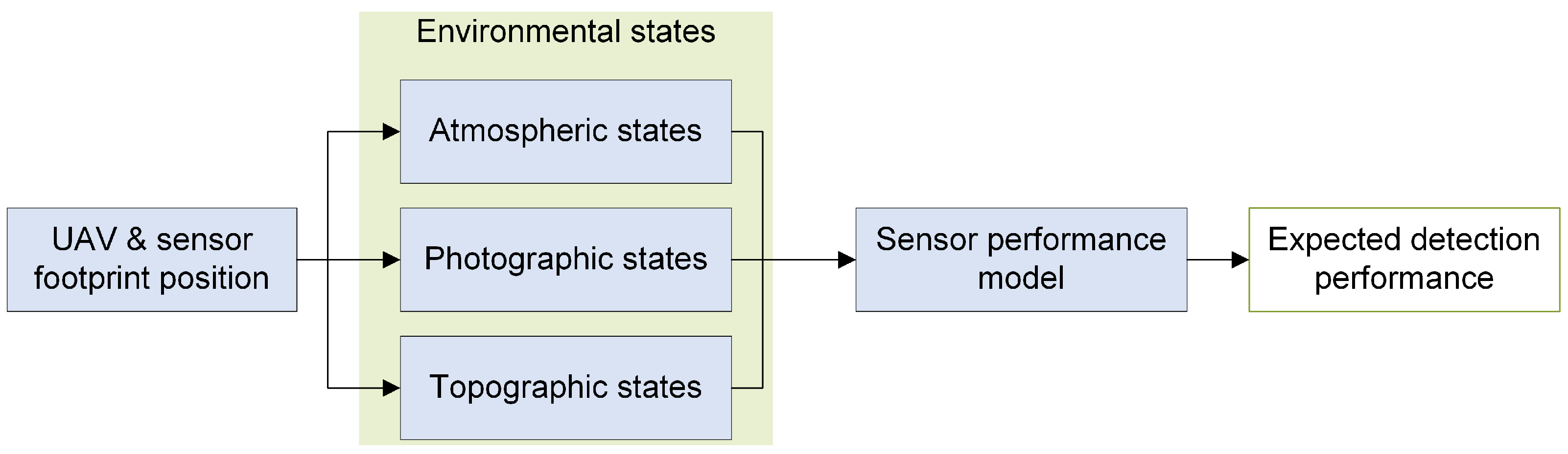
Figure 3.
The sensor performance model maps selected environmental states to the expected detection performance of a specific perception chain (not displayed). These environmental states comprise atmospheric, photographic, and topographic conditions resulting from the positioning of the UAV and the sensor footprint on the ground.
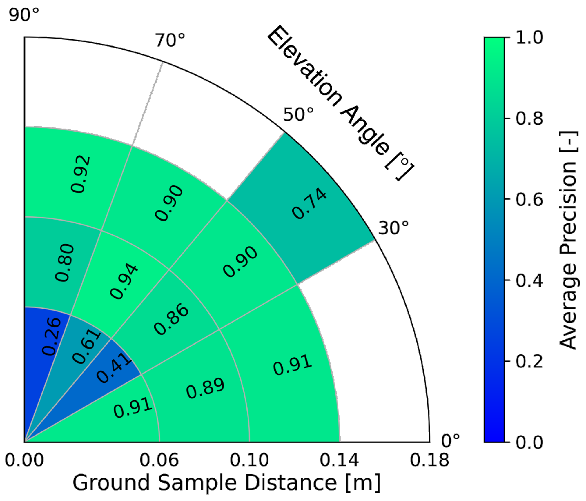
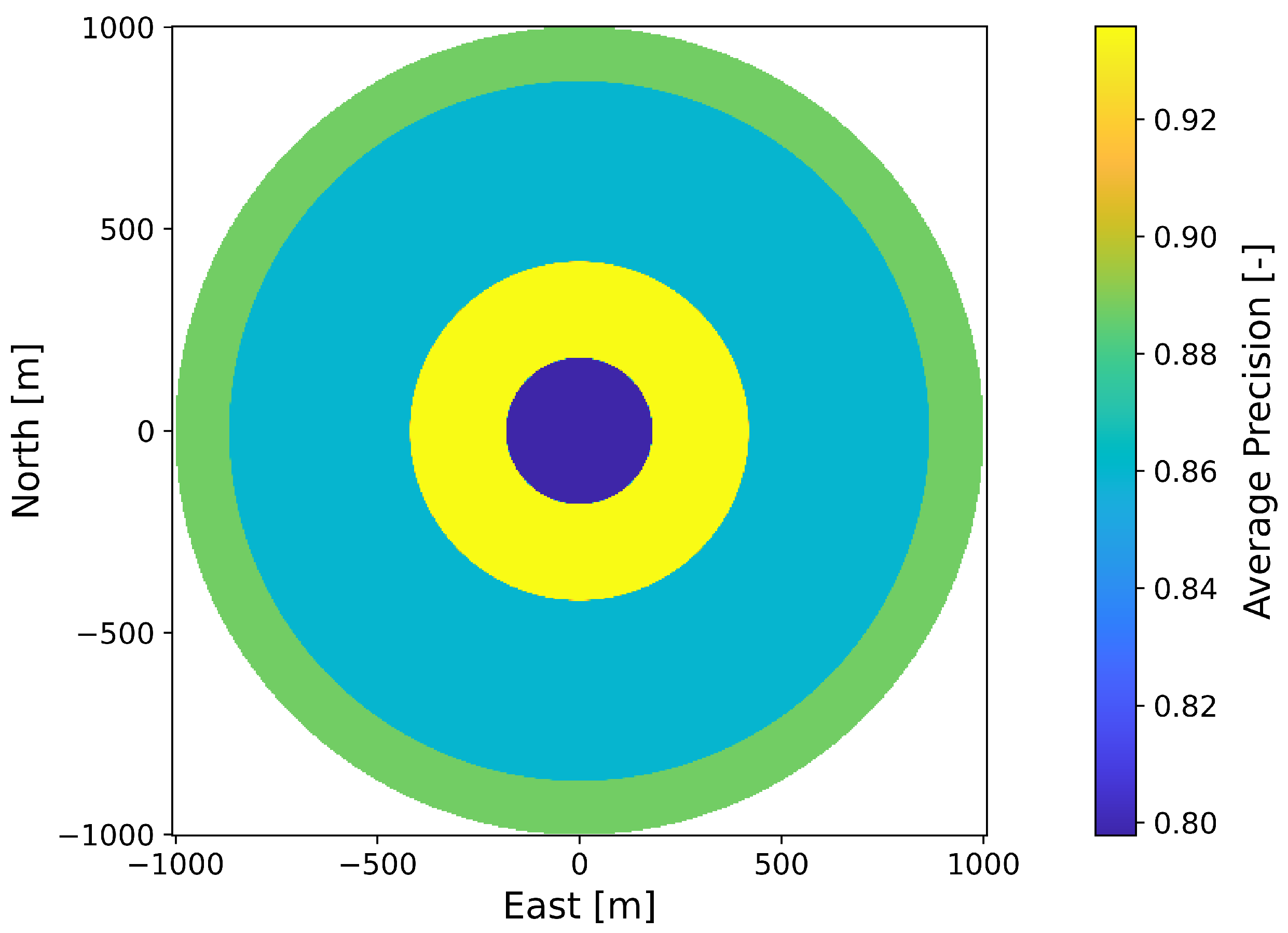
Figure 5.
Illustration of the average precision (color-coded) for different interval ranges of the ground sample distance and the elevation angle corresponding to a specific composition of the environmental state.
Figure 5.
Illustration of the average precision (color-coded) for different interval ranges of the ground sample distance and the elevation angle corresponding to a specific composition of the environmental state.
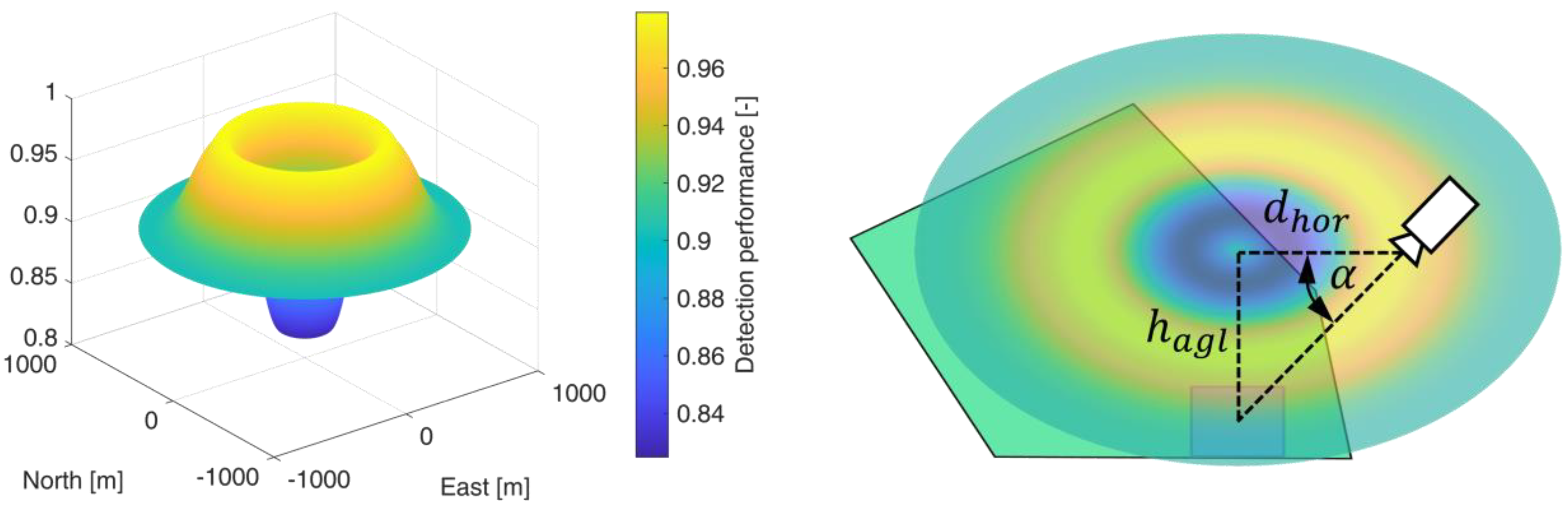
Figure 6.
Representation of a perception map from the CC sensor performance model as a 3-dimensional plot (left) and the same map in a planar representation (right), with reference to the corresponding sensor footprint (pale blue square) on the ground. The elevation angle is determined by the horizontal distance and the altitude above ground . The color-coding of the perception map corresponds to the predicted detection performance. Light colors represent high performance values, while darker colors correlate with lower values.
Figure 7.
Perception map resulting from the Yolo-SPM sensor performance model.
Figure 7.
Perception map resulting from the Yolo-SPM sensor performance model.
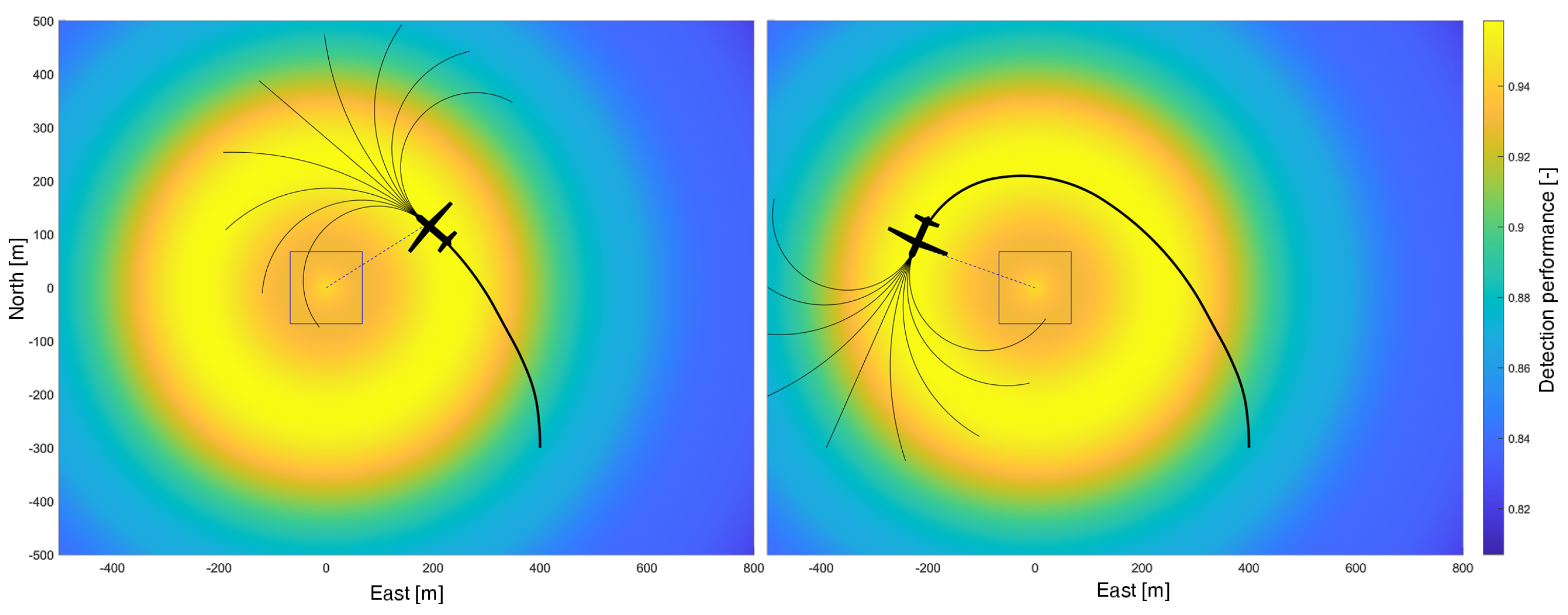
Figure 8.
Depiction of the principle of path planning. The fan-shaped path array consists (for representational reasons) of 9 evenly spaced curves (thin black lines). The thick black line is the resulting UAV trajectory from trajectory optimization. The square represents the sensor footprint on the ground. The perception map, which results from atmospheric and topographic conditions is color-coded. Yellow areas mark regions with high detection performance. Adapted from [
13].
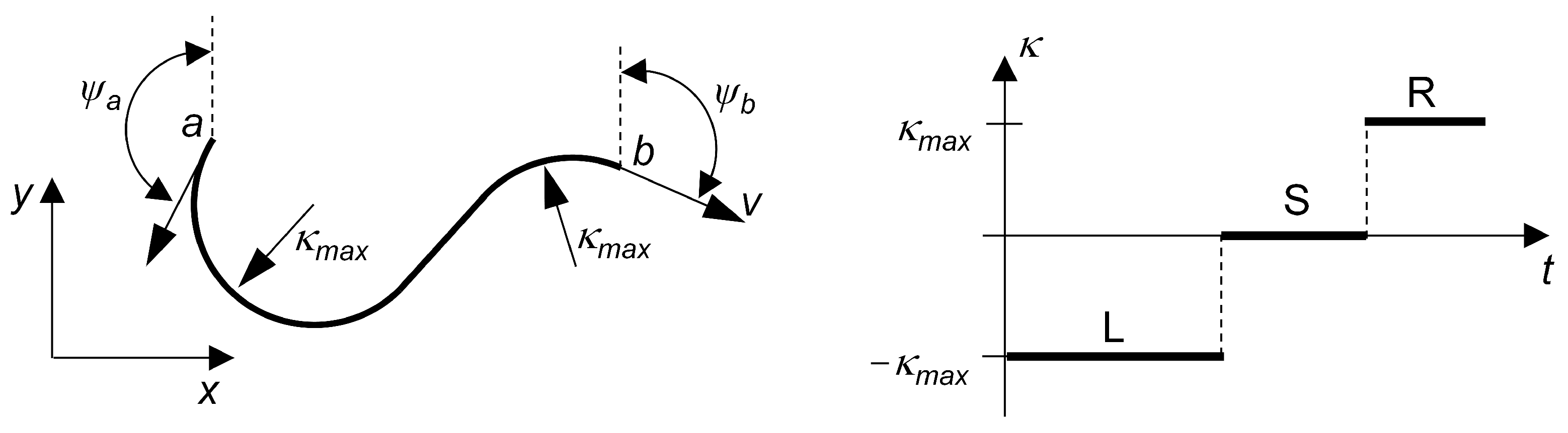
Figure 9.
Example of a Dubins path from the start configuration a to the goal configuration b defined by a specific set of motion primitives L, S and R (left). The associated curvature profile of the Dubins path is plotted on the (right).
Figure 9.
Example of a Dubins path from the start configuration a to the goal configuration b defined by a specific set of motion primitives L, S and R (left). The associated curvature profile of the Dubins path is plotted on the (right).
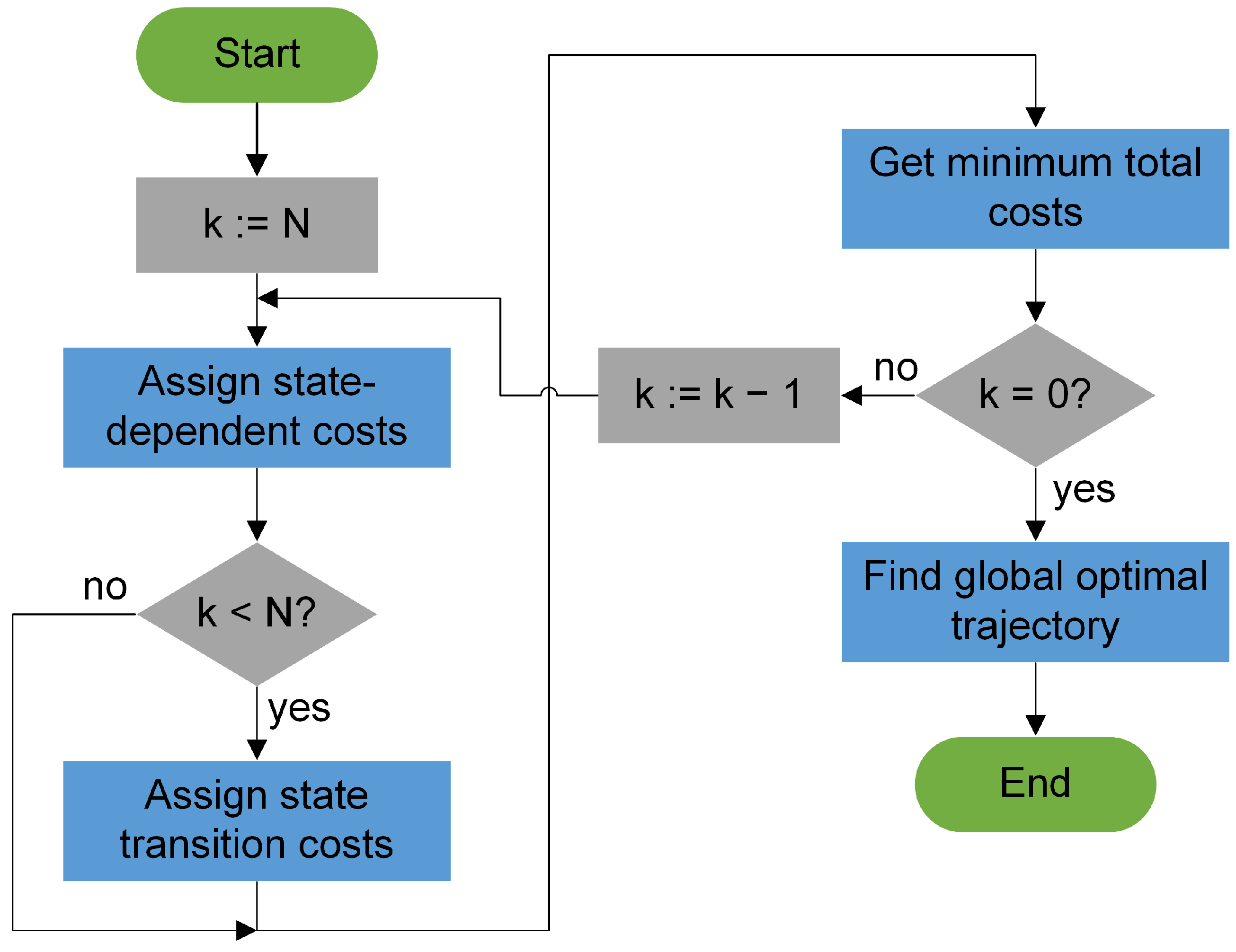
Figure 10.
Flow chart of the DP&OC process for time steps , N.
Figure 10.
Flow chart of the DP&OC process for time steps , N.
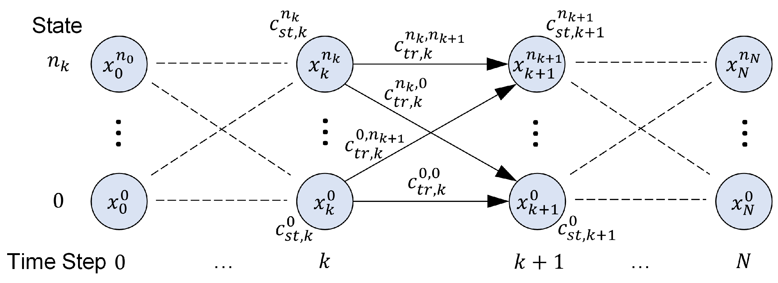
Figure 11.
Illustration of the states and the state transitions in an acyclic graph. Circles represent the states in the individual time steps . The arrows represent the state transitions between two states. As an example, the state-dependent costs and the state transition costs are plotted from time step k to .
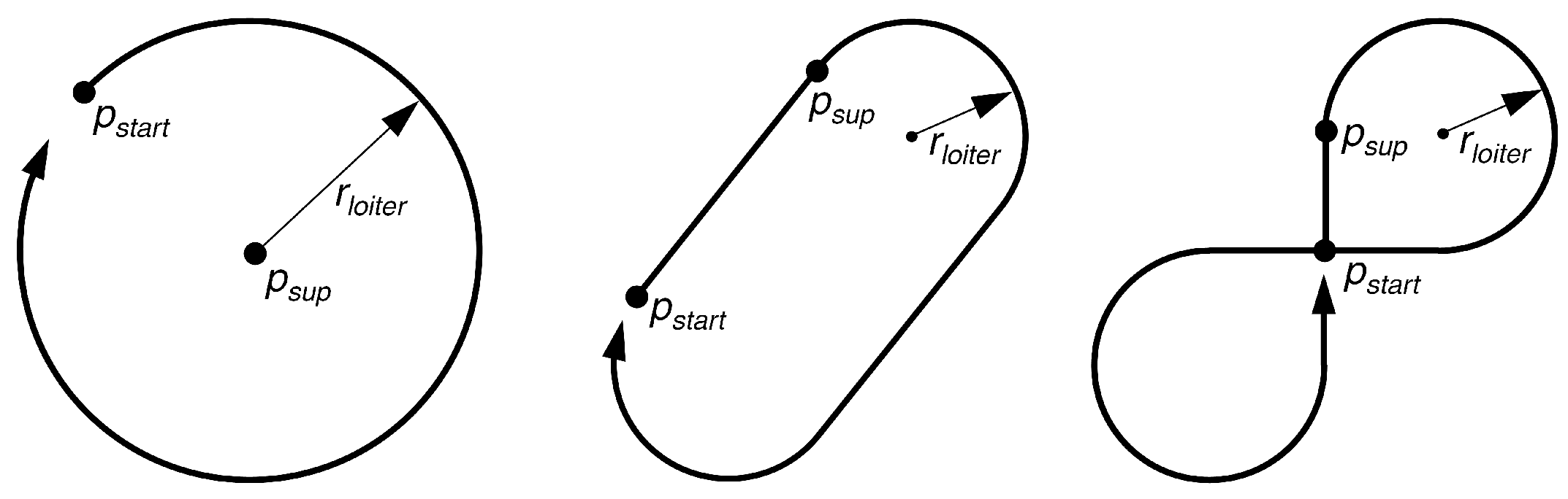
Figure 12.
Illustration of the benchmark trajectories Circle (left), Racetrack (center) and Figure-8 (right). Additionally, the starting point , the support point and the path direction are sketched. The radius is predefined or results from the design.
Figure 12.
Illustration of the benchmark trajectories Circle (left), Racetrack (center) and Figure-8 (right). Additionally, the starting point , the support point and the path direction are sketched. The radius is predefined or results from the design.
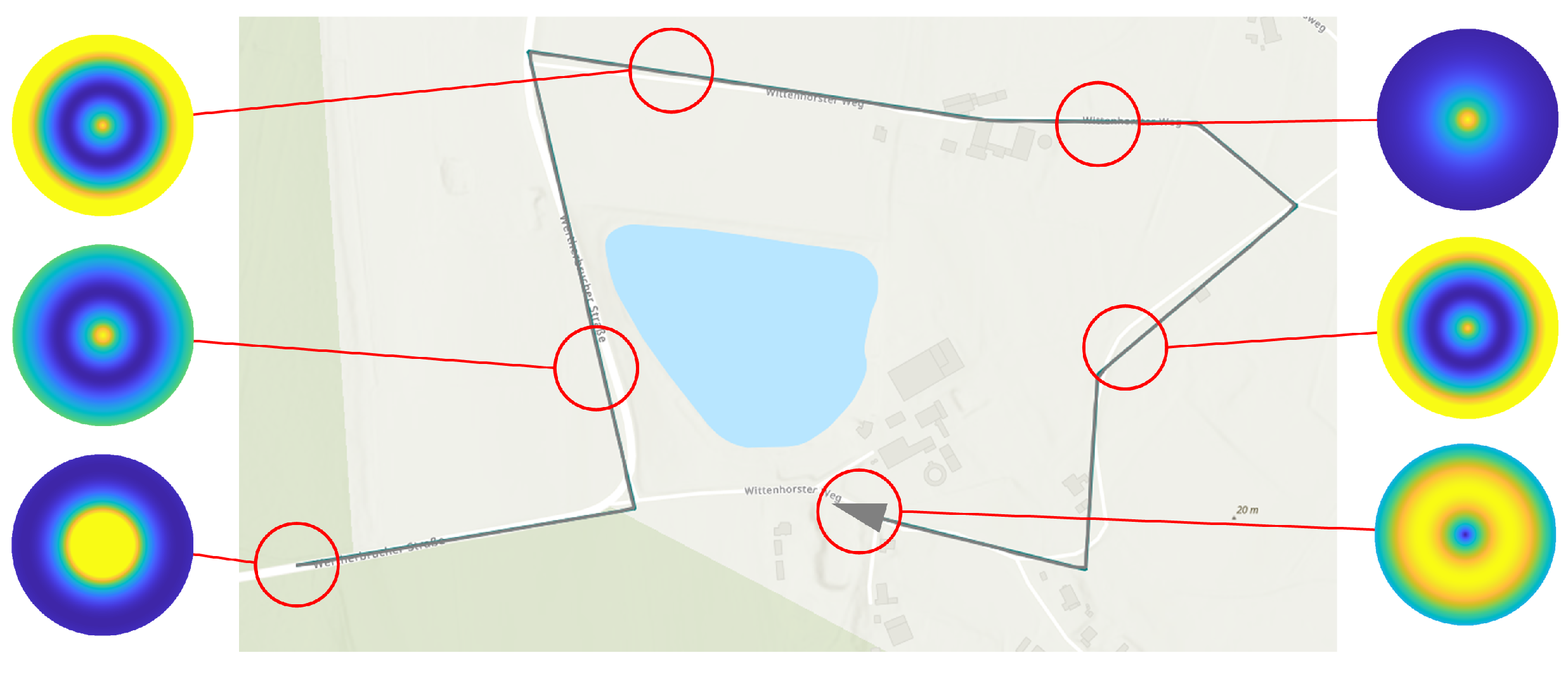
Figure 13.
Illustration of the route reconnaissance scenario. The green line marks the reconnaissance route, supplemented by several perception maps resulting from the CC-SPM performance model. The color-coding of the different perception maps corresponds to the predicted detection performance. Light colors represent high performance values, while darker colors correlate with lower values.
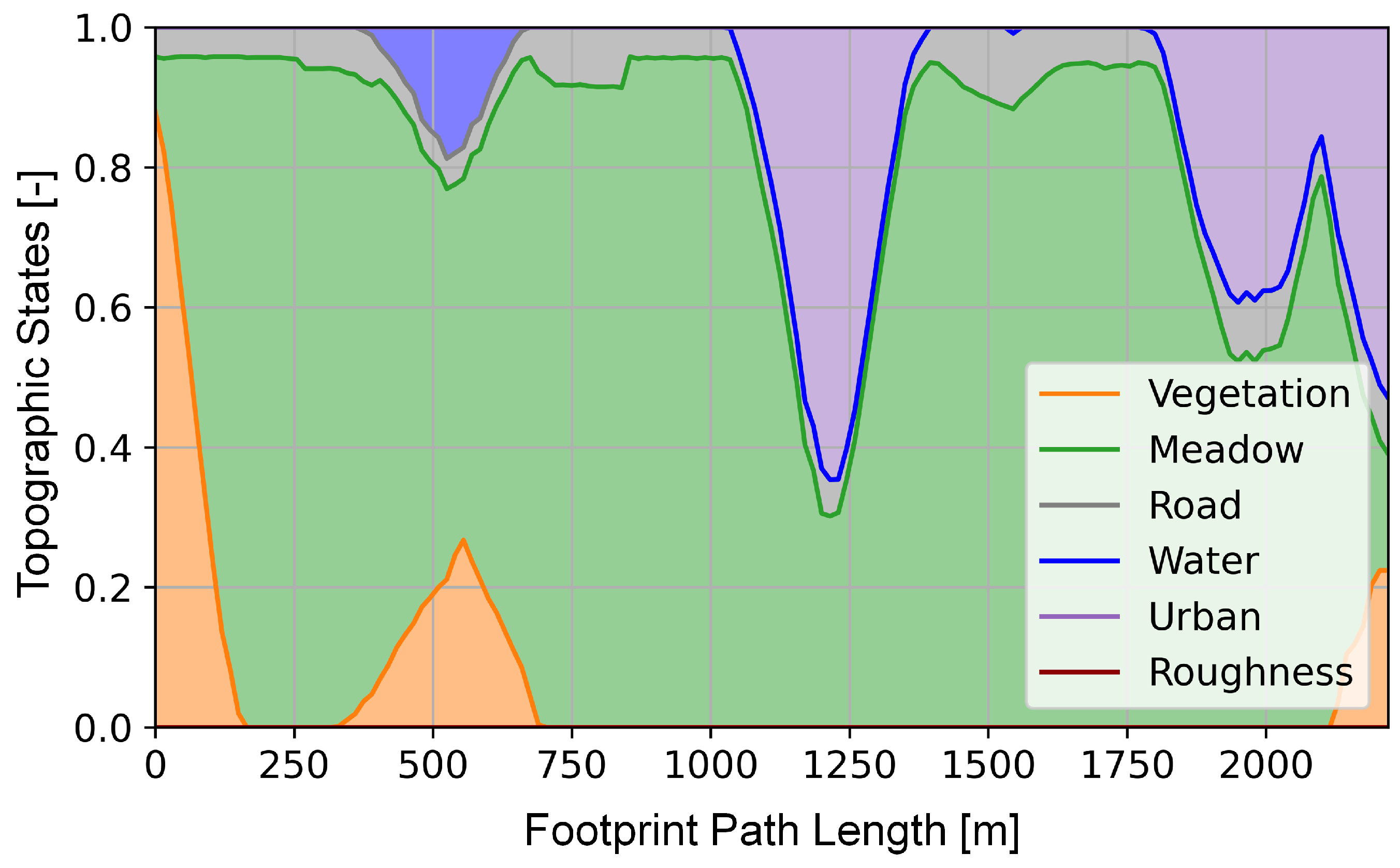
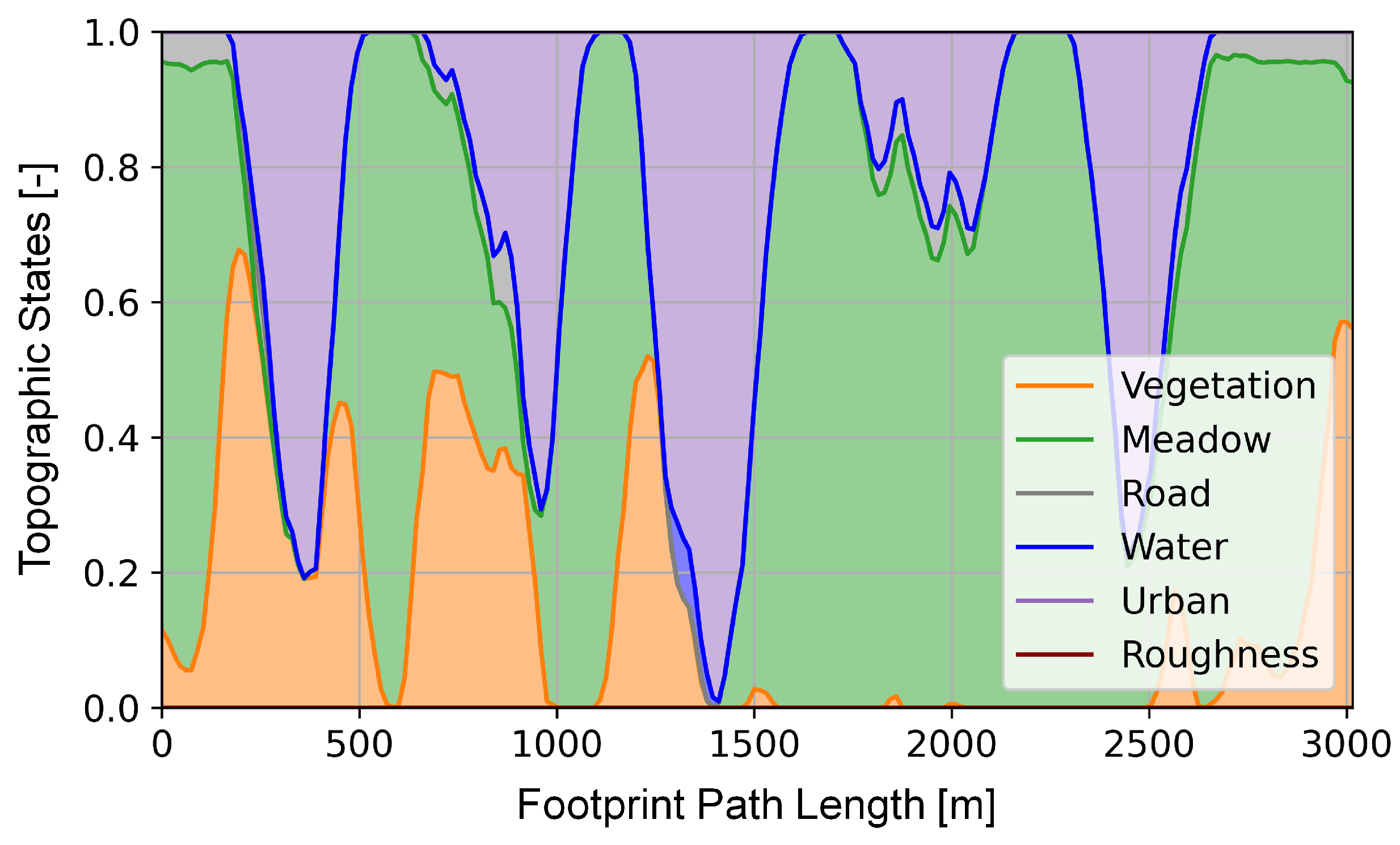
Figure 14.
Topographic states resulting from the route reconnaissance scenario.
Figure 14.
Topographic states resulting from the route reconnaissance scenario.
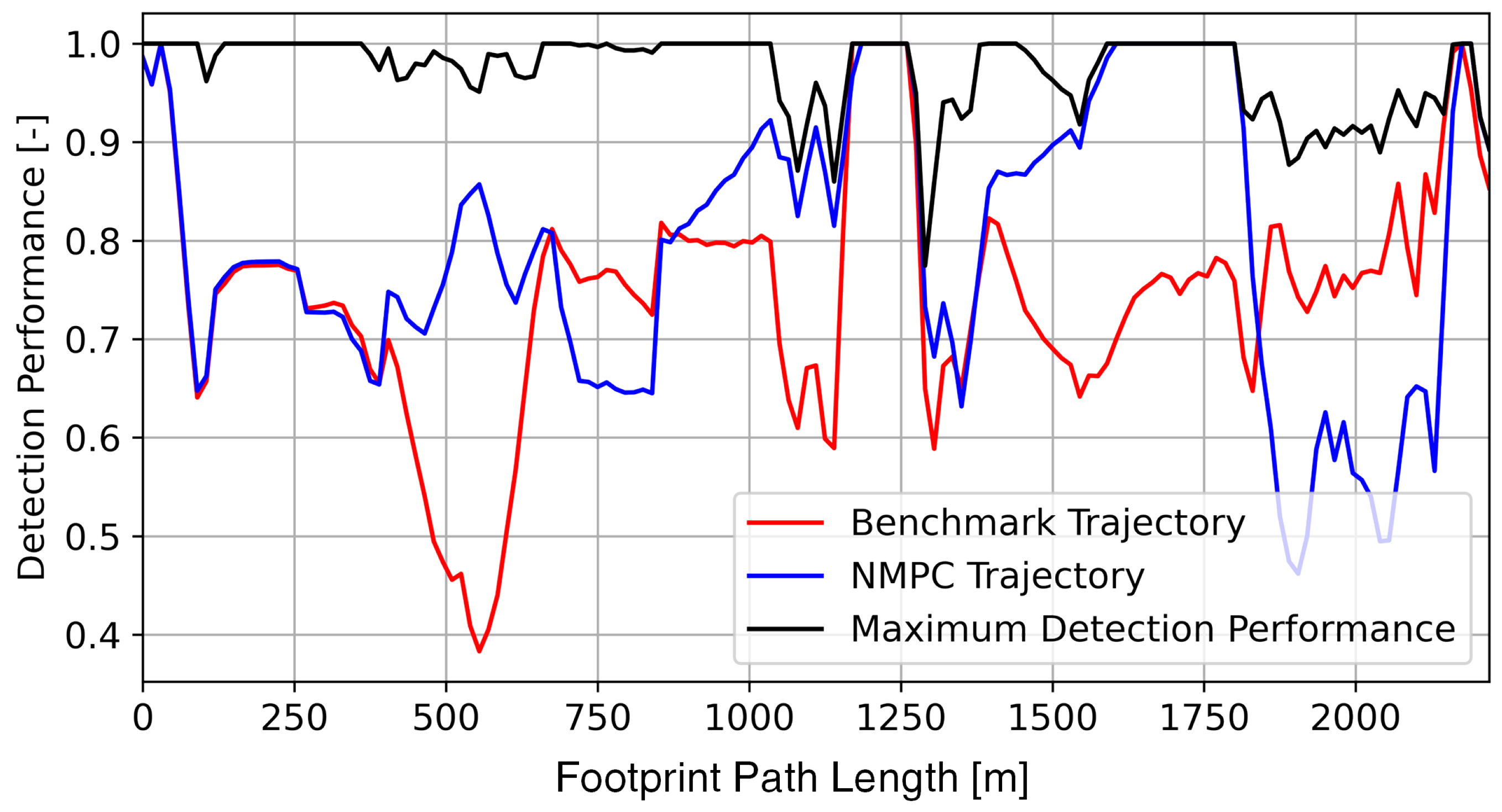
Figure 15.
Illustration of the detection performances for the NMPC and benchmark trajectory with respect to the sensor footprint path length. The black line marks the theoretical maximum detection performance as an upper bound.
Figure 15.
Illustration of the detection performances for the NMPC and benchmark trajectory with respect to the sensor footprint path length. The black line marks the theoretical maximum detection performance as an upper bound.
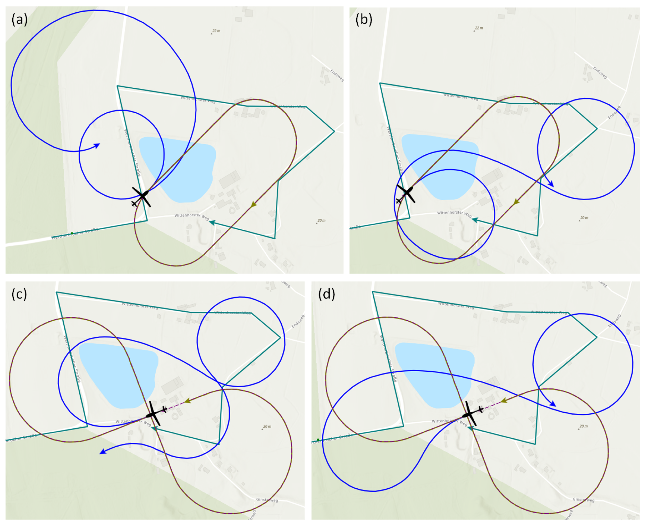
Figure 16.
Trajectory optimization for the route reconnaissance scenario with sensor performance model CC-SPM in (a,c) and with Yolo-SPM in (b,d). The blue line indicates the NMPC-optimized reference trajectory and the light green line represents the benchmark trajectory. The starting points of both trajectories are identical and marked by a black aircraft symbol. In (a,b), the Racetrack benchmark pattern is displayed, whereas in (c,d), the Figure-8 pattern is applied.
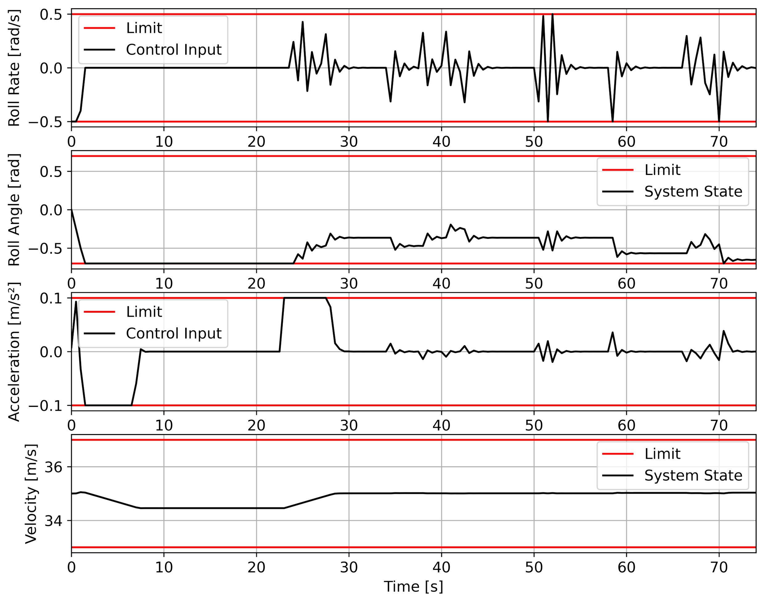
Figure 17.
Illustration of the control inputs “roll rate” and “acceleration” for route reconnaissance with CC-SPM, plotted with respect to the flight duration. The control inputs yield changes in the system states “velocity” and “roll angle”. Shown also are the predefined limitations.
Figure 17.
Illustration of the control inputs “roll rate” and “acceleration” for route reconnaissance with CC-SPM, plotted with respect to the flight duration. The control inputs yield changes in the system states “velocity” and “roll angle”. Shown also are the predefined limitations.
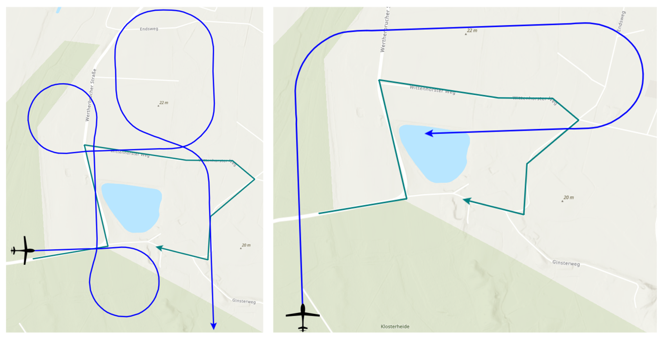
Figure 18.
Depiction of the DP&OC-optimized trajectories for the route reconnaissance scenario with sensor performance models CC-SPM (left) and Yolo-SPM (right). The blue line marks the UAV flight trajectory and the green line maps the sensor footprint on the ground.
Figure 18.
Depiction of the DP&OC-optimized trajectories for the route reconnaissance scenario with sensor performance models CC-SPM (left) and Yolo-SPM (right). The blue line marks the UAV flight trajectory and the green line maps the sensor footprint on the ground.
Figure 19.
Illustration of the area reconnaissance scenario. The green line marks the sensor footprint path within the green reconnaissance area. Several perception maps resulting from the CC-SPM model illustrate the detection performance along the footprint path. The red lines indicate the positions of the perception maps along the sensor path. The color-coding of the different perception maps corresponds to the predicted detection performance.
Figure 20.
Topographic states resulting from the area reconnaissance scenario.
Figure 20.
Topographic states resulting from the area reconnaissance scenario.
Figure 21.
Trajectory optimization for the area reconnaissance scenario with sensor performance model CC-SPM in (a,c) and with Yolo-SPM in (b,d). The blue line indicates the NMPC-optimized reference trajectory and the light green line marks the benchmark trajectory. The starting points of both trajectories are identical and depicted by the aircraft symbol. In (a,b), the Figure-8 pattern is used, whereas in (c,d), the Circle benchmark pattern is applied.
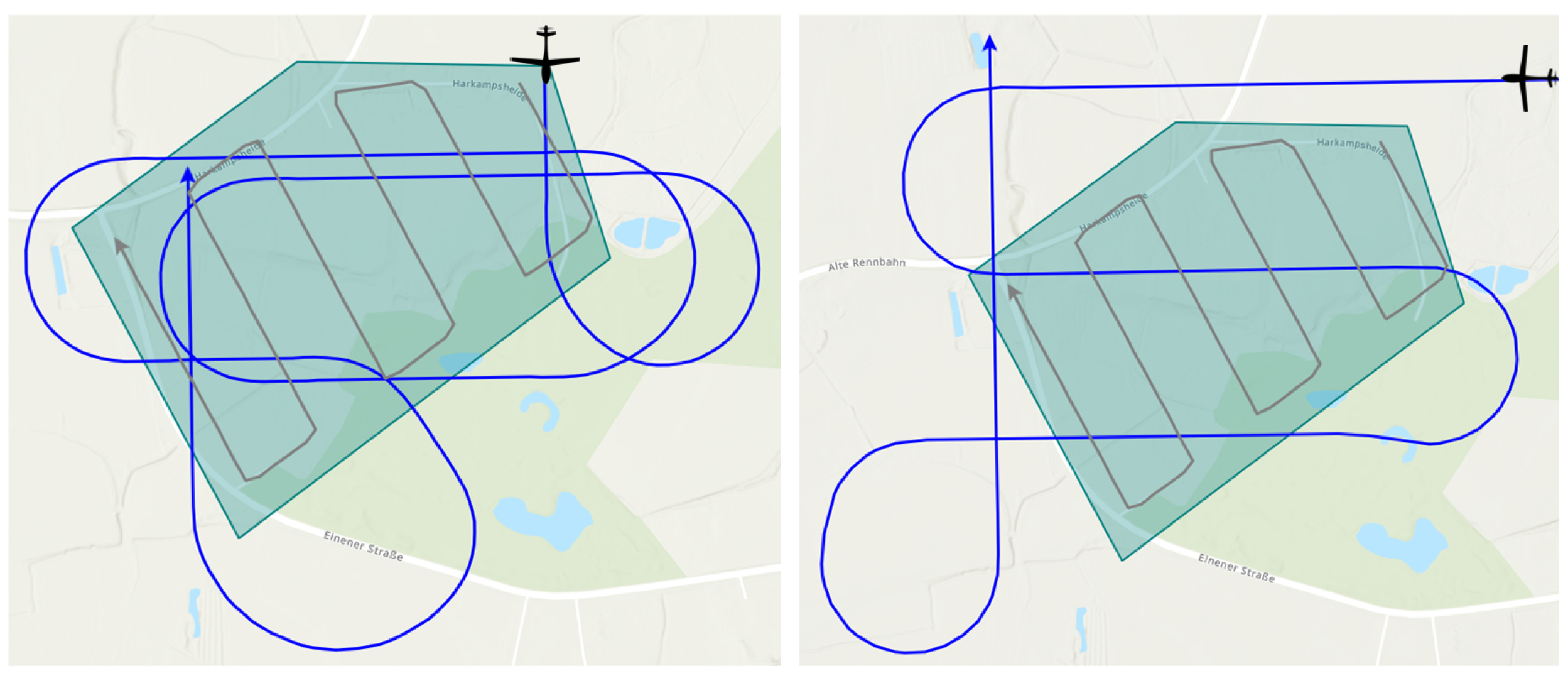
Figure 22.
Illustration of the DP&OC-optimized trajectories for the area reconnaissance scenario with sensor performance models CC-SPM (left) and Yolo-SPM (right). The blue line depicts the UAV flight trajectory and the green line marks the sensor footprint on the ground.
Figure 22.
Illustration of the DP&OC-optimized trajectories for the area reconnaissance scenario with sensor performance models CC-SPM (left) and Yolo-SPM (right). The blue line depicts the UAV flight trajectory and the green line marks the sensor footprint on the ground.
Table 1.
Parameter settings for coverage path planning.
Table 1.
Parameter settings for coverage path planning.
| Parameter | Setting | Remark |
|---|
| target ground sample distance | 0.07 m | predefined |
| sensor resolution | 1920 px | predefined |
| sweep width | 134.4 m | from Equation (1) |
| footprint velocity | 30 m/s | predefined |
| time step interval | 0.5 s | predefined |
| distance | 15 m | from Equation (2) |
Table 2.
Atmospheric states comprising the aerial imagery dataset of [
36].
Table 2.
Atmospheric states comprising the aerial imagery dataset of [
36].
| Environmental State | Attributes |
|---|
| season | summer, autumn |
| daytime | day, night |
| visibility | clear, foggy |
| road condition | wet, dry |
| sky cover | covered, sunny |
Table 3.
Parameter settings for the generation of the perception maps.
Table 3.
Parameter settings for the generation of the perception maps.
| Parameter | Setting | Remark |
|---|
| UAV altitude above ground | 500 m | predefined |
| perception map diameter | 2000 m | predefined |
Table 4.
Parameter settings for the path planning process.
Table 4.
Parameter settings for the path planning process.
| Parameter | Setting | Remark |
|---|
| preview horizon time steps | 25 | predefined |
| time step interval | 0.5 s | from Table 1 |
| uav setpoint velocity | 35 m/s | predefined |
| path length | 437.5 m | from Equation (13) |
| number of paths Z | 15 | predefined |
Table 5.
Parameter settings for nonlinear model predictive control.
Table 5.
Parameter settings for nonlinear model predictive control.
| Parameter | Setting | Remark |
|---|
| prediction horizon N | 10 | predefined |
| maximum roll angle | 0.7 rad | from Equation (18) |
| setpoint roll angle | 0 rad | predefined |
| maximum roll rate | 0.5 rad/s | from Equation (19) |
| setpoint roll rate | 0 rad/s | predefined |
| minimum velocity | 33 m/s | from Equation (21) |
| maximum velocity | 37 m/s | from Equation (21) |
| setpoint velocity | 35 m/s | predefined |
| maximum acceleration | 0.1 | from Equation (20) |
| setpoint acceleration | 0 | predefined |
| diagonal weighting matrix Q | 1, 1, 0.1, 0.1, 0.1 | predefined |
| diagonal weighting matrix R | 0.5, 0.5 | predefined |
Table 6.
Parameter settings for the combined path planning and NMPC.
Table 6.
Parameter settings for the combined path planning and NMPC.
| Parameter | Setting | Remark |
|---|
| weighting factor | 0.8 | predefined |
Table 7.
Parameter settings for Dubins path planning.
Table 7.
Parameter settings for Dubins path planning.
| Parameter | Setting | Remark |
|---|
| UAV velocity v | 35 m/s | predefined |
| maximum roll angle | 0.694 rad | predefined |
| gravitational acceleration g | 9.81 | |
| minimum turn radius | 150 m | from Equation (35) |
Table 8.
Parameter settings for dynamic programming and optimal control.
Table 8.
Parameter settings for dynamic programming and optimal control.
| Parameter | Setting | Remark |
|---|
| UAV velocity v | 35 m/s | from Table 7 |
| minimum turn radius | 150 m | from Table 7 |
| time step interval | 0.5 s | from Table 1 |
| minimum Dubins path length | 17.5 m | from Equation (44) |
| maximum Dubins path length | 942.5 m | from Equation (45) |
| weighting factor | 0.5 | predefined |
| number of yaw angles | 12 | predefined |
Table 9.
Parameter settings of the atmospheric conditions for the CC-SPM sensor performance model.
Table 9.
Parameter settings of the atmospheric conditions for the CC-SPM sensor performance model.
| Parameter | Setting | Remark |
|---|
| time of day | 16 h | predefined |
| month | June | predefined |
| cloud cover | 25% | predefined |
| fog density | 0% | predefined |
| precipitation | 0% | predefined |
Table 10.
Parameter settings of the atmospheric conditions for the Yolo-SPM sensor performance model.
Table 10.
Parameter settings of the atmospheric conditions for the Yolo-SPM sensor performance model.
| Parameter | Setting | Remark |
|---|
| daytime | day | predefined |
| season | autumn | predefined |
| visibility | clear | predefined |
| road condition | wet | predefined |
| sky cover | covered | predefined |
Table 11.
Predicted detection performance results for route reconnaissance with NMPC optimization.
Table 11.
Predicted detection performance results for route reconnaissance with NMPC optimization.
| | CC-SPM | Yolo-SPM |
|---|
| | NMPC | Benchm. | NMPC | Benchm. |
|---|
| maximum average detection performance | 0.972 | 0.972 | 0.936 | 0.936 |
| average detection performance (abs.) | 0.815 | 0.772 | 0.924 | 0.878 |
| average detection performance (rel.) | 83.88% | 79.42% | 98.66% | 93.77% |
Table 12.
Predicted detection performance results for route reconnaissance with DP&OC optimization.
Table 12.
Predicted detection performance results for route reconnaissance with DP&OC optimization.
| | CC-SPM | Yolo-SPM |
|---|
| maximum average detection performance | 0.972 | 0.936 |
| average detection performance (abs.) | 0.910 | 0.936 |
| average detection performance (rel.) | 93.62% | 100.00% |
Table 13.
Predicted detection performance results for area reconnaissance with NMPC optimization.
Table 13.
Predicted detection performance results for area reconnaissance with NMPC optimization.
| | CC-SPM | Yolo-SPM |
|---|
| | NMPC | Benchm. | NMPC | Benchm. |
|---|
| maximum average detection performance | 0.948 | 0.948 | 0.936 | 0.936 |
| average detection performance (abs.) | 0.846 | 0.810 | 0.933 | 0.887 |
| average detection performance (rel.) | 89.19% | 85.48% | 99.66% | 94.80% |
Table 14.
Predicted detection performance results for area reconnaissance with DP&OC optimization.
Table 14.
Predicted detection performance results for area reconnaissance with DP&OC optimization.
| | CC-SPM | Yolo-SPM |
|---|
| maximum average detection performance | 0.948 | 0.936 |
| average detection performance (abs.) | 0.909 | 0.936 |
| average detection performance (rel.) | 95.89% | 100.00% |


