
End-to-End Bubble Size Distribution Detection Technique in Dense Bubbly Flows Based on You Only Look Once Architecture


Abstract
:1. Introduction
2. Methodology
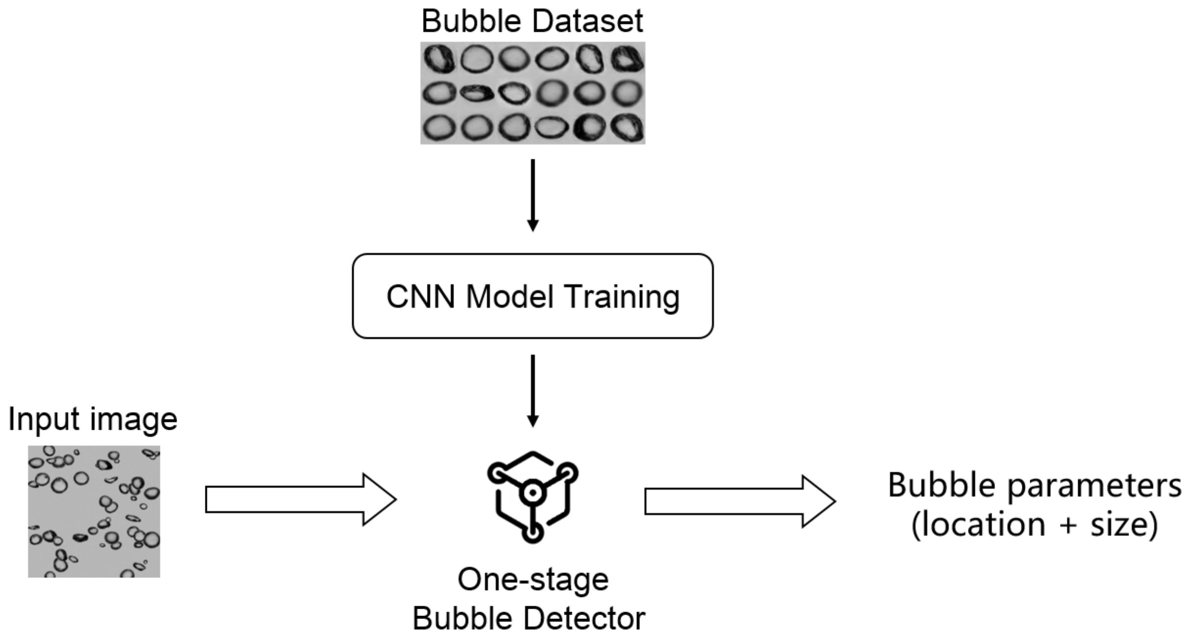
2.1. Overview
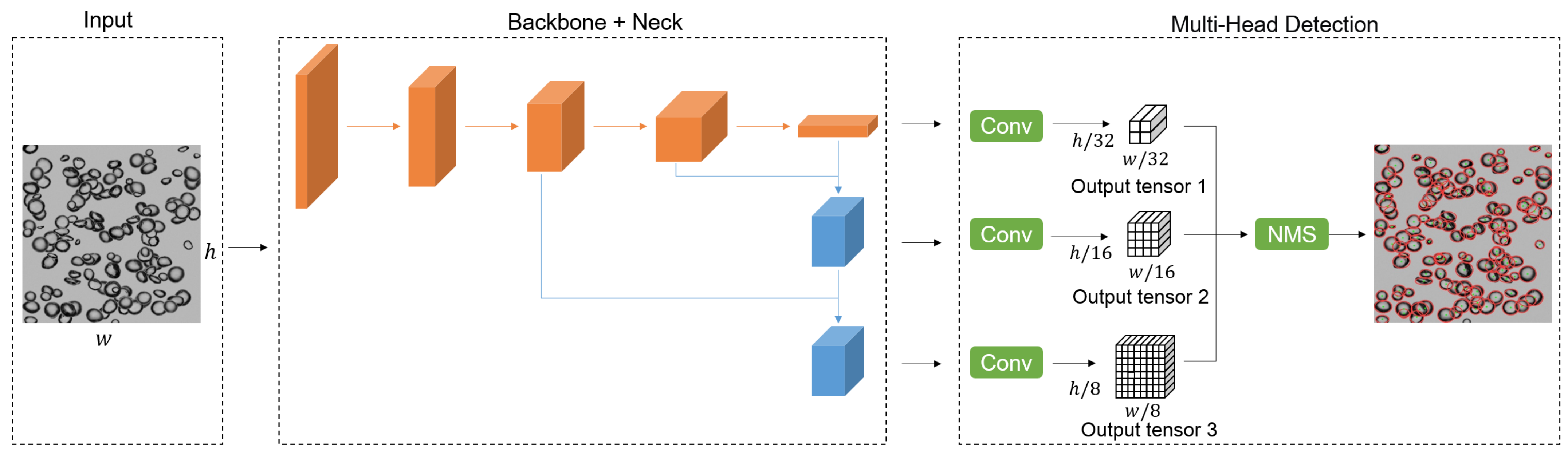
2.2. BSD Detector Architecture
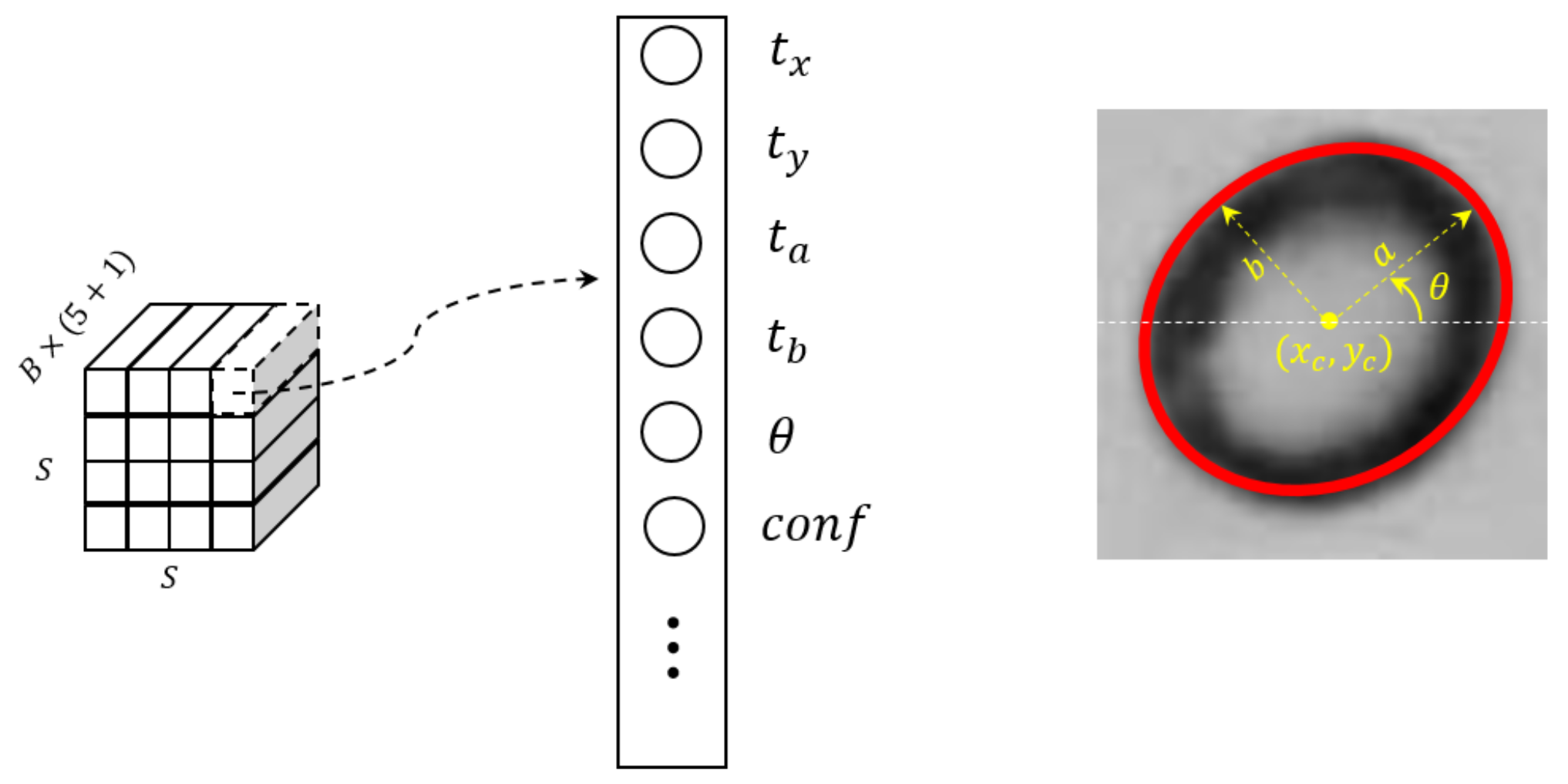
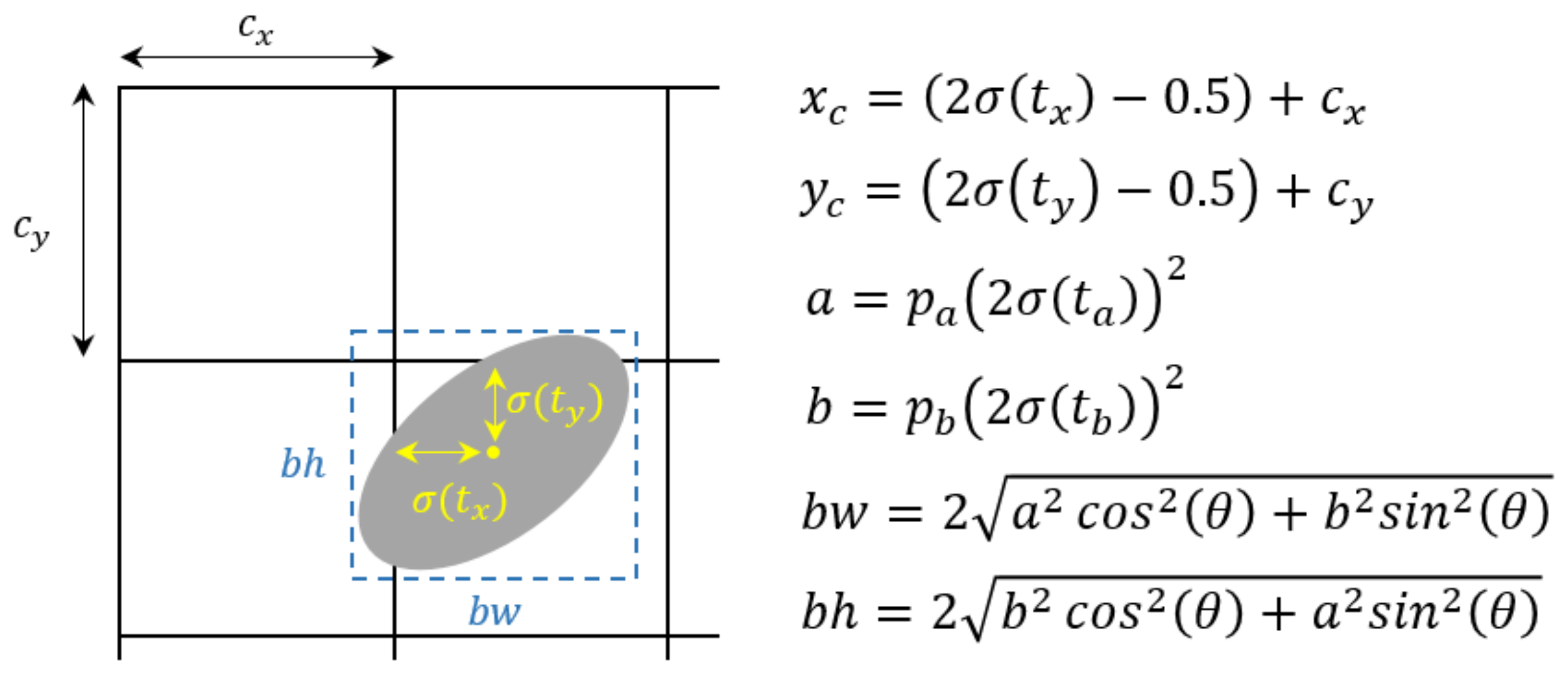
2.3. Ellipse Location and Fitting
2.4. Loss Function Design
3. Experiments
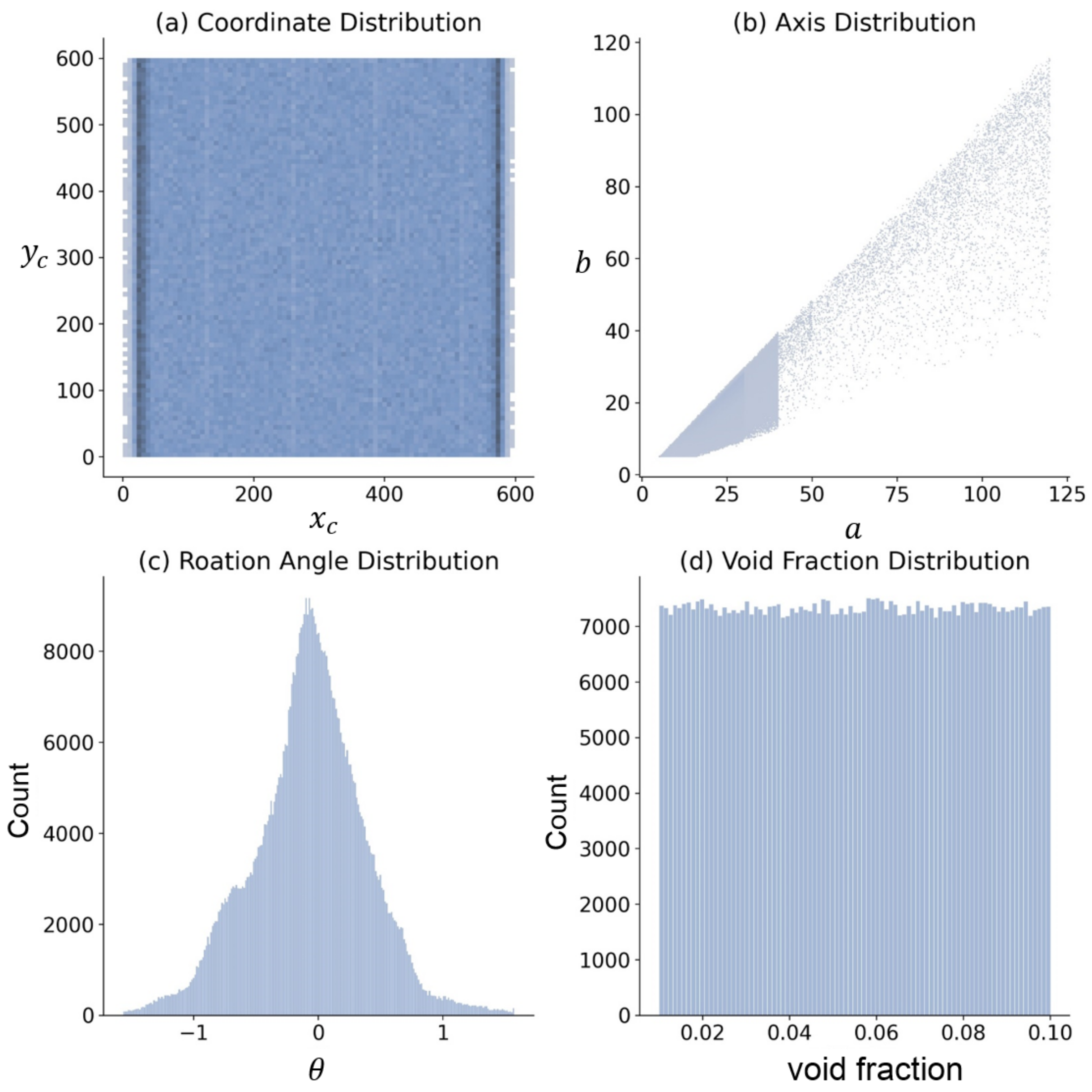
3.1. Dataset
3.2. Evaluation Metrics
- (1)
- Precision: The fraction of relevant instances among the retrieved instances
- (2)
- Recall: The fraction of relevant instances that were retrieved
- (3)
- AP50: the average precision (AP) value calculated at the threshold of 50% for detection evaluation. Specially, average precision is equivalent to mean average precision (mAP) due to a single-class detection task.
- (4)
- F1 score: A harmonic average of precision and recall
- (5)
- MSE: Average squared difference between the estimated values and the actual value.where M is the number of true positive samples, are the predicted values, and are the true values.
- (6)
- Frames Per Second (FPS): the frequency (rate) at which consecutive images (frames) are inferred
- (7)
- FLOPs: Floating point operations to measure the complexity of the CNN model.
3.3. Analysis of Backbone Networks
3.4. Analysis of Loss Function and IoU
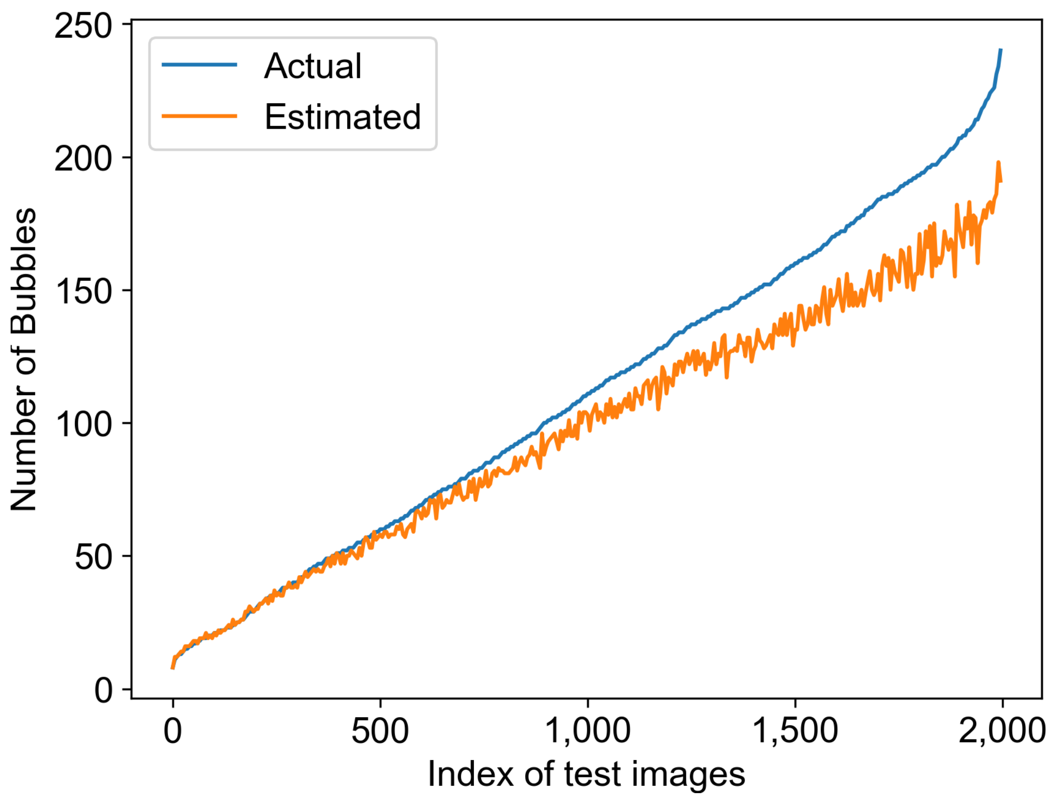
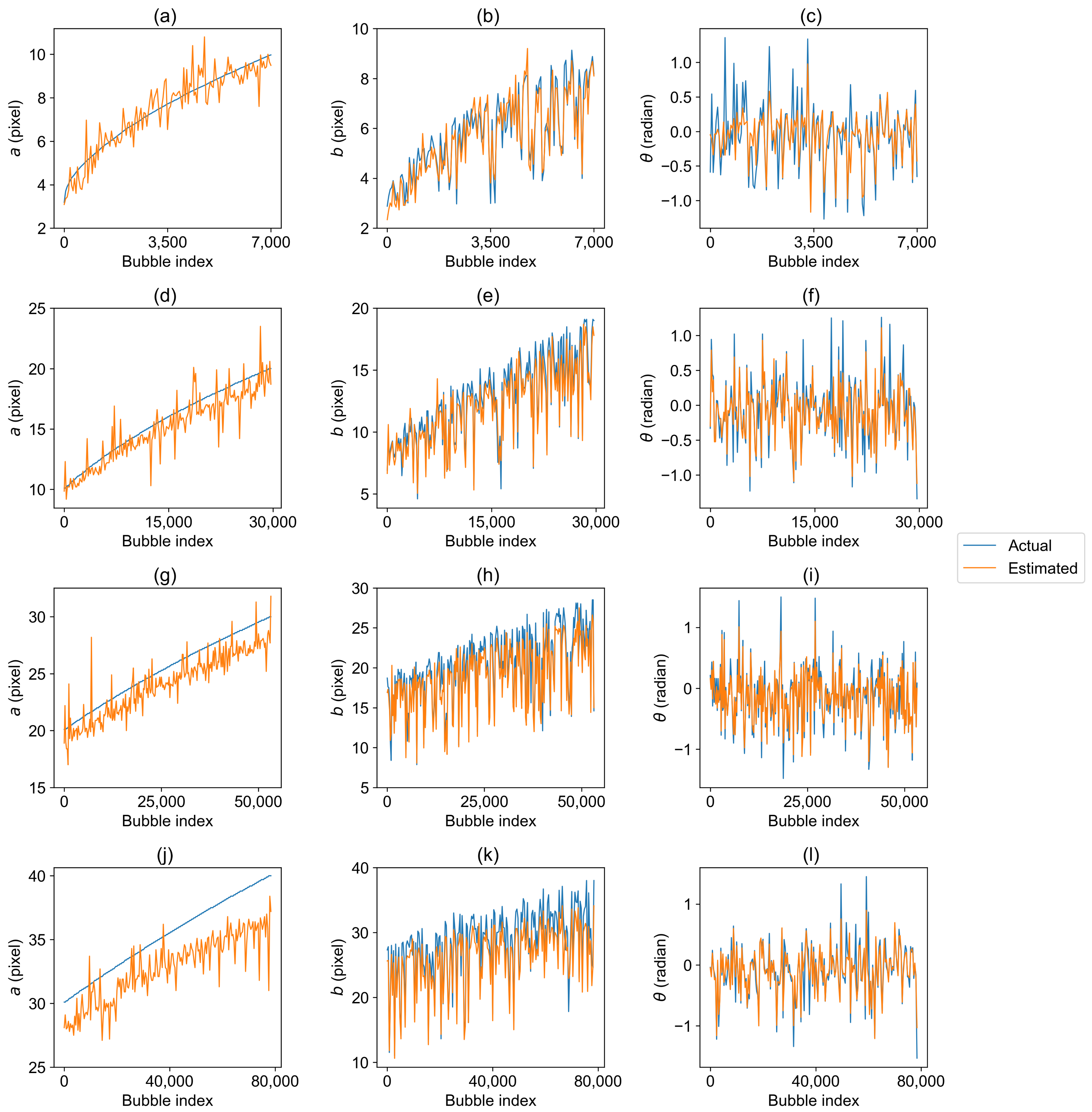
3.5. Bubble Size Distribution Estimation Evaluation
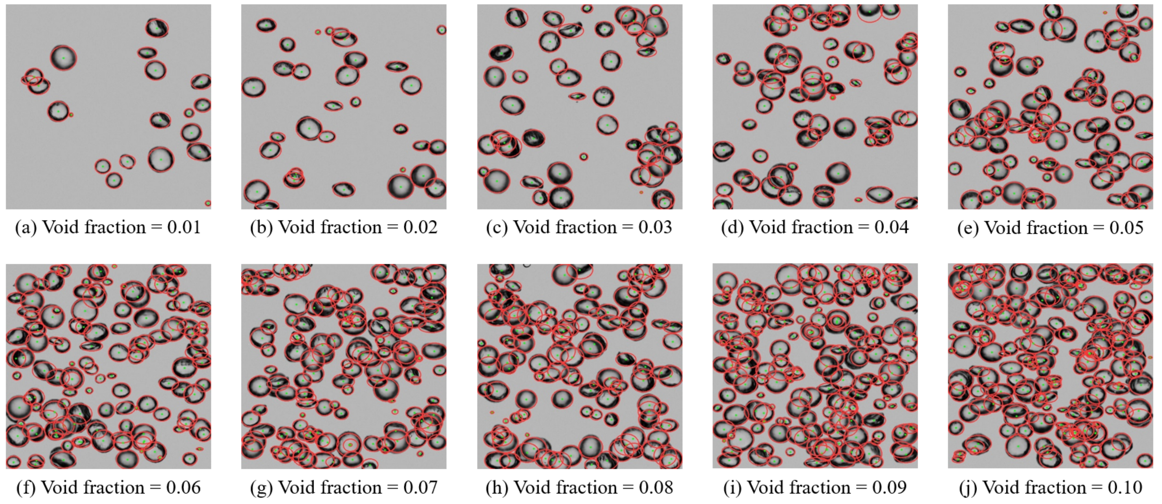
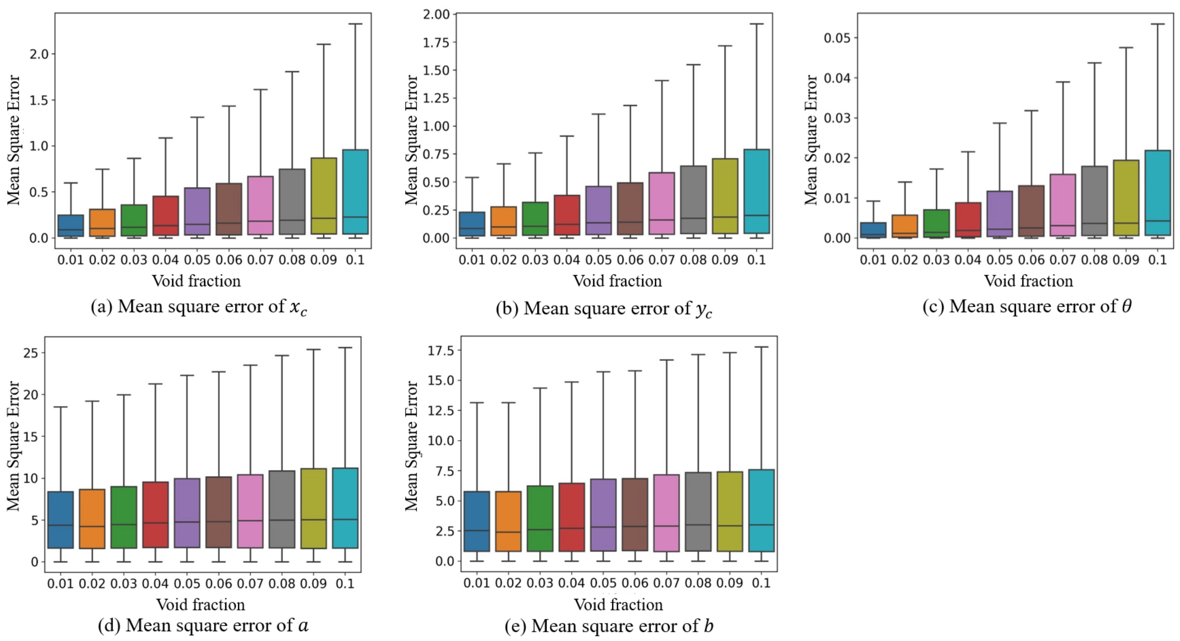
3.6. Analysis under Different Void Fractions
4. Discussions
5. Conclusions
- (1)
- An end-to-end BSD detection method based on YOLO is proposed, using a multi-head detection method to detect different-sized bubbles from three scales, and detecting dense objects by using a dense detection approach. The model also adds an ellipse fitting output for the morphological parameters of the bubbles, achieving a synchronous output of their position and position parameters.
- (2)
- The loss function of dense bubble detection is optimized using CIoU of bubble objects and constraints of elliptical parameters to improve the accuracy of model parameter fitting. The precision, recall, and AP50 of the model are 0.9871, 0.8725, and 0.9161 respectively, and the MSE of the parameters is 3.8299.
Author Contributions
Funding
Institutional Review Board Statement
Informed Consent Statement
Data Availability Statement
Acknowledgments
Conflicts of Interest
References
- Peng, C.; Liu, Y.; Gui, W.; Tang, Z.; Chen, Q. Bubble image segmentation based on a novel watershed algorithm with an optimized mark and edge constraint. IEEE Trans. Instrum. Meas. 2021, 71, 5005110. [Google Scholar] [CrossRef]
- Chen, M.; Liu, H.; Zhang, S.; Liu, Z.; Mi, J.; Huang, W.; Li, D. Spirits quality classification based on machine vision technology and expert knowledge. Meas. Sci. Technol. 2023, 34, 055405. [Google Scholar] [CrossRef]
- Wang, D.; Dai, W.; Tang, D.; Liang, Y.; Ouyang, J.; Wang, H.; Peng, Y. Deep learning approach for bubble segmentation from hysteroscopic images. Med. Biol. Eng. Comput. 2022, 60, 1613–1626. [Google Scholar] [CrossRef] [PubMed]
- Barigou, M.; Greaves, M. A capillary suction prove for bubble size measurement. Meas. Sci. Technol. 1991, 2, 318. [Google Scholar] [CrossRef]
- Liu, T.; Bankoff, S. Structure of air-water bubbly flow in a vertical pipe—II. Void fraction, bubble velocity and bubble size distribution. Int. J. Heat Mass Transf. 1993, 36, 1061–1072. [Google Scholar] [CrossRef]
- Saberi, S.; Shakourzadeh, K.; Bastoul, D.; Militzer, J. Bubble size and velocity measurement in gas—liquid systems: Application of fiber optic technique to pilot plant scale. Can. J. Chem. Eng. 1995, 73, 253–257. [Google Scholar] [CrossRef]
- Prasser, H.M. Novel experimental measuring techniques required to provide data for CFD validation. Nucl. Eng. Des. 2008, 238, 744–770. [Google Scholar] [CrossRef] [Green Version]
- Laakkonen, M.; Moilanen, P.; Miettinen, T.; Saari, K.; Honkanen, M.; Saarenrinne, P.; Aittamaa, J. Local bubble size distributions in agitated vessel: Comparison of three experimental techniques. Chem. Eng. Res. Des. 2005, 83, 50–58. [Google Scholar] [CrossRef]
- Garcia-Magarino, A.; Sor, S.; Bardera, R.; Munoz-Campillejo, J. Interferometric laser imaging for droplet sizing method for long range measurements. Measurement 2021, 168, 108418. [Google Scholar] [CrossRef]
- Honkanen, M.; Saarenrinne, P.; Stoor, T.; Niinimäki, J. Recognition of highly overlapping ellipse-like bubble images. Meas. Sci. Technol. 2005, 16, 1760. [Google Scholar] [CrossRef]
- Talbot, H. Elliptical distance transforms and applications. In Proceedings of the International Conference on Discrete Geometry for Computer Imagery, Szeged, Hungary, 25–27 October 2006; pp. 320–330. [Google Scholar]
- Hukkanen, J.; Hategan, A.; Sabo, E.; Tabus, I. Segmentation of cell nuclei from histological images by ellipse fitting. In Proceedings of the 18th European Signal Processing Conference, Aalborg, Denmark, 23–27 August 2010; pp. 1219–1223. [Google Scholar]
- Zafari, S.; Eerola, T.; Sampo, J.; Kälviäinen, H.; Haario, H. Segmentation of overlapping elliptical objects in silhouette images. IEEE Trans. Image Process. 2015, 24, 5942–5952. [Google Scholar] [CrossRef]
- Lau, Y.; Deen, N.; Kuipers, J. Development of an image measurement technique for size distribution in dense bubbly flows. Chem. Eng. Sci. 2013, 94, 20–29. [Google Scholar] [CrossRef]
- Zhang, W.H.; Jiang, X.; Liu, Y.M. A method for recognizing overlapping elliptical bubbles in bubble image. Pattern Recognit. Lett. 2012, 33, 1543–1548. [Google Scholar] [CrossRef]
- Zafari, S.; Eerola, T.; Sampo, J.; Kälviäinen, H.; Haario, H. Segmentation of partially overlapping convex objects using branch and bound algorithm. In Proceedings of the Asian Conference on Computer Vision, Taiwan, China, 20–24 November 2017; pp. 76–90. [Google Scholar]
- Fu, Y.; Aldrich, C. Flotation froth image analysis by use of a dynamic feature extraction algorithm. IFAC PapersOnLine 2016, 49, 84–89. [Google Scholar] [CrossRef]
- Taboada, B.; Vega-Alvarado, L.; Córdova-Aguilar, M.; Galindo, E.; Corkidi, G. Semi-automatic image analysis methodology for the segmentation of bubbles and drops in complex dispersions occurring in bioreactors. Exp. Fluids 2006, 41, 383–392. [Google Scholar] [CrossRef]
- Ilonen, J.; Juránek, R.; Eerola, T.; Lensu, L.; Dubská, M.; Zemčík, P.; Kälviäinen, H. Comparison of bubble detectors and size distribution estimators. Pattern Recognit. Lett. 2018, 101, 60–66. [Google Scholar] [CrossRef]
- Poletaev, I.; Pervunin, K.; Tokarev, M. Artificial neural network for bubbles pattern recognition on the images. J. Phys. Conf. Ser. 2016, 754, 072002. [Google Scholar] [CrossRef]
- Poletaev, I.; Tokarev, M.P.; Pervunin, K.S. Bubble patterns recognition using neural networks: Application to the analysis of a two-phase bubbly jet. Int. J. Multiph. Flow 2020, 126, 103194. [Google Scholar] [CrossRef]
- Haas, T.; Schubert, C.; Eickhoff, M.; Pfeifer, H. BubCNN: Bubble detection using Faster RCNN and shape regression network. Chem. Eng. Sci. 2020, 216, 115467. [Google Scholar] [CrossRef]
- Cerqueira, R.F.; Paladino, E.E. Development of a deep learning-based image processing technique for bubble pattern recognition and shape reconstruction in dense bubbly flows. Chem. Eng. Sci. 2021, 230, 116163. [Google Scholar] [CrossRef]
- Hernandez, J. A technique for the direct measurement of bubble size distributions in industrial flotation cells. In Proceedings of the 34th Annual Meeting of the Canadian Mineral Processors, Ottawa, ON, Canada, 22–24 January 2002. [Google Scholar]
- Ma, Y.; Yan, G.; Scheuermann, A.; Bringemeier, D.; Kong, X.Z.; Li, L. Size distribution measurement for densely binding bubbles via image analysis. Exp. Fluids 2014, 55, 1860. [Google Scholar] [CrossRef]
- Azgomi, F.; Gomez, C.; Finch, J. Correspondence of gas holdup and bubble size in presence of different frothers. Int. J. Miner. Process. 2007, 83, 1–11. [Google Scholar] [CrossRef]
- Vinnett, L.; Urriola, B.; Orellana, F.; Guajardo, C.; Esteban, A. Reducing the presence of clusters in bubble size measurements for gas dispersion characterizations. Minerals 2022, 12, 1148. [Google Scholar] [CrossRef]
- Liu, J.; Gao, Q.; Tang, Z.; Xie, Y.; Gui, W.; Ma, T.; Niyoyita, J.P. Online monitoring of flotation froth bubble-size distributions via multiscale deblurring and multistage jumping feature-fused full convolutional networks. IEEE Trans. Instrum. Meas. 2020, 69, 9618–9633. [Google Scholar] [CrossRef]
- Fu, Y.; Liu, Y. BubGAN: Bubble generative adversarial networks for synthesizing realistic bubbly flow images. Chem. Eng. Sci. 2019, 204, 35–47. [Google Scholar] [CrossRef] [Green Version]
- Farhadi, A.; Redmon, J. Yolov3: An incremental improvement. arXiv 2018, arXiv:1804.02767. [Google Scholar]
- Bochkovskiy, A.; Wang, C.Y.; Liao, H.Y.M. Yolov4: Optimal speed and accuracy of object detection. arXiv 2020, arXiv:2004.10934. [Google Scholar]
- Wang, C.Y.; Bochkovskiy, A.; Liao, H.Y.M. YOLOv7: Trainable bag-of-freebies sets new state-of-the-art for real-time object detectors. arXiv 2023, arXiv:2207.02696. [Google Scholar]
- He, K.; Zhang, X.; Ren, S.; Sun, J. Deep residual learning for image recognition. In Proceedings of the IEEE Conference on Computer Vision and Pattern Recognition, Las Vegas, NV, USA, 27–30 June 2016; pp. 770–778. [Google Scholar]
- He, K.; Zhang, X.; Ren, S.; Sun, J. Spatial pyramid pooling in deep convolutional networks for visual recognition. IEEE Trans. Pattern Anal. Mach. Intell. 2015, 37, 1904–1916. [Google Scholar] [CrossRef] [Green Version]
- Lin, T.Y.; Dollár, P.; Girshick, R.; He, K.; Hariharan, B.; Belongie, S. Feature pyramid networks for object detection. In Proceedings of the IEEE Conference on Computer Vision and Pattern Recognition, Honolulu, HI, USA, 21–26 July 2017; pp. 2117–2125. [Google Scholar]
- Jocher, G. YOLOv5 by Ultralytics. 2020. Available online: https://zenodo.org/record/4418161 (accessed on 15 November 2022).
- Redmon, J.; Farhadi, A. YOLO9000: Better, faster, stronger. In Proceedings of the IEEE Conference on Computer Vision and Pattern Recognition, Honolulu, HI, USA, 21–26 July 2017; pp. 7263–7271. [Google Scholar]
- Zheng, Z.; Wang, P.; Liu, W.; Li, J.; Ye, R.; Ren, D. Distance-IoU loss: Faster and better learning for bounding box regression. In Proceedings of the Proceedings of the AAAI Conference on Artificial Intelligence, New York, NY, USA, 7–12 February 2020; Volume 34, pp. 12993–13000.
- Vinnett, L.; Yianatos, J.; Arismendi, L.; Waters, K. Assessment of two automated image processing methods to estimate bubble size in industrial flotation machines. Miner. Eng. 2020, 159, 106636. [Google Scholar] [CrossRef]
- Yu, J.; Jiang, Y.; Wang, Z.; Cao, Z.; Huang, T. Unitbox: An advanced object detection network. In Proceedings of the 24th ACM International Conference on Multimedia, Amsterdam, The Netherlands, 15–19 October 2016; pp. 516–520. [Google Scholar]
- Rezatofighi, H.; Tsoi, N.; Gwak, J.; Sadeghian, A.; Reid, I.; Savarese, S. Generalized intersection over union: A metric and a loss for bounding box regression. In Proceedings of the IEEE conference on computer vision and pattern recognition, Long Beach, CA, USA, 15–20 June 2019; pp. 658–666. [Google Scholar]


| Backbone | Precision | Recall | AP50 | F1 Score | MSE | FLOPs | Parameters | FPS |
|---|---|---|---|---|---|---|---|---|
| YOLOv7 | 0.9871 | 0.8725 | 0.9161 | 0.9263 | 3.8299 | 103.2G | 36,497,954 | 55 |
| YOLOv7-tiny | 0.9843 | 0.8614 | 0.9152 | 0.9187 | 4.6796 | 13.0G | 6,015,714 | 144 |
| YOLOv5-L | 0.9879 | 0.864 | 0.915 | 0.9218 | 3.74 | 107.7G | 46,124,433 | 51 |
| YOLOv5-M | 0.9826 | 0.863 | 0.9131 | 0.9189 | 4.6239 | 47.9G | 20,865,057 | 76 |
| YOLOv5-S | 0.9831 | 0.854 | 0.9137 | 0.914 | 4.5461 | 15.8G | 7,020,913 | 135 |
| YOLOv4-L | 0.984 | 0.862 | 0.9067 | 0.919 | 3.7273 | 119.1G | 52,496,689 | 46 |
| YOLOv4-M | 0.986 | 0.865 | 0.9063 | 0.9215 | 4.1 | 50.3G | 24,357,849 | 69 |
| YOLOv4-S | 0.975 | 0.861 | 0.903 | 0.9145 | 4.8645 | 20.6G | 9,118,721 | 117 |
| YOLOv3 | 0.976 | 0.8571 | 0.9116 | 0.9127 | 4.39 | 154.6G | 61,513,585 | 41 |
| YOLOv3-spp | 0.977 | 0.867 | 0.9132 | 0.9187 | 5.7 | 155.4G | 62,562,673 | 40 |
| YOLOv3-tiny | 0.976 | 0.831 | 0.903 | 0.8977 | 7.24 | 12.9G | 8,673,622 | 250 |
| BubCNN | 0.813 | 0.51 | 0.644 | 0.6268 | 13.2 | - | - | 2 |
| Precision | Recall | AP50 | F1 Score | MSE | |||
|---|---|---|---|---|---|---|---|
| 0.5 | 0.5 | 0.5 | 0.9848 | 0.8738 | 0.9063 | 0.9260 | 3.9323 |
| 1.0 | 0.5 | 0.5 | 0.9853 | 0.8738 | 0.9067 | 0.9262 | 3.7166 |
| 0.5 | 1.0 | 0.5 | 0.9870 | 0.8713 | 0.9062 | 0.9255 | 3.8856 |
| 0.5 | 0.5 | 1.0 | 0.9842 | 0.8723 | 0.9058 | 0.9249 | 3.9255 |
| 0.1 | 0.5 | 0.5 | 0.9832 | 0.8738 | 0.9066 | 0.9252 | 4.0088 |
| 0.5 | 0.1 | 0.5 | 0.9859 | 0.8718 | 0.9135 | 0.9254 | 4.2846 |
| 0.5 | 0.5 | 0.1 | 0.9871 | 0.8725 | 0.9161 | 0.9263 | 3.8299 |
| Loss Function | Precision | Recall | AP50 | F1 Score | MSE | |||||
|---|---|---|---|---|---|---|---|---|---|---|
| a | b | Total | ||||||||
| IoU + | 0.9861 | 0.8654 | 0.9087 | 0.9218 | 2.4 | 1.8 | 11.3 | 7.4 | 0.0443 | 4.5852 |
| GIoU + | 0.9863 | 0.8697 | 0.9093 | 0.9243 | 2.9 | 2.1 | 12.9 | 9.8 | 0.0449 | 5.5473 |
| DIoU + | 0.9859 | 0.8699 | 0.9136 | 0.9243 | 2.3 | 1.7 | 10.1 | 7.2 | 0.0407 | 4.2846 |
| CIoU + | 0.9871 | 0.8725 | 0.9161 | 0.9263 | 2.1 | 1.6 | 9.2 | 6.2 | 0.0385 | 3.8299 |
| CIoU + | 0.9834 | 0.867 | 0.9103 | 0.9215 | 2.5 | 1.9 | 11.9 | 11.7 | 0.0364 | 5.6338 |
| CIoU + | 0.9792 | 0.861 | 0.9116 | 0.9163 | 3.3 | 2.5 | 14.4 | 10.3 | 0.2888 | 6.1692 |
| BubCNN | 0.813 | 0.51 | 0.644 | 0.6268 | 15.9 | 19 | 14.9 | 15.9 | 0.4820 | 13.2364 |
| Semi-Major Axis Range | ||||
|---|---|---|---|---|
| MSE of a | 0.5 | 1.5 | 3.7 | 9.2 |
| MSE of b | 0.3 | 1.0 | 2.6 | 6.5 |
| MSE of | 0.0796 | 0.0415 | 0.0348 | 0.0355 |
| Void Fraction | Precision | Recall | AP50 | F1 Score | MSE | |||||
|---|---|---|---|---|---|---|---|---|---|---|
| a | b | Total | ||||||||
| 0.01 | 0.9988 | 0.9794 | 0.9856 | 0.989 | 0.4 | 0.4 | 6.3 | 4.4 | 0.0165 | 2.2949 |
| 0.02 | 0.9956 | 0.9602 | 0.9765 | 0.9776 | 1 | 0.8 | 7 | 4.7 | 0.0234 | 2.7038 |
| 0.03 | 0.9962 | 0.9456 | 0.9704 | 0.9703 | 1.4 | 1 | 8 | 5.5 | 0.0253 | 3.1874 |
| 0.04 | 0.9925 | 0.9343 | 0.9637 | 0.9625 | 1.8 | 1.4 | 9 | 5.9 | 0.0288 | 3.6188 |
| 0.05 | 0.991 | 0.9116 | 0.9531 | 0.9496 | 2.2 | 1.6 | 9.7 | 6.4 | 0.0351 | 4.0073 |
| 0.06 | 0.9906 | 0.8905 | 0.9441 | 0.9379 | 2.4 | 1.7 | 9.5 | 6.3 | 0.0371 | 4.0003 |
| 0.07 | 0.9853 | 0.8747 | 0.936 | 0.9267 | 2.2 | 1.7 | 9.2 | 6.3 | 0.041 | 3.8744 |
| 0.08 | 0.9848 | 0.8571 | 0.9279 | 0.9165 | 2.2 | 1.6 | 9.4 | 6.4 | 0.0421 | 3.9475 |
| 0.09 | 0.9812 | 0.8354 | 0.9162 | 0.9024 | 2.4 | 1.8 | 9.5 | 6.4 | 0.0442 | 4.0237 |
| 0.1 | 0.9826 | 0.812 | 0.9048 | 0.8892 | 2.4 | 1.8 | 9.6 | 6.6 | 0.0469 | 4.1023 |
Disclaimer/Publisher’s Note: The statements, opinions and data contained in all publications are solely those of the individual author(s) and contributor(s) and not of MDPI and/or the editor(s). MDPI and/or the editor(s) disclaim responsibility for any injury to people or property resulting from any ideas, methods, instructions or products referred to in the content. |
© 2023 by the authors. Licensee MDPI, Basel, Switzerland. This article is an open access article distributed under the terms and conditions of the Creative Commons Attribution (CC BY) license (https://creativecommons.org/licenses/by/4.0/).
Share and Cite
Chen, M.; Zhang, C.; Yang, W.; Zhang, S.; Huang, W. End-to-End Bubble Size Distribution Detection Technique in Dense Bubbly Flows Based on You Only Look Once Architecture. Sensors 2023, 23, 6582. https://doi.org/10.3390/s23146582
Chen M, Zhang C, Yang W, Zhang S, Huang W. End-to-End Bubble Size Distribution Detection Technique in Dense Bubbly Flows Based on You Only Look Once Architecture. Sensors. 2023; 23(14):6582. https://doi.org/10.3390/s23146582
Chicago/Turabian StyleChen, Mengchi, Cheng Zhang, Wen Yang, Suyi Zhang, and Wenjun Huang. 2023. "End-to-End Bubble Size Distribution Detection Technique in Dense Bubbly Flows Based on You Only Look Once Architecture" Sensors 23, no. 14: 6582. https://doi.org/10.3390/s23146582