
Estimation of Lower Extremity Muscle Activity in Gait Using the Wearable Inertial Measurement Units and Neural Network

Abstract
:1. Introduction
2. Methods
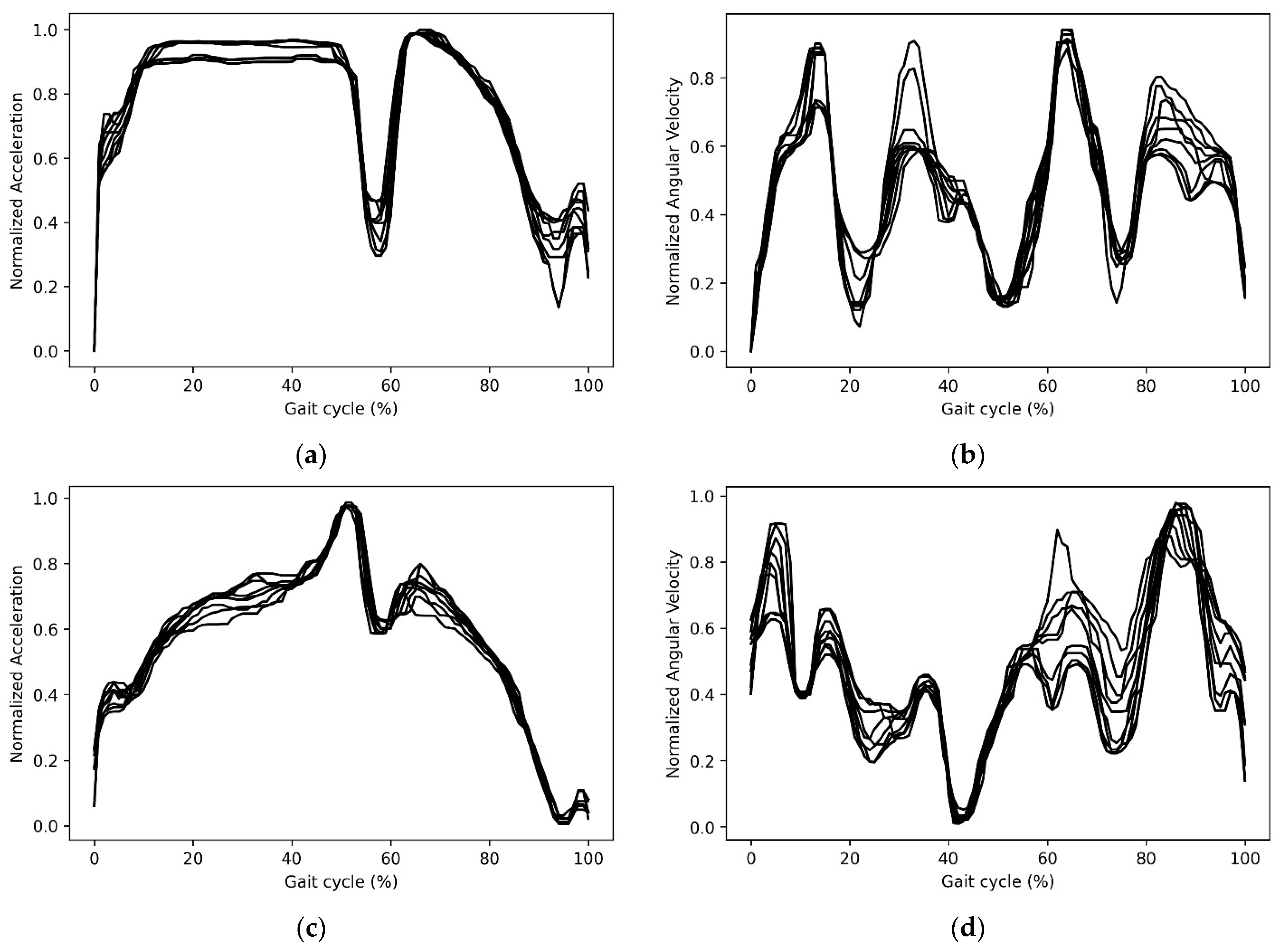
2.1. Gait Dataset
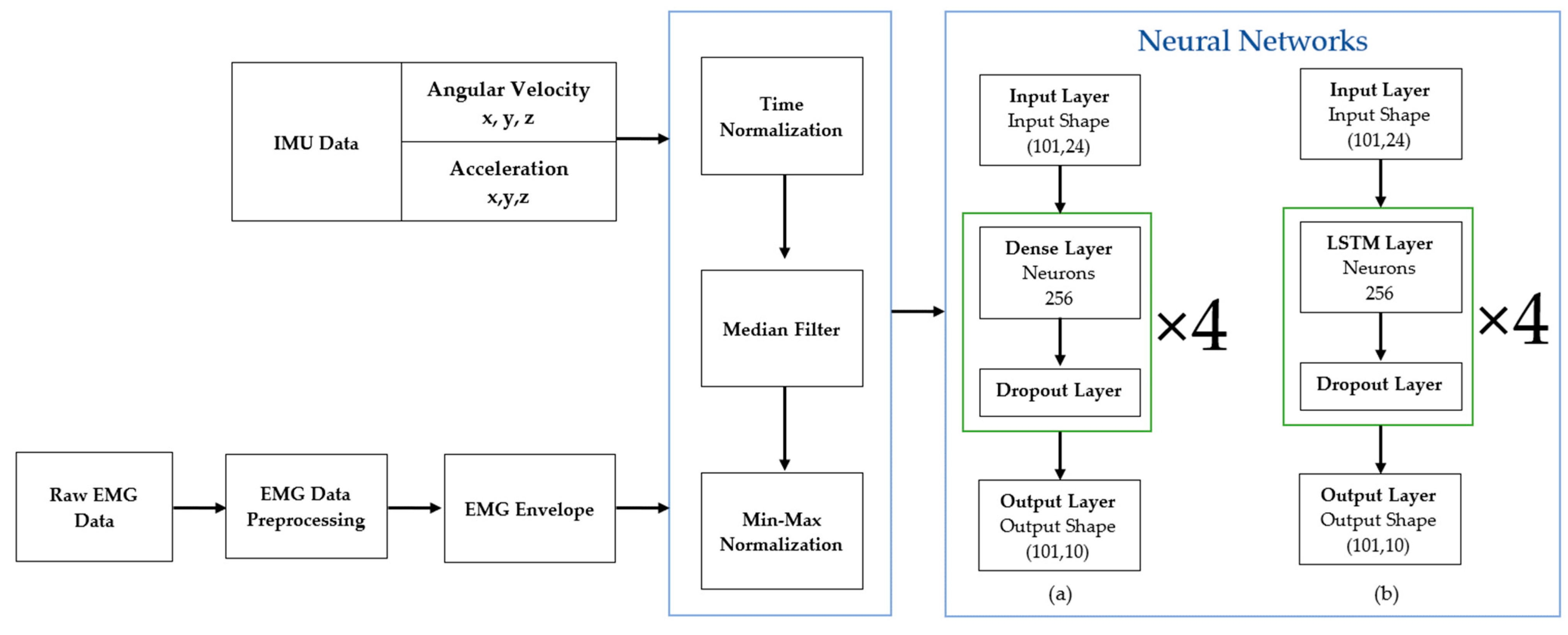
2.2. Data Processing
2.3. Neural Network
2.4. Validation
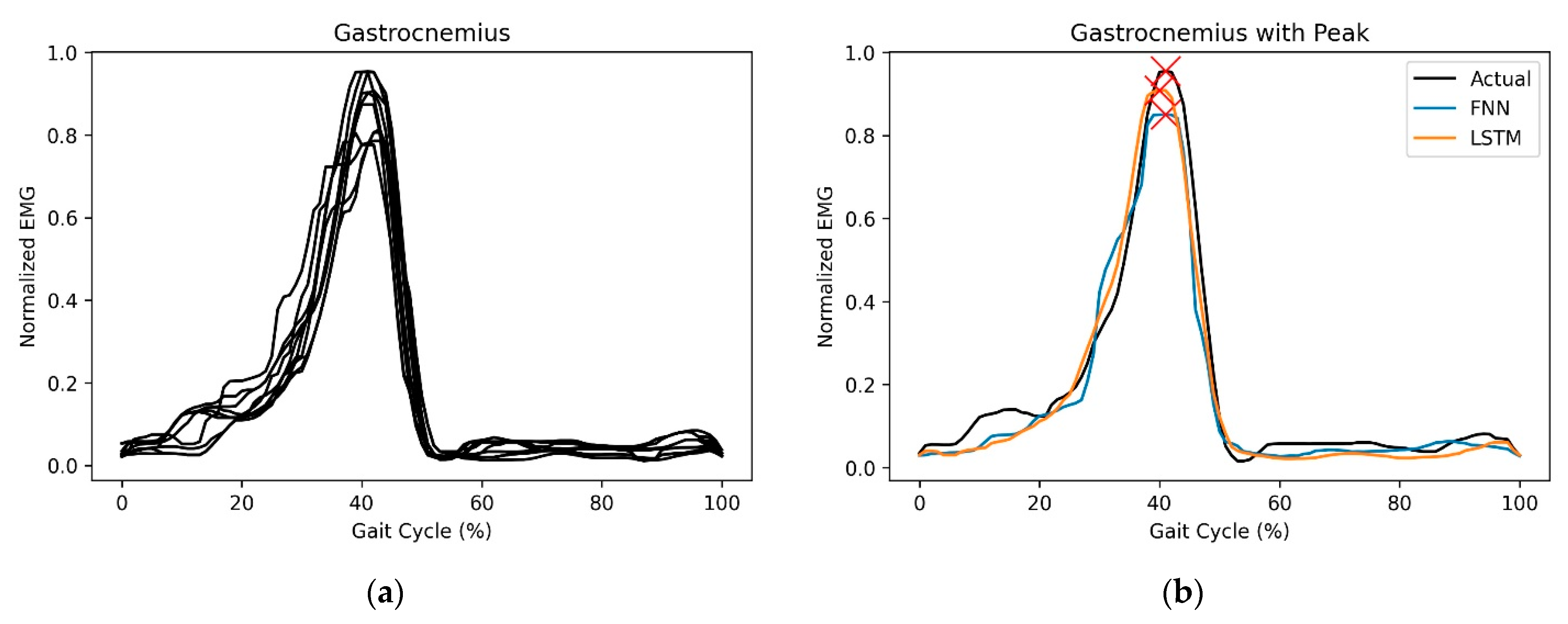
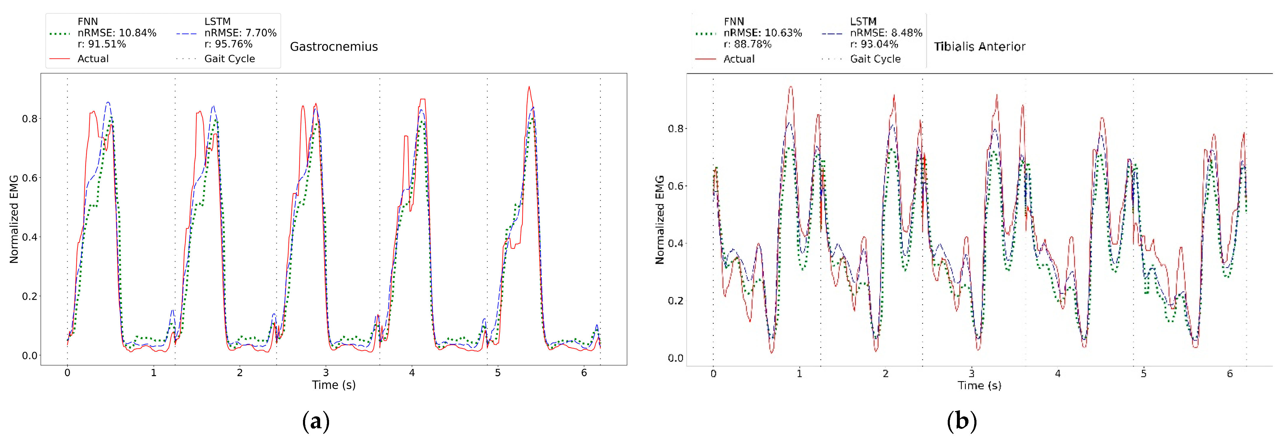
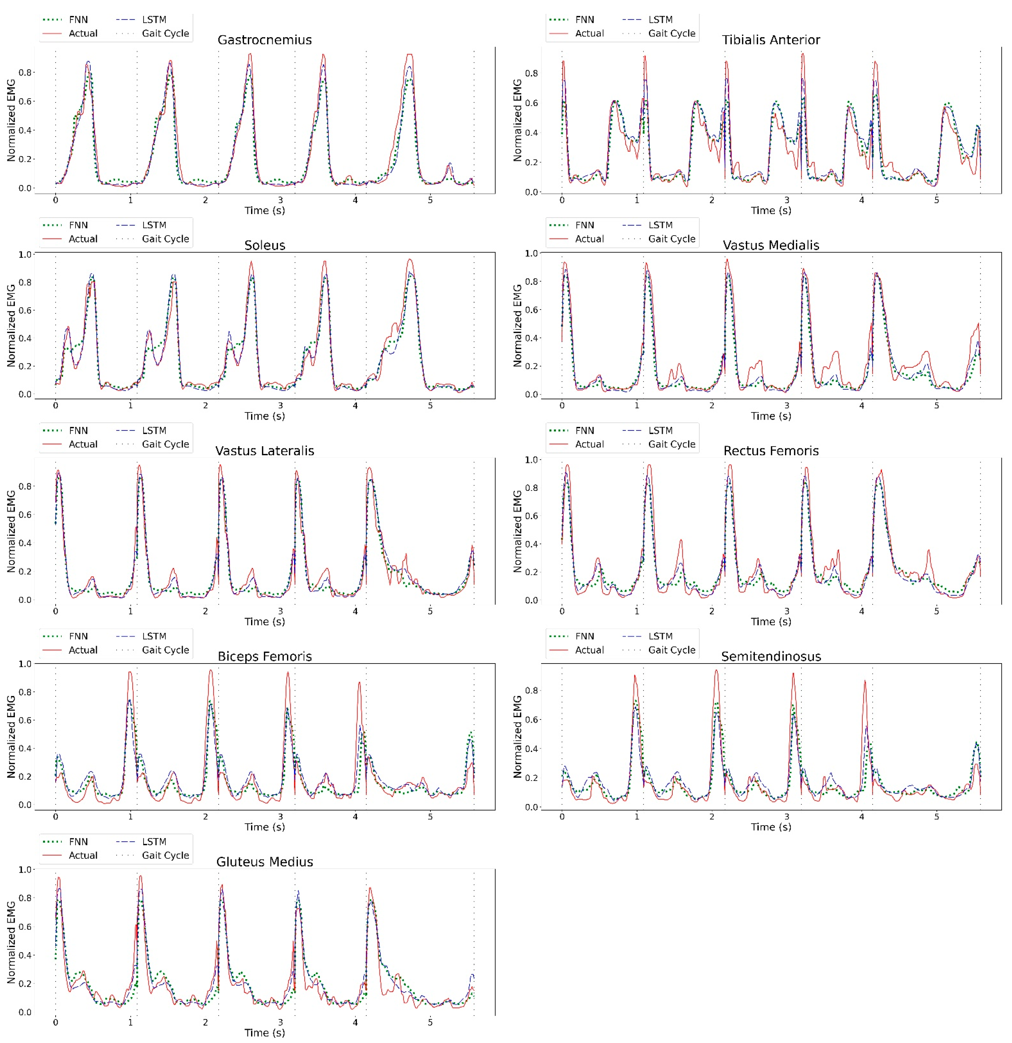
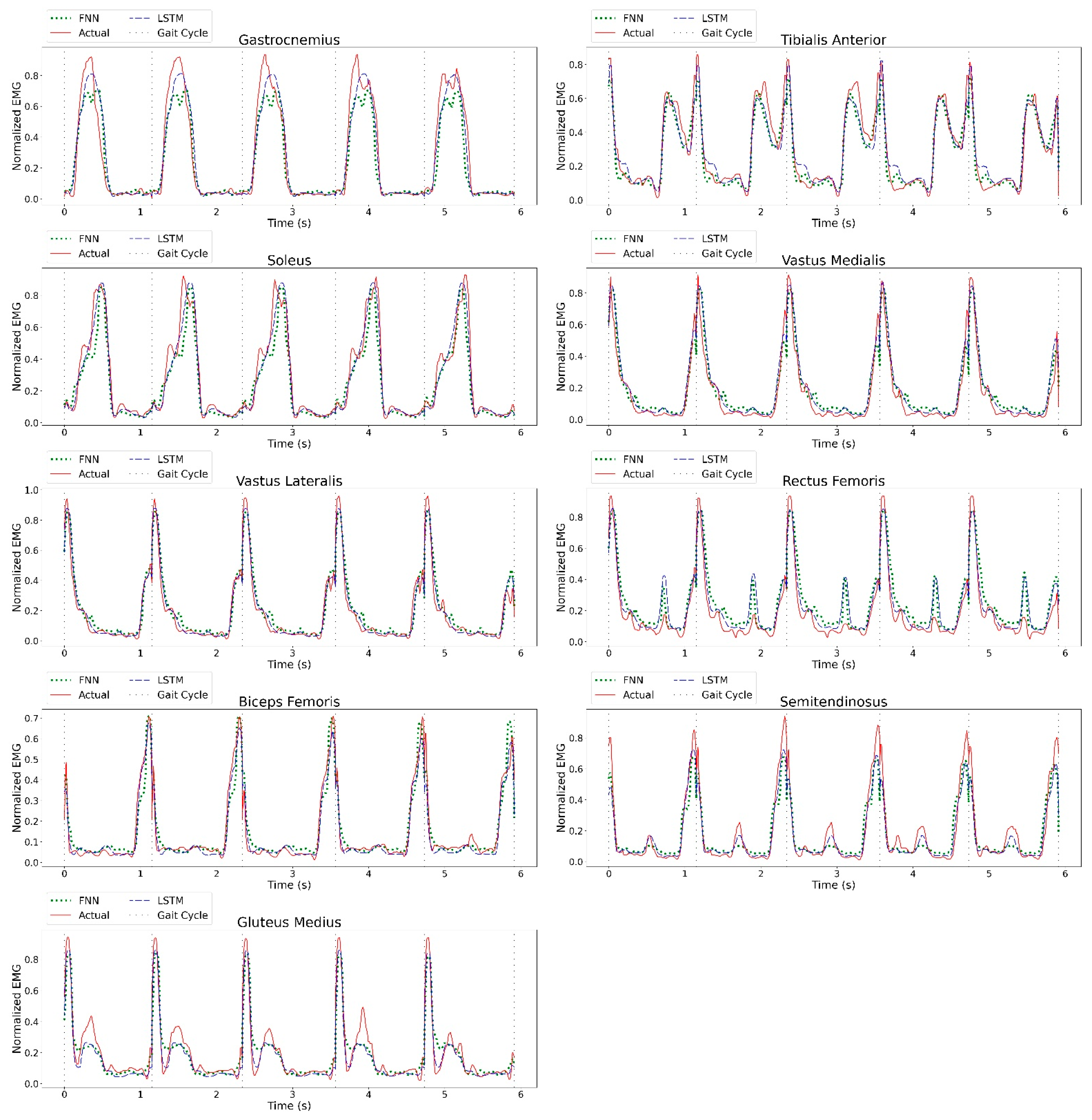
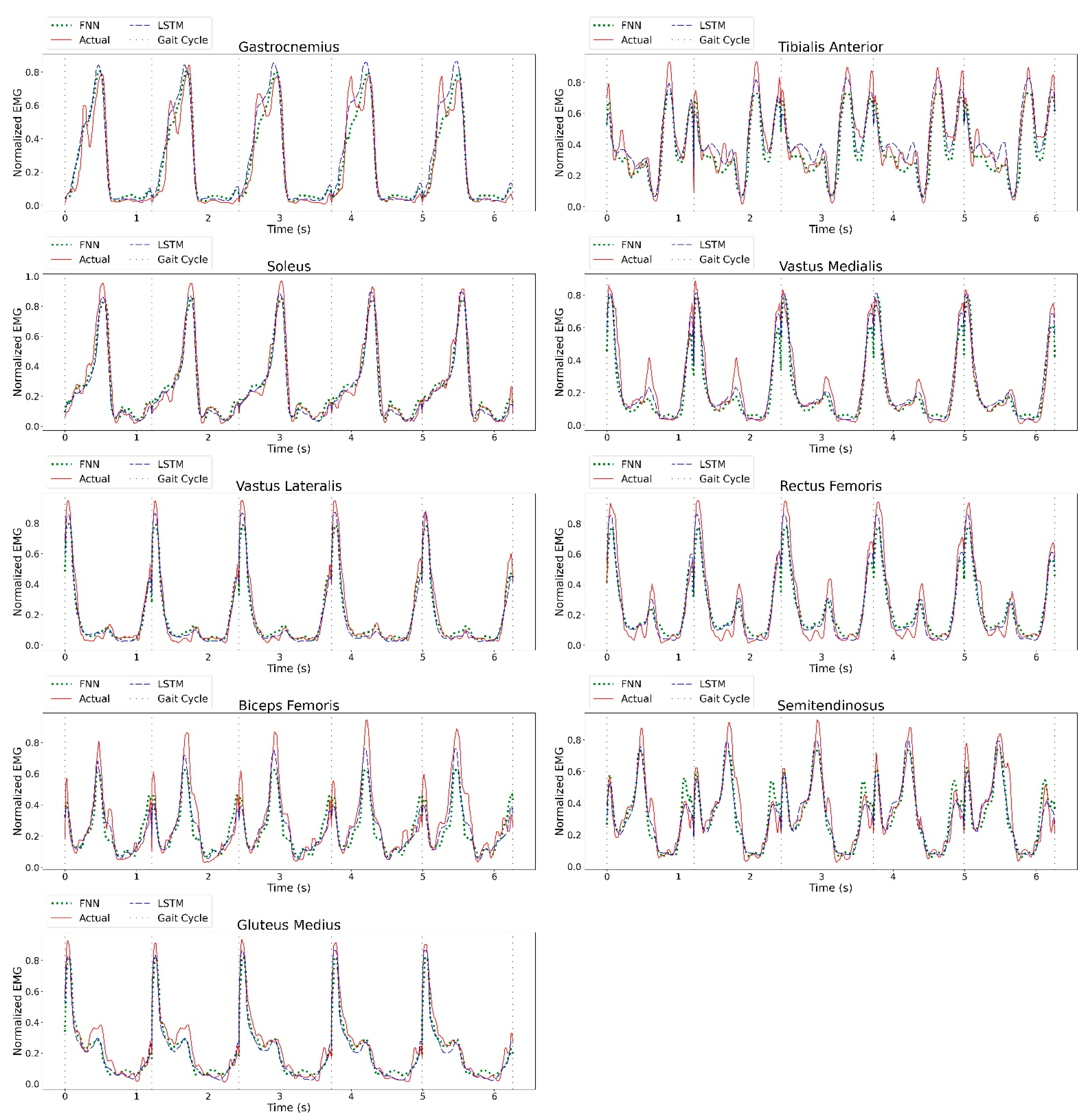
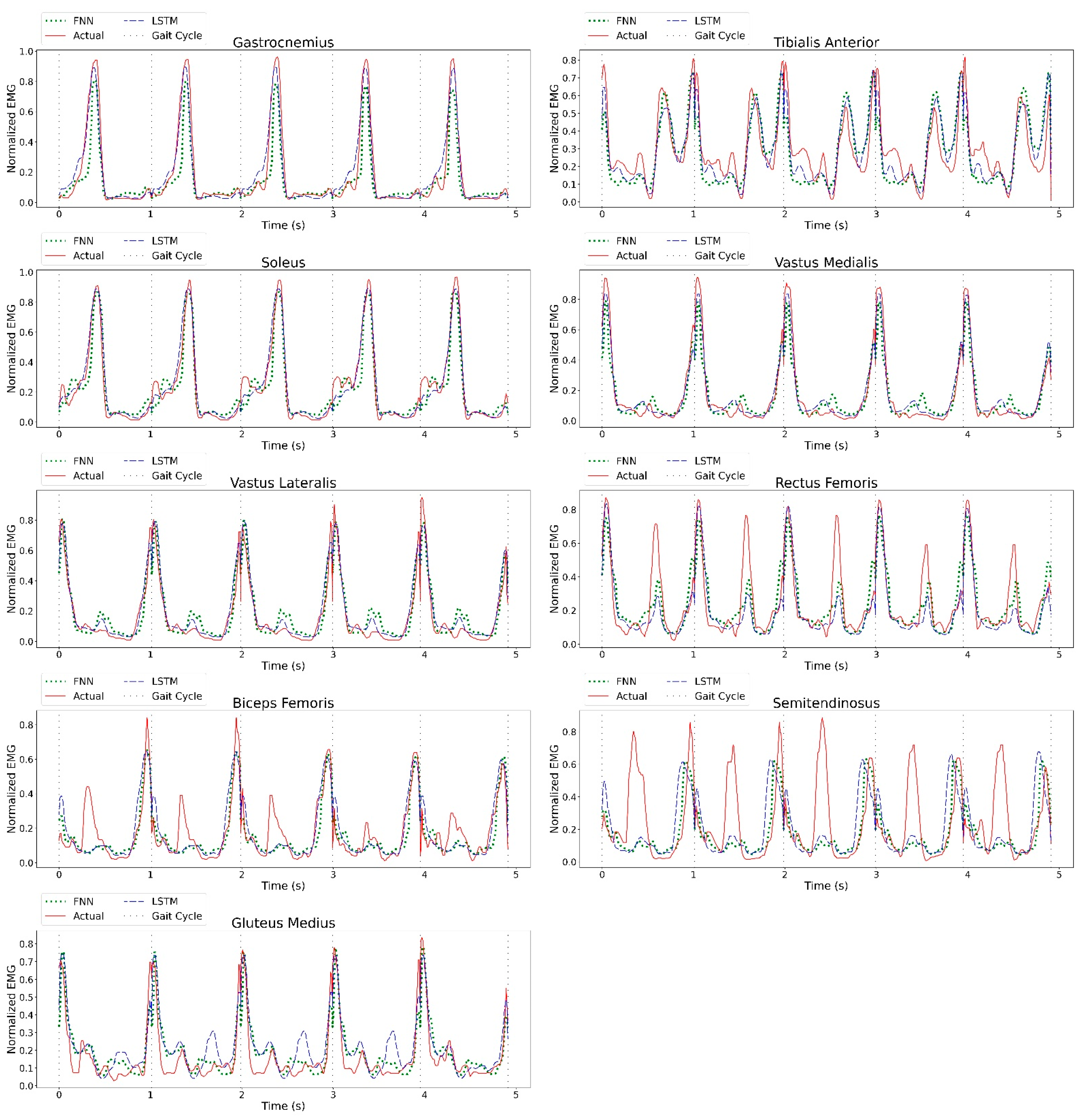
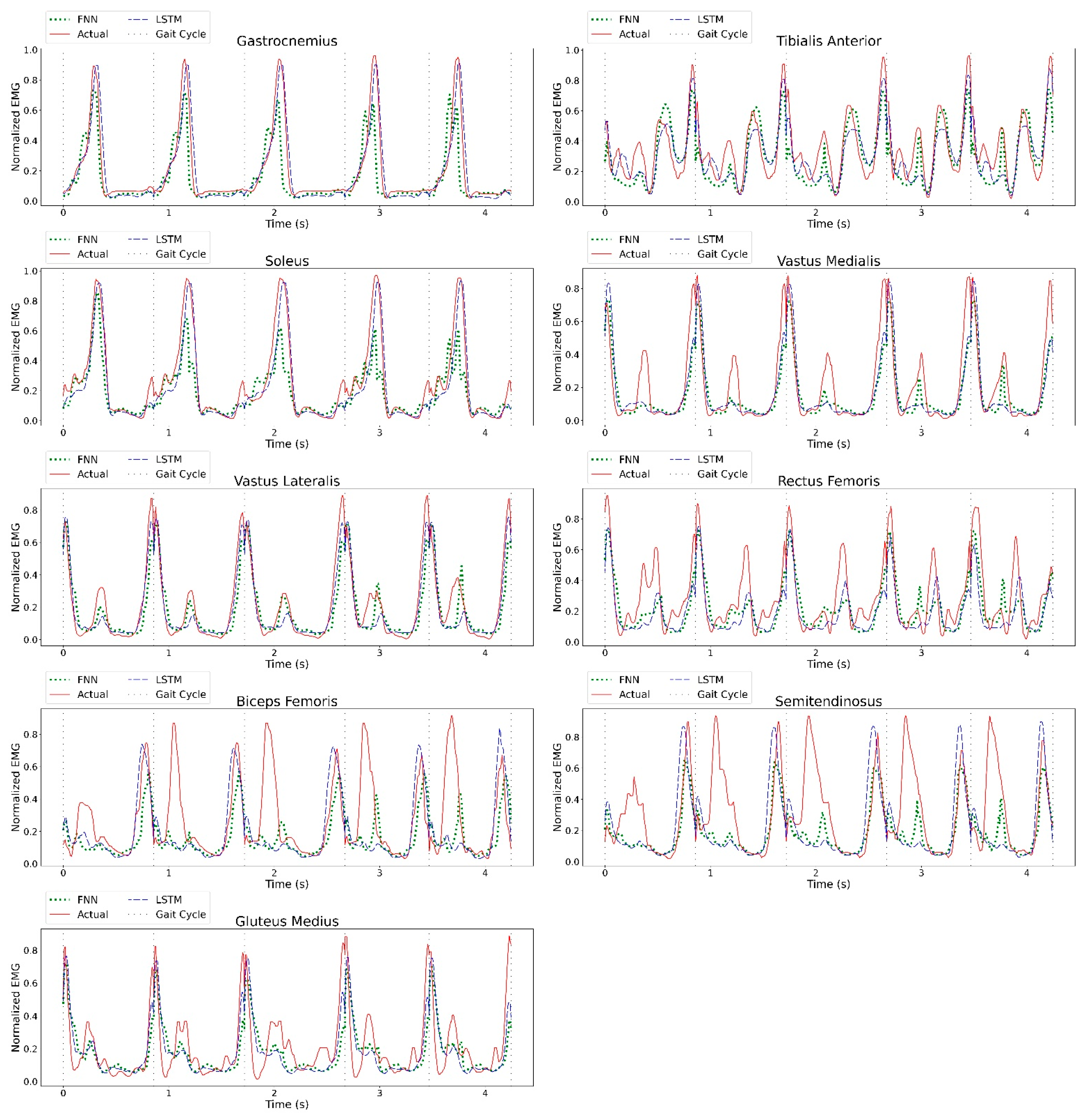
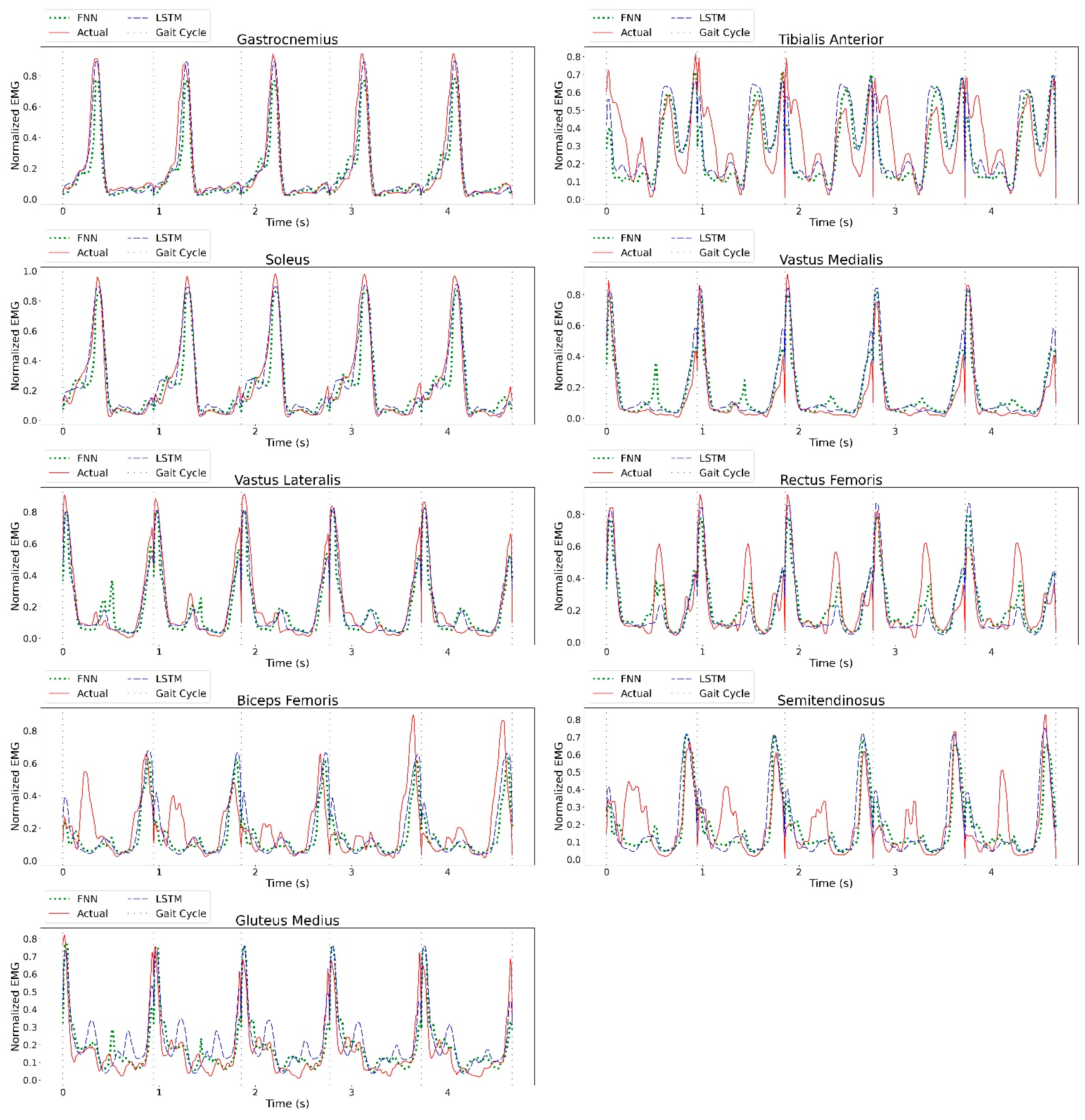
3. Results
4. Discussion
5. Conclusions
Author Contributions
Funding
Institutional Review Board Statement
Informed Consent Statement
Data Availability Statement
Acknowledgments
Conflicts of Interest
Appendix A


Appendix B


References
- Monoli, C.; Fuentez-Pérez, J.F.; Cau, N.; Capodaglio, P.; Galli, M.; Tuhtan, J.A. Land and Underwater Gait Analysis Using Wearable IMU. IEEE Sens. J. 2021, 21, 11192–11202. [Google Scholar] [CrossRef]
- Benson, L.C.; Räisänen, A.M.; Clermont, C.A.; Ferber, R. Is This the Real Life, or Is This Just Laboratory? A Scoping Review of IMU-Based Running Gait Analysis. Sensor 2022, 22, 1722. [Google Scholar] [CrossRef] [PubMed]
- Schicketmueller, A.; Lamprecht, J.; Hofmann, M.; Sailer, M.; Rose, G. Gait Event Detection for Stroke Patients during Robot-Assisted Gait Training. Sensor 2020, 20, 3399. [Google Scholar] [CrossRef] [PubMed]
- Trojaniello, D.; Pelosin, E.; Avanzino, L.; Mirelman, A.; Hausdorff, J.; Della Croce, U. Estimation of step-by-step spatio-temporal parameters of normal and impaired gait using shank-mounted magneto-inertial sensors: Application to elderly, hemiparetic, parkinsonian and choreic gait. J. NeuroEngineering Rehabil. 2014, 11, 152. [Google Scholar] [CrossRef] [PubMed] [Green Version]
- Birch, I.; Nirenberg, M.; Vernon, W.; Birch, M. Forensic Gait Analysis: Principles and Practice; Taylor and Francis: Milton, Canada, 2020. [Google Scholar]
- Kelly, H.D. Forensic Gait Analysis, 1st ed.; CRC Press: Boca Ranton, FL, USA, 2020. [Google Scholar]
- Kwan, R.L.-C.; Zheng, Y.-P.; Cheing, G.L.-Y. The effect of aging on the biomechanical properties of plantar soft tissues. Clin. Biomech. 2010, 25, 601–605. [Google Scholar] [CrossRef]
- Karatsidis, A.; Bellusci, G.; Schepers, H.M.; de Zee, M.; Andersen, M.S.; Veltink, P.H. Estimation of ground reaction forces and moments during gait using only inertial motion capture. Sensor 2017, 17, 75. [Google Scholar] [CrossRef] [Green Version]
- Ancillao, A.; Tedesco, S.; Barton, J.; O’Flynn, B. Indirect Measurement of Ground Reaction Forces and Moments by Means of Wearable Inertial Sensors: A Systematic Review. Sensor 2018, 18, 2564. [Google Scholar] [CrossRef] [Green Version]
- Trinler, U.; Leboeuf, F.; Hollands, K.; Jones, R.; Baker, R. Estimation of muscle activation during different walking speeds with two mathematical approaches compared to surface EMG. Gait Posture 2018, 64, 266–273. [Google Scholar] [CrossRef] [Green Version]
- Zabre-Gonzalez, E.V.; Amieva-Alvarado, D.; Beardsley, S.A. Prediction of EMG Activation Profiles from Gait Kinematics and Kinetics during Multiple Terrains. In Proceedings of the 2021 43rd Annual International Conference of the IEEE Engineering in Medicine & Biology Society (EMBC), Jalisco, Mexico, 1–5 November 2021; pp. 6326–6329. [Google Scholar] [CrossRef]
- Sarshar, M.; Polturi, S.; Schega, L. Gait Phase Estimation by Using LSTM in IMU-Based Gait Analysis-Proof of Concept. Sensor 2021, 21, 5749. [Google Scholar] [CrossRef]
- Lou, Y.; Wang, R.; Mai, J.; Wang, N.; Wang, Q. IMU-Based Gait Phase Recognition for Stroke Survivors. Robotica 2019, 37, 2195–2208. [Google Scholar] [CrossRef]
- Wang, J.; Dai, Y.; Si, X. Analysis and Recognition of Human Lower Limb Motions Based on Electromyography (EMG) Signals. Electronics 2021, 10, 2473. [Google Scholar] [CrossRef]
- Stetter, B.J.; Krafft, F.C.; Ringhof, S.; Stein, T.; Sell, S. A machine learning and wearable sensor based approach to estimate external knee flexion and adduction moments during various locomotion tasks. Front. Bioeng. Biotechnol. 2020, 8, 9. [Google Scholar] [CrossRef] [PubMed]
- Burton, W.S., 2nd; Myers, C.A.; Rullkoetter, P.J. Machine learning for rapid estimation of lower extremity muscle and joint loading during activities of daily living. J. Biomech. 2021, 123, 110439. [Google Scholar] [CrossRef]
- Lu, Y.; Wang, H.; Zhou, B.; Wei, C.; Xu, S. Continuous and simultaneous estimation of lower limb multi-joint angles from sEMG signals based on stacked convolutional and LSTM models. Expert Syst. Appl. 2022, 203, 117340. [Google Scholar] [CrossRef]
- Camargo, J.; Ramanathan, A.; Flanagan, W.; Young, A. A comprehensive, open-source dataset of lower limb biomechanics in multiple conditions of stairs, ramps, and level-ground ambulation and transitions. J. Biomech. 2021, 119, 110320. [Google Scholar] [CrossRef] [PubMed]
- ISEK. Standards for Reporting EMG Data. J. Electromyogr. Kinesiol. 2018, 42, I. [Google Scholar] [CrossRef]
- Pearson, R.K. Chapter 4: Median Filters and Some Extensions. In Nonlinear Digital Filtering with Python: An Introduction, 1st ed.; Gabbouj, M., Ed.; CRC Press: Boca Raton, FL, USA, 2016. [Google Scholar]
- Suzuki, K. Artificial Neural Networks: Methodological Advances and Biomedical Applications; IntechOpen: London, UK, 2011. [Google Scholar]
- Ketkar, N.; Moolayil, J. Deep Learning with Python: Learn Best Practices of Deep Learning Models with Pytorch; Apress L.P.: Berkeley, CA, USA, 2021. [Google Scholar]
- Adams, J.M.; Cerny, K. Observational Gait Analysis: A Visual Guide; SLACK Incorporated: Thorofare, NJ, USA, 2018. [Google Scholar]
- Levine, D.; Richards, J.; Whittle, M.W. Whittle’s Gait Analysis; Elsevier Health Sciences: London, UK, 2012. [Google Scholar]
- Roelker, S.A.; Caruthers, E.J.; Hall, R.K.; Pelz, N.C.; Chaudhari, A.M.W.; Siston, R.A. Effects of Optimization Technique on Simulated Muscle Activations and Forces. J. Appl. Biomech. 2020, 36, 259–278. [Google Scholar] [CrossRef]
- OpenSim. How CMC Works—OpenSim Documentation—Global Site. Available online: https://simtk-confluence.stanford.edu:8443/display/OpenSim/How+CMC+Works (accessed on 29 October 2022).
- den Otter, A.R.; Geurts, A.C.H.; Mulder, T.; Duysens, J. Speed related changes in muscle activity from normal to very slow walking speeds. Gait Posture 2004, 19, 270–278. [Google Scholar] [CrossRef] [Green Version]
- Escalona, M.J.; Bourbonnais, D.; Goyette, M.; Le Flem, D.; Duclos, C.; Gagnon, D.H. Effects of Varying Overground Walking Speeds on Lower-Extremity Muscle Synergies in Healthy Individuals. Mot. Control 2021, 25, 234–251. [Google Scholar] [CrossRef]
- Nene, A.; Byrne, C.; Hermens, H. Is rectus femoris really a part of quadriceps?: Assessment of rectus femoris function during gait in able-bodied adults. Gait Posture 2004, 20, 1–13. [Google Scholar] [CrossRef]
- Barr, K.M.; Miller, A.L.; Chapin, K.B. Surface electromyography does not accurately reflect rectus femoris activity during gait: Impact of speed and crouch on vasti-to-rectus crosstalk. Gait Posture 2010, 32, 363–368. [Google Scholar] [CrossRef]
- Mesin, L. Crosstalk in surface electromyogram: Literature review and some insights. (in eng). Phys. Eng. Sci. Med. 2020, 43, 481–492. [Google Scholar] [CrossRef]
- Riley, P.O.; DellaCroce, U.; Kerrigan, D.C. Effect of age on lower extremity joint moment contributions to gait speed. (in eng). Gait Posture 2001, 14, 264–270. [Google Scholar] [CrossRef] [PubMed]
- Silder, A.; Heiderscheit, B.; Thelen, D.G. Active and passive contributions to joint kinetics during walking in older adults. (in eng). J. Biomech. 2008, 41, 1520–1527. [Google Scholar] [CrossRef] [PubMed] [Green Version]
- Van Criekinge, T.; Saeys, W.; Hallemans, A.; Van de Walle, P.; Vereeck, L.; De Hertogh, W.; Truijen, S. Age-related differences in muscle activity patterns during walking in healthy individuals. (in eng). J. Electromyogr. Kinesiol. 2018, 41, 124–131. [Google Scholar] [CrossRef] [PubMed]
- Assaiante, C. Development of locomotor balance control in healthy children. Neurosci. Biobehav. Rev. 1998, 22, 527–532. [Google Scholar] [CrossRef] [PubMed]
- Jain, E.; Anthony, L.; Aloba, A.; Castonguay, A.; Cuba, I.; Shaw, A. Is the motion of a child perceivably different from the motion of an adult? ACM Trans. Appl. Percept. (TAP) 2016, 13, 22. [Google Scholar] [CrossRef]
- Cohen, R.; Mitchell, C.; Dotan, R.; Gabriel, D.; Klentrou, P.; Falk, B. Do neuromuscular adaptations occur in endurance-trained boys and men? Appl. Physiol. Nutr. Metab. 2010, 35, 471–479. [Google Scholar] [CrossRef]
- Bao, T.; Zaidi, S.A.R.; Xie, S.; Yang, P.; Zhang, Z.-Q. A CNN-LSTM hybrid model for wrist kinematics estimation using surface electromyography. IEEE Trans. Instrum. Meas. 2020, 70, 1–9. [Google Scholar] [CrossRef]


| Group | Number of Trials | Number of Gaits |
|---|---|---|
| Training | 440 | 4318 |
| Validation | 80 | 818 |
| Testing | 30 | 304 |
| Unseen subject | 30 | 303 |
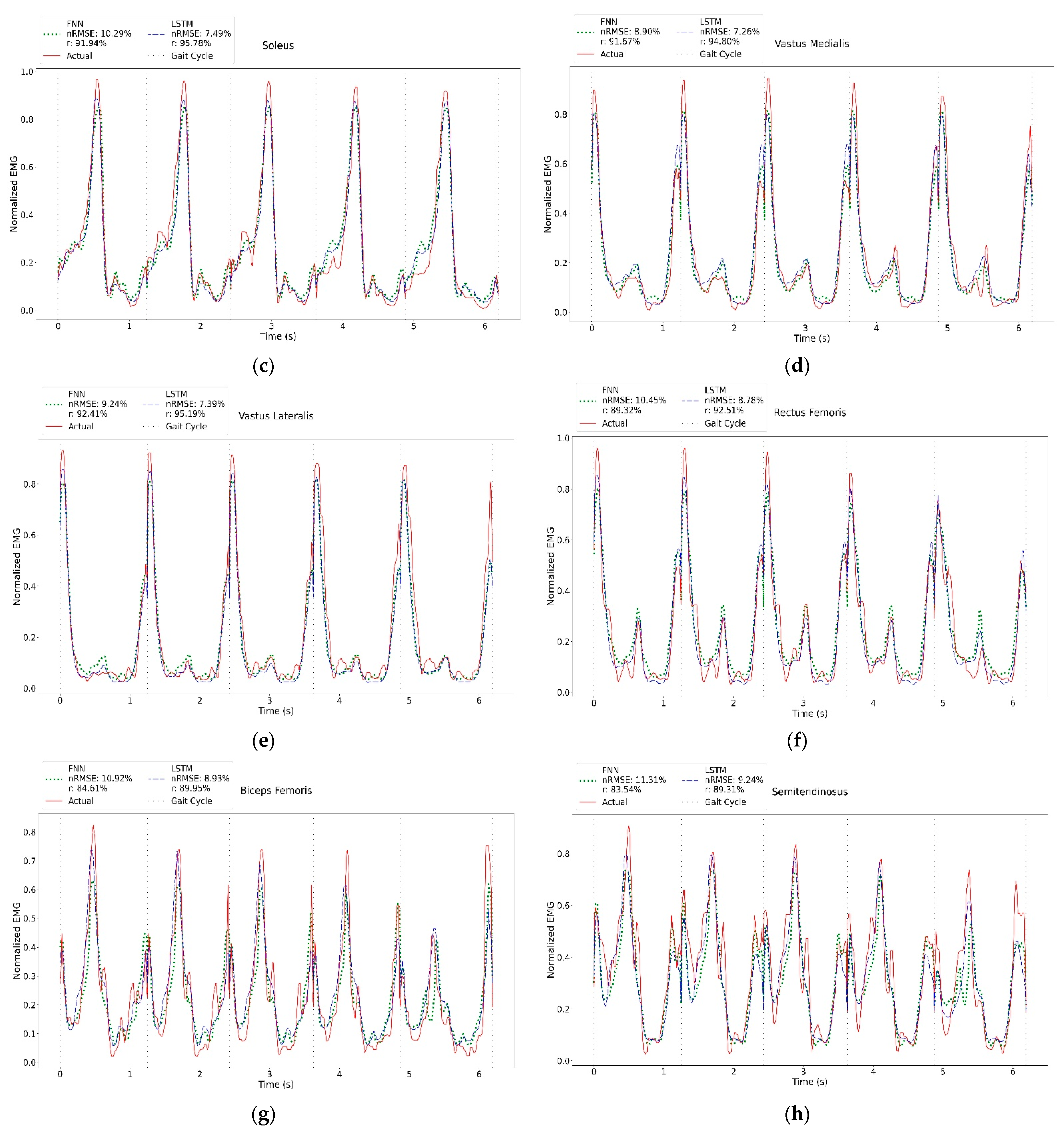
| Muscles | FNN | LSTM | ||||||
|---|---|---|---|---|---|---|---|---|
| nRMSE (%) | r (%) | ∆Tp (%) | ∆Ep (%) | nRMSE (%) | r (%) | ∆Tp (%) | ∆Ep (%) | |
| Gastrocnemius | 10.84 | 91.51 | 2.59 ± 2.91 | 12.96 ± 7.08 | 7.70 | 95.76 | 2.40 ± 2.60 | 9.21 ± 5.88 |
| Tibialis Anterior | 10.63 | 88.78 | 0.71 ± 2.14 | 17.47 ± 10.16 | 8.48 | 93.04 | 0.72 ± 2.16 | 13.73 ± 10.58 |
| Soleus | 10.29 | 91.94 | 2.13 ± 1.79 | 9.08 ± 6.61 | 7.49 | 95.78 | 2.11 ± 1.81 | 10.54 ± 5.58 |
| Vastus Medialis | 8.90 | 91.67 | 0.93 ± 0.83 | 12.30 ± 10.56 | 7.26 | 94.80 | 0.86 ± 0.88 | 9.60 ± 10.23 |
| Vastus Lateralis | 9.24 | 92.41 | 0.94 ± 0.80 | 9.18 ± 7.22 | 7.39 | 95.19 | 0.87 ± 0.84 | 9.02 ± 6.16 |
| Rectus Femoris | 10.45 | 89.32 | 1.60 ± 1.65 | 12.88 ± 9.37 | 8.78 | 92.51 | 1.56 ± 1.74 | 12.37 ± 15.29 |
| Biceps Femoris | 10.92 | 84.61 | 1.82 ± 1.59 | 22.33 ± 15.07 | 8.93 | 89.95 | 1.71 ± 1.43 | 20.35 ± 14.52 |
| Semitendinosus | 11.31 | 83.54 | 2.43 ± 2.57 | 20.95 ± 14.87 | 9.24 | 89.31 | 2.31 ± 2.58 | 18.16 ± 14.30 |
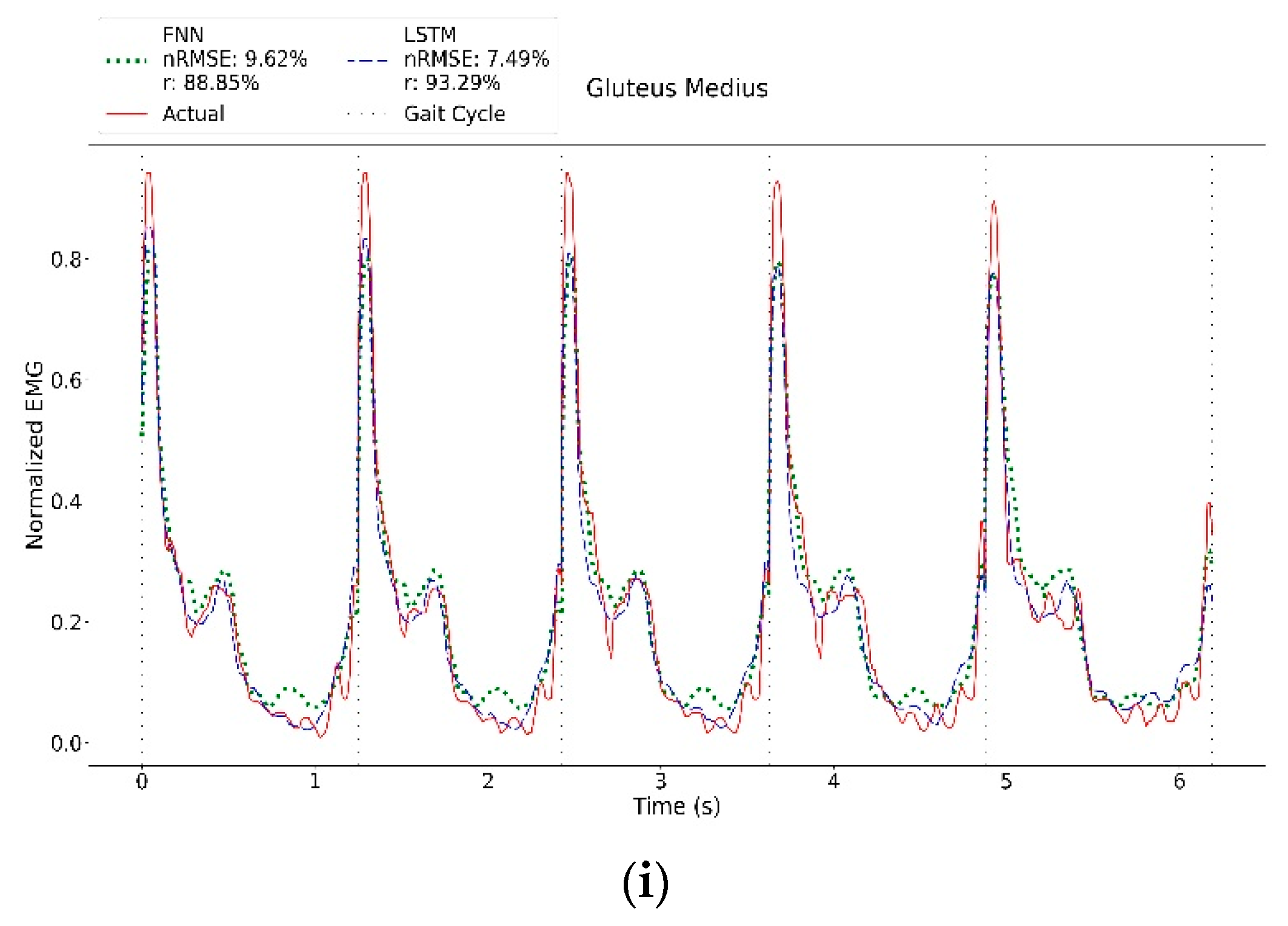
| Gluteus Medius | 9.62 | 88.85 | 1.31 ± 2.29 | 18.11 ± 52.10 | 7.49 | 93.29 | 1.20 ± 2.31 | 15.48 ± 47.72 |
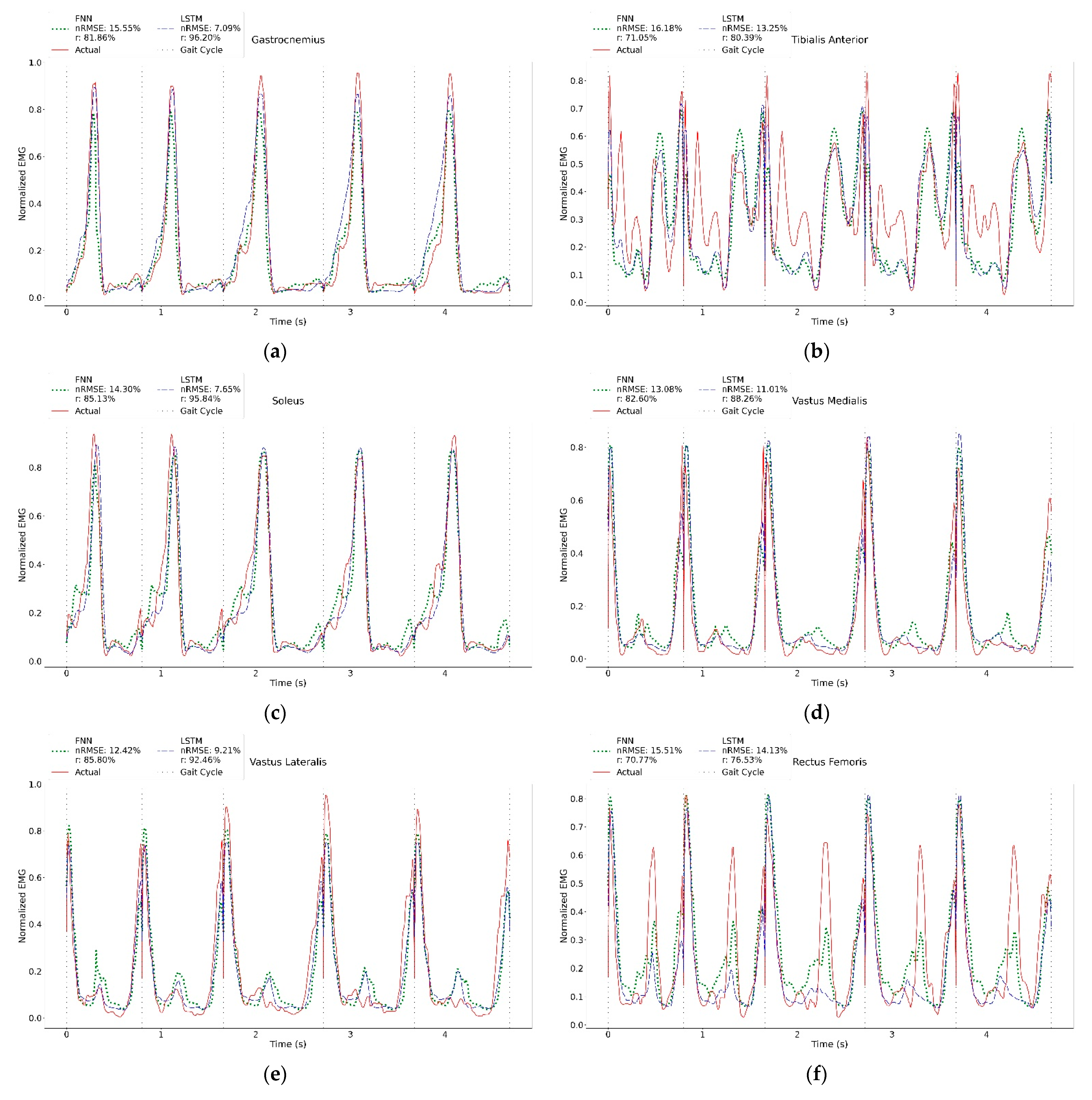
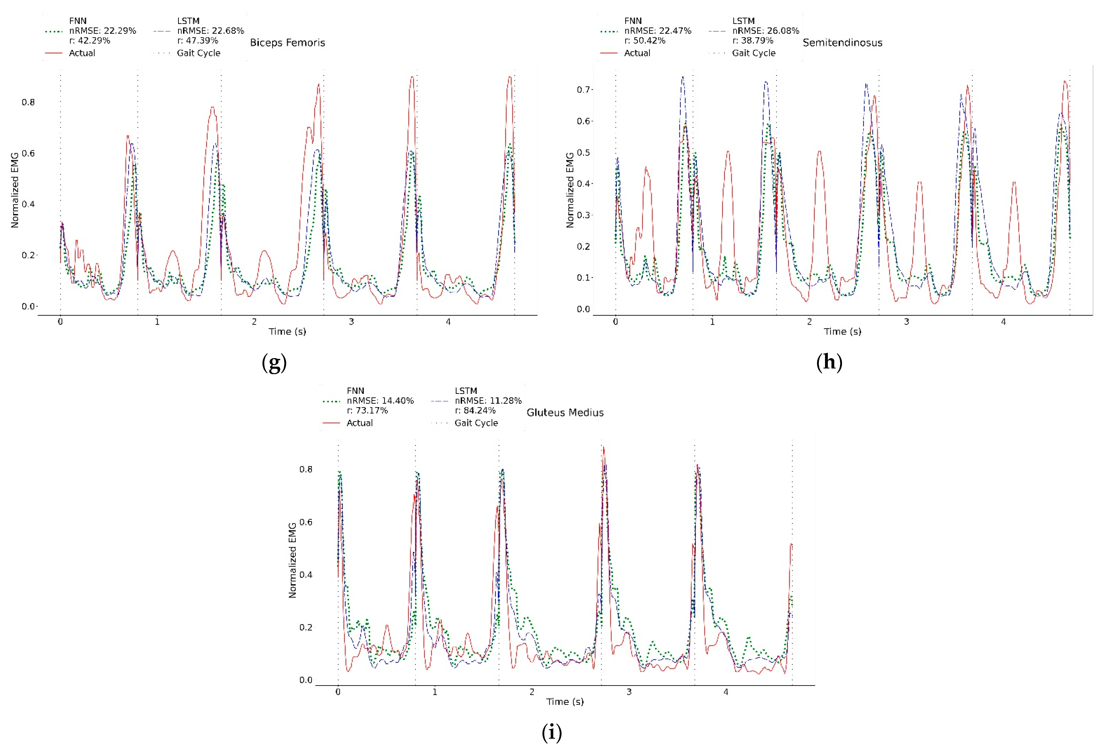
| Muscle | FNN | LSTM | Other Studies | |||||||
|---|---|---|---|---|---|---|---|---|---|---|
| nRMSE (%) | r (%) | ∆Tp (%) | ∆Ep (%) | nRMSE (%) | r (%) | ∆Tp (%) | ∆Ep (%) | nRMSE (%) [11] | r (%) [10] | |
| Gastrocnemius | 15.55 | 81.86 | 1.57 ± 1.80 | 19.36 ± 9.77 | 7.09 | 96.20 | 1.47 ± 1.08 | 10.84 ± 12.73 | 11.0 | 93 |
| Tibialis Anterior | 16.18 | 71.05 | 3.89 ± 10.20 | 31.41 ± 32.21 | 13.25 | 80.39 | 1.75 ± 5.50 | 18.30 ± 43.19 | 12.6 | 66 |
| Soleus | 14.30 | 85.13 | 1.91 ± 1.65 | 18.32 ± 9.45 | 7.65 | 95.84 | 1.90 ± 1.42 | 8.24 ± 2.81 | - | 96 |
| Vastus Medialis | 13.08 | 82.60 | 0.78 ± 0.62 | 12.84 ± 22.10 | 11.01 | 88.26 | 1.44 ± 0.65 | 14.34 ± 24.80 | - | 60 |
| Vastus Lateralis | 12.42 | 85.80 | 0.91 ± 0.82 | 12.13 ± 24.22 | 9.21 | 92.46 | 1.27 ± 0.80 | 17.53 ± 23.29 | - | 61 |
| Rectus Femoris | 15.51 | 70.77 | 1.49 ± 3.21 | 20.20 ± 35.08 | 14.13 | 76.53 | 1.70 ± 3.52 | 21.79 ± 39.68 | - | 54 |
| Biceps Femoris | 22.29 | 42.29 | 4.17 ± 2.91 | 24.00 ± 19.82 | 22.68 | 47.39 | 2.43 ± 1.99 | 36.44 ± 33.66 | - | - |
| Semitendinosus | 22.47 | 50.42 | 2.62 ± 2.09 | 23.88 ± 17.96 | 26.08 | 38.79 | 4.52 ± 2.39 | 24.73 ± 26.10 | - | 54 |
| Gluteus Medius | 14.40 | 73.17 | 0.82 ± 2.59 | 11.64 ± 12.84 | 11.28 | 84.24 | 1.70 ± 2.14 | 10.59 ± 13.91 | - | - |
Disclaimer/Publisher’s Note: The statements, opinions and data contained in all publications are solely those of the individual author(s) and contributor(s) and not of MDPI and/or the editor(s). MDPI and/or the editor(s) disclaim responsibility for any injury to people or property resulting from any ideas, methods, instructions or products referred to in the content. |
© 2023 by the authors. Licensee MDPI, Basel, Switzerland. This article is an open access article distributed under the terms and conditions of the Creative Commons Attribution (CC BY) license (https://creativecommons.org/licenses/by/4.0/).
Share and Cite
Khant, M.; Gouwanda, D.; Gopalai, A.A.; Lim, K.H.; Foong, C.C. Estimation of Lower Extremity Muscle Activity in Gait Using the Wearable Inertial Measurement Units and Neural Network. Sensors 2023, 23, 556. https://doi.org/10.3390/s23010556
Khant M, Gouwanda D, Gopalai AA, Lim KH, Foong CC. Estimation of Lower Extremity Muscle Activity in Gait Using the Wearable Inertial Measurement Units and Neural Network. Sensors. 2023; 23(1):556. https://doi.org/10.3390/s23010556
Chicago/Turabian StyleKhant, Min, Darwin Gouwanda, Alpha A. Gopalai, King Hann Lim, and Chee Choong Foong. 2023. "Estimation of Lower Extremity Muscle Activity in Gait Using the Wearable Inertial Measurement Units and Neural Network" Sensors 23, no. 1: 556. https://doi.org/10.3390/s23010556