
Skeleton Graph-Neural-Network-Based Human Action Recognition: A Survey


Abstract
:1. Introduction
- The traditional method is handcrafted descriptors, such as principle components analysis (PCA) based on 3D position differences of joints [11], selecting joint pairs by top-K Relative Variance of Joint Relative Distance [12]. These descriptors are interpretable; however, they are limited as they tend to extract shallow and simple features and normally fail to find significant deep features.
- The other idea is redefining the problem a deep learning problem in Euclidean space, such as serializing the graph nodes into a sequence and then adopting the well-known Convolutional Neural Networks (CNN), Recurrent Neural Networks (RNN) etc. In this way, deep features are extracted mechanically but without paying attention to the intrinsic spatial and temporal relations between graph joints, e.g., the serialization of joints ignores their natural structures in skeletons.
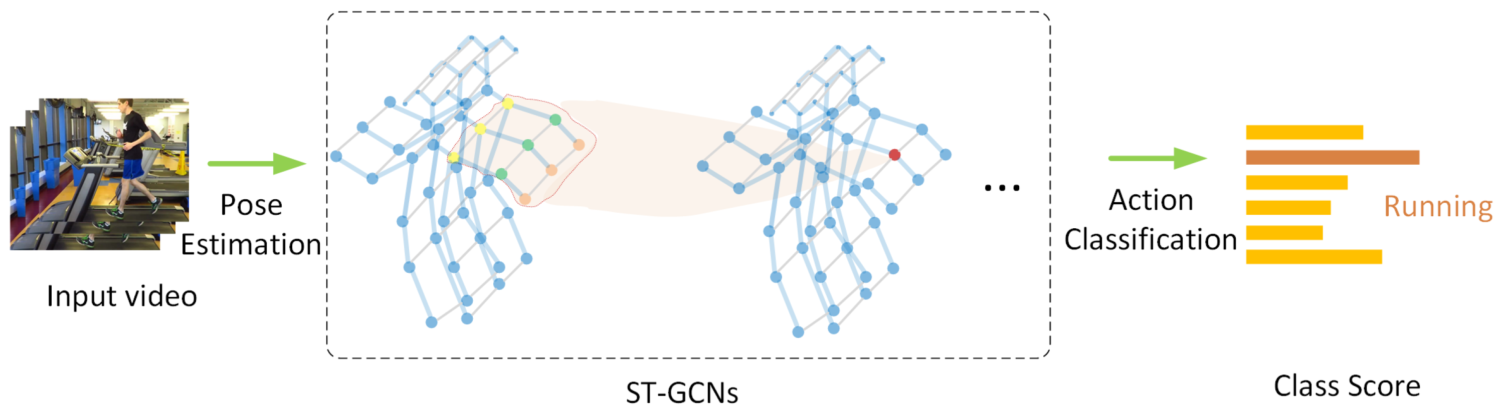
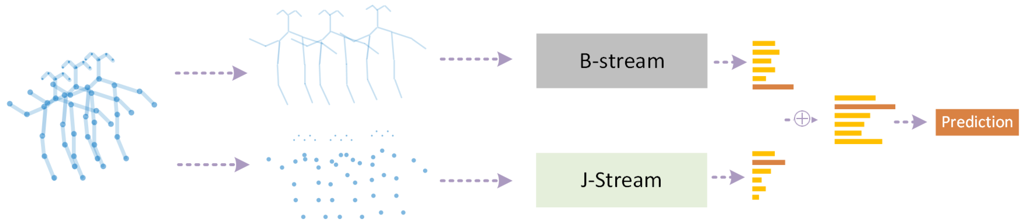
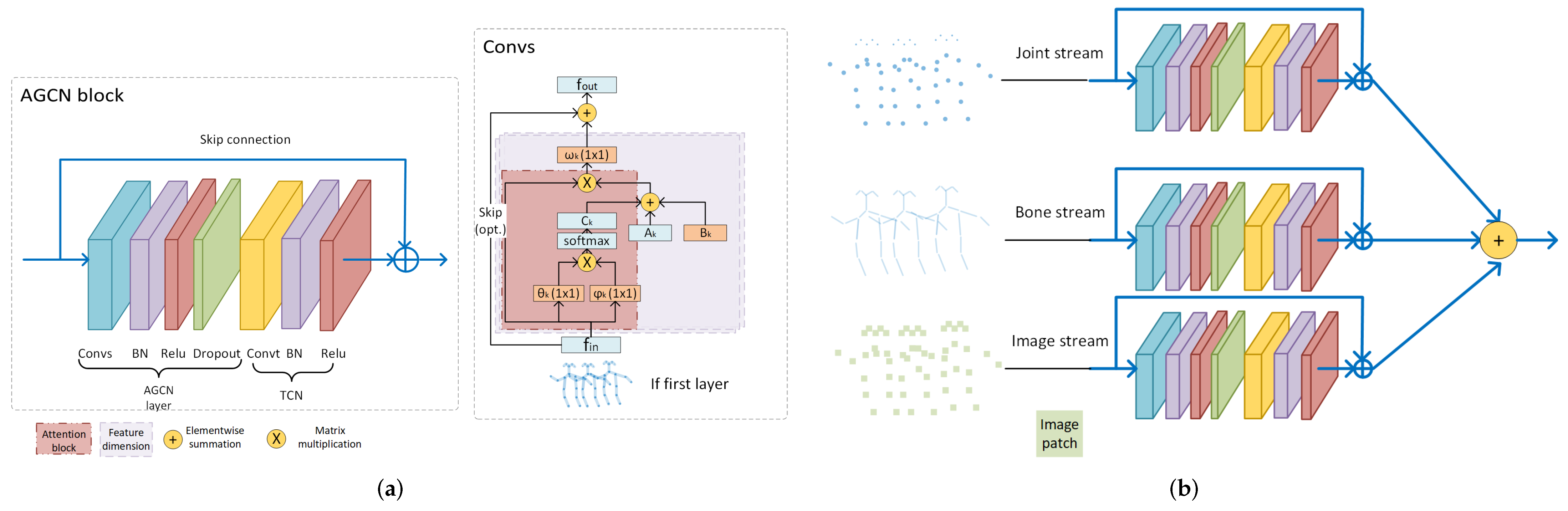
- Recently, Graph Neural Networks (GNNs), especially graph convolution networks (GCNs), have come into spotlight, and were imported into skeleton graphs. The earliest milestone is ST-GCN [13] (Figure 1). Thereafter, multiple works based on ST-GCN were proposed. Among them, 2s-AGCN [14] (Figure 2) is another typical work, which adopted an attention mechanism. As GNNs are professional in discovering the intrinsic relations between joints, GNN HAR methods have achieved a new state-of-the-art (SOTA).
- 1.
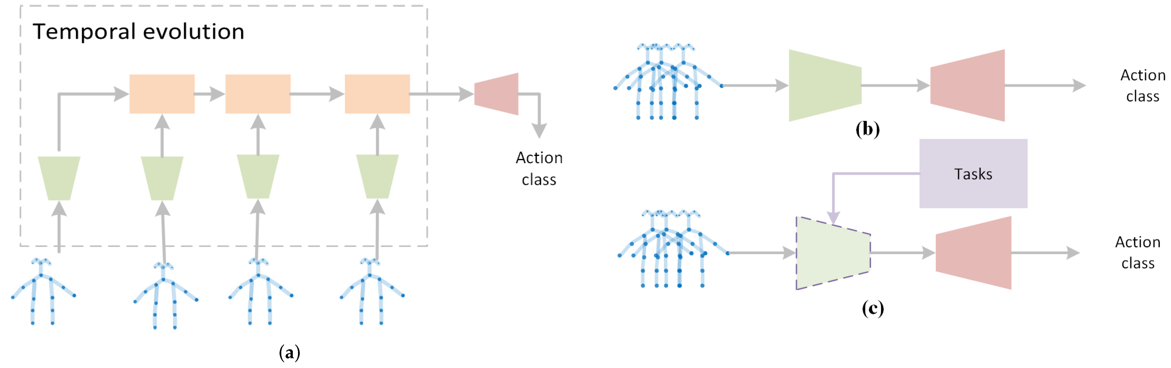
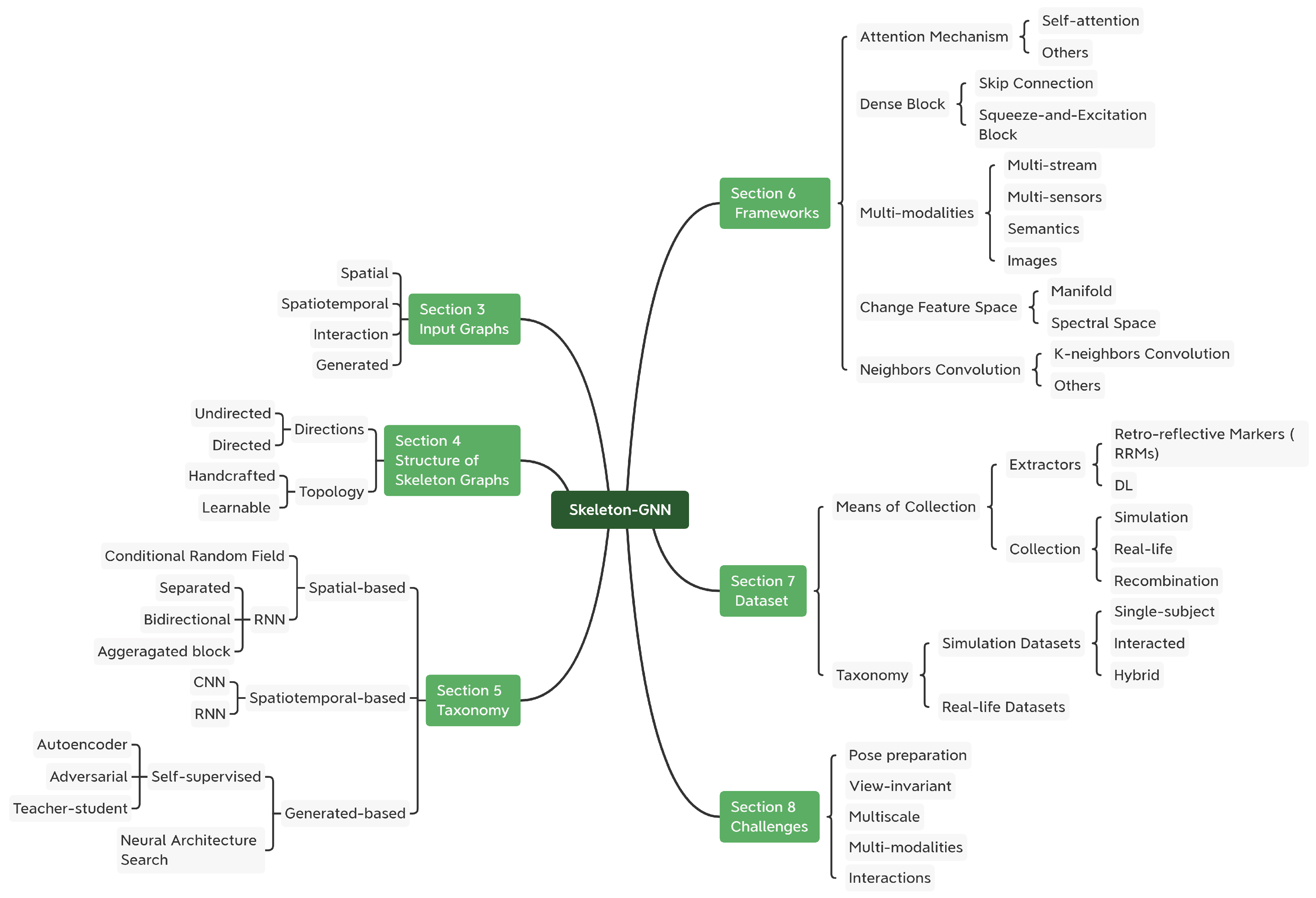
- New taxonomy: We propose a new taxonomy for previous methods, which relate to GNNs and skeleton graphs. They are grouped into spatial-based approaches, spatiotemporal-based approaches and generated approaches. Figure 3 illustrates the idea. Their common frameworks are also summarized.
- 2.
- Comprehensive review: Apart from analyzing methods, we also review the categories of skeleton graphs in applications and the construction of them.
- 3.
- Abundant resources: To give a complete summary for the skeleton-GNN-based HAR, we collected commonly used datasets and published codes. The details of each collected dataset and method are summarized in Table A1 and Table A3, respectively, in Appendix A and Appendix B.
- 4.
- Future directions: Further directions are presented and discussed after having a look at the challenges in this field, with the hope of offering some inspiration for the benefit of other researchers.
2. Previous Works
2.1. GNNs
2.2. HAR Surveys
- 1.
- 2.
- 3.
- 4.
- Papers on methodologies, where [32] dived into GCN-based approaches [23,33,34,35,36,37] collected DL-based methods, and [38] collected both handcrafted-based methods and learning-based methods. Specifically [36,37] only summarized CNN-based approaches, while others analyzed all kinds of DL approaches.
- 5.
- Papers on evaluation, such as [39], gathered the evaluation metrics applied on HAR tasks.
- 6.
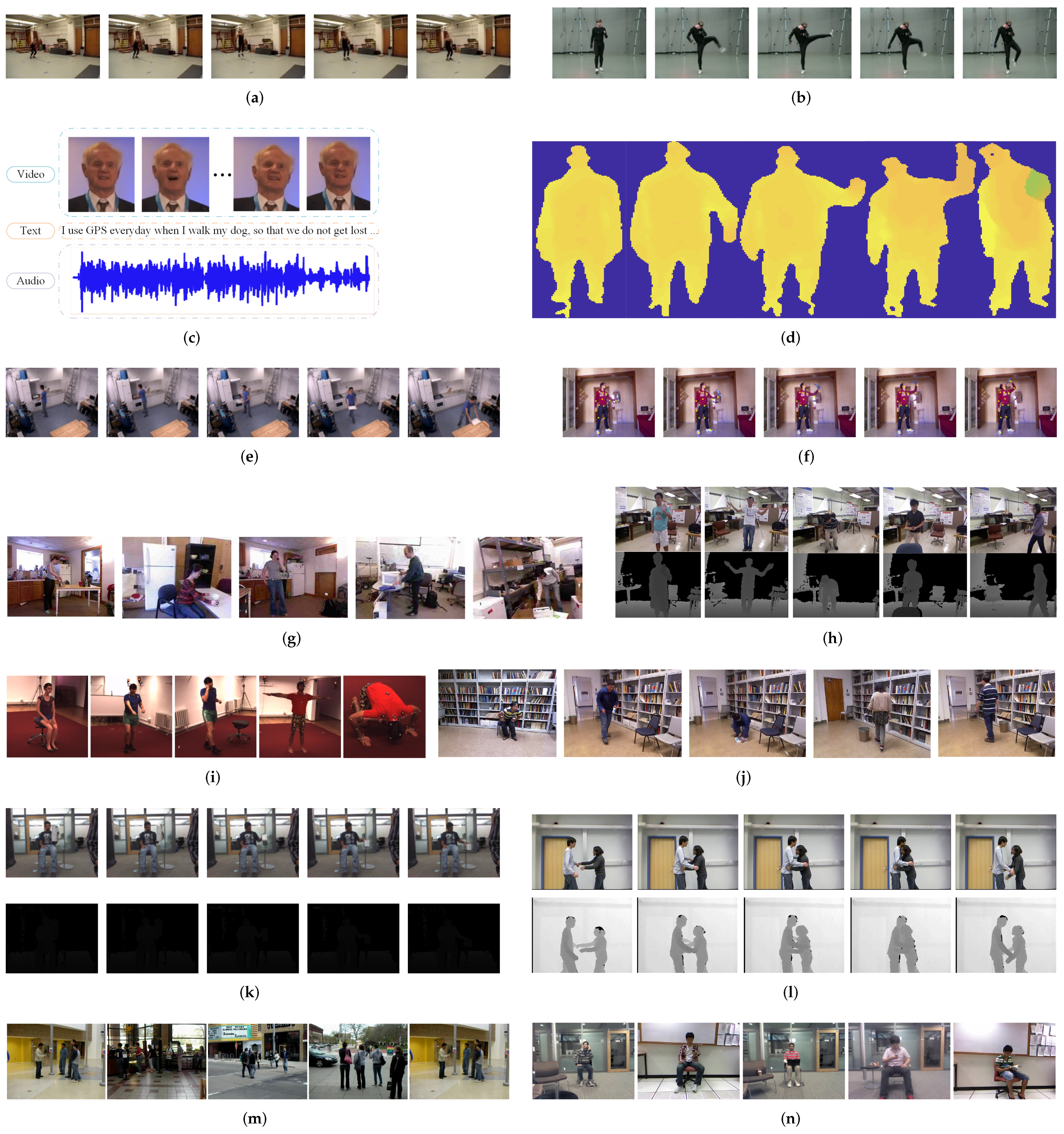
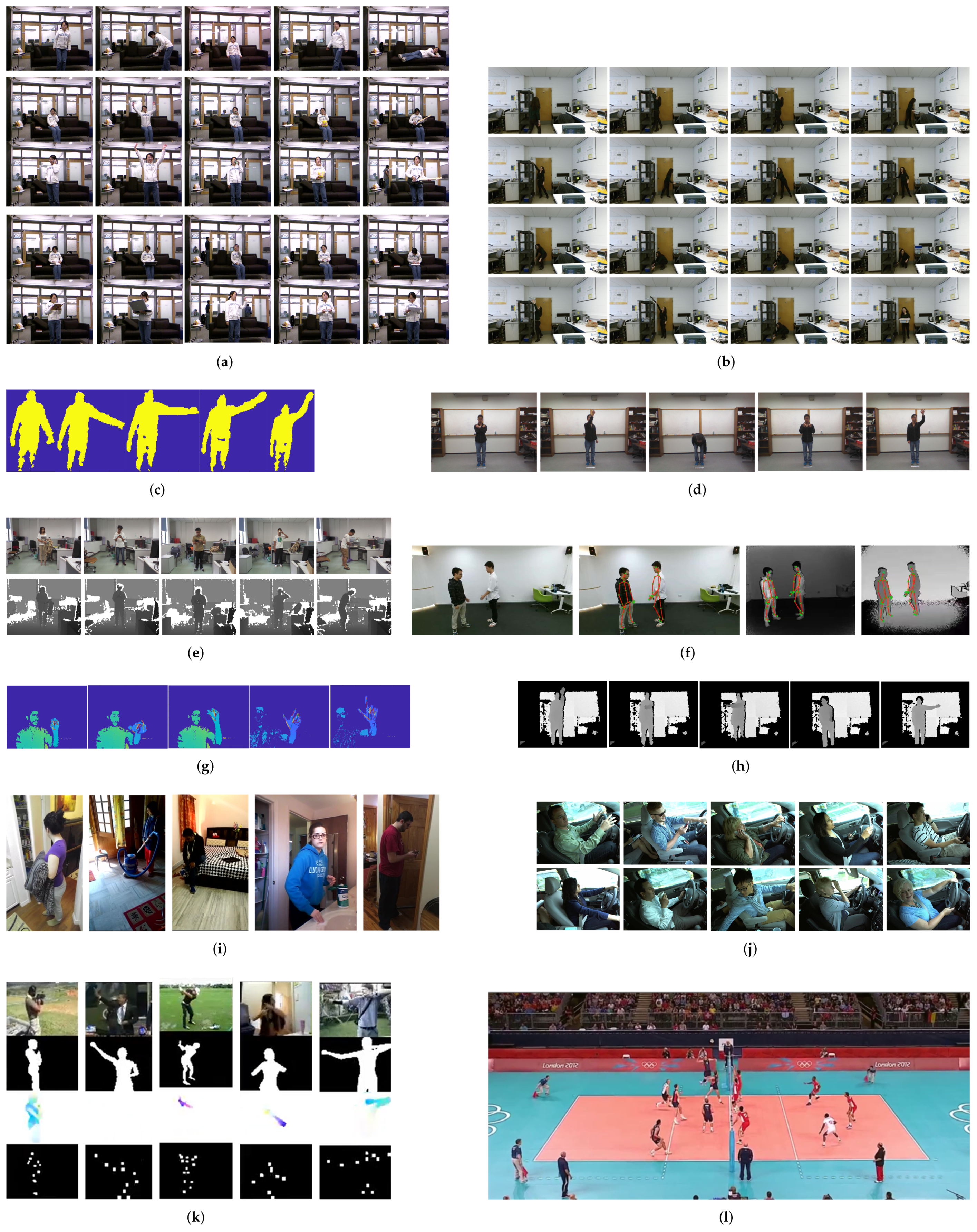
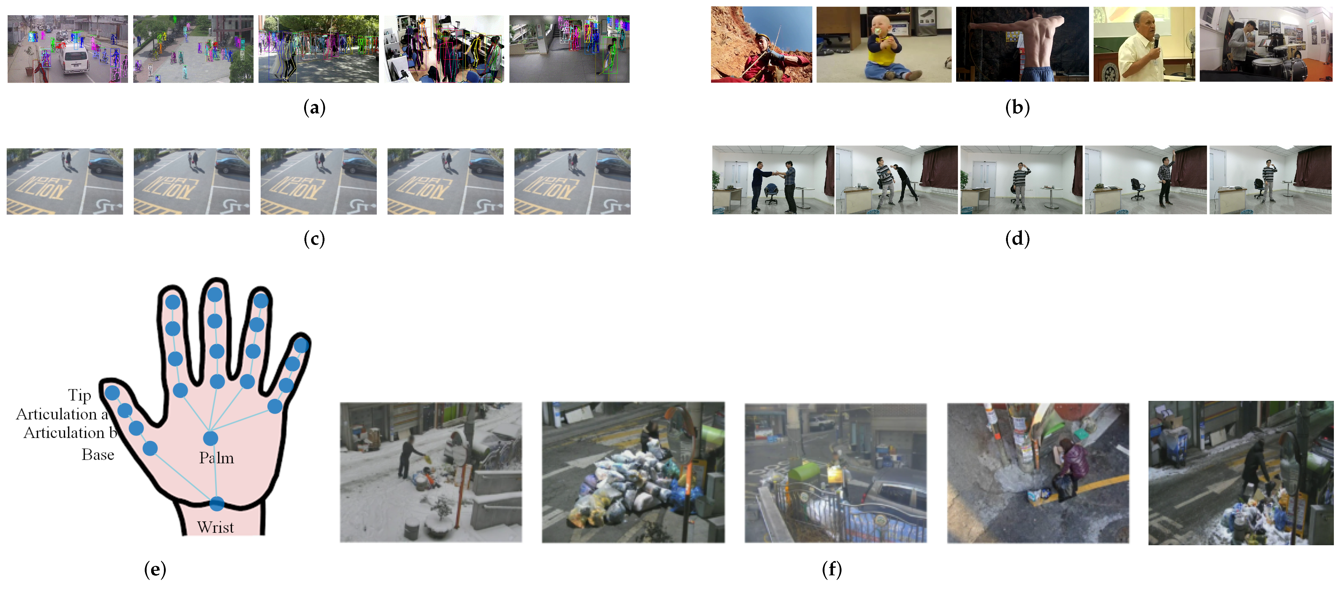
3. Skeleton Graphs in Applications
3.1. Input Graphs
3.1.1. Spatial Graphs
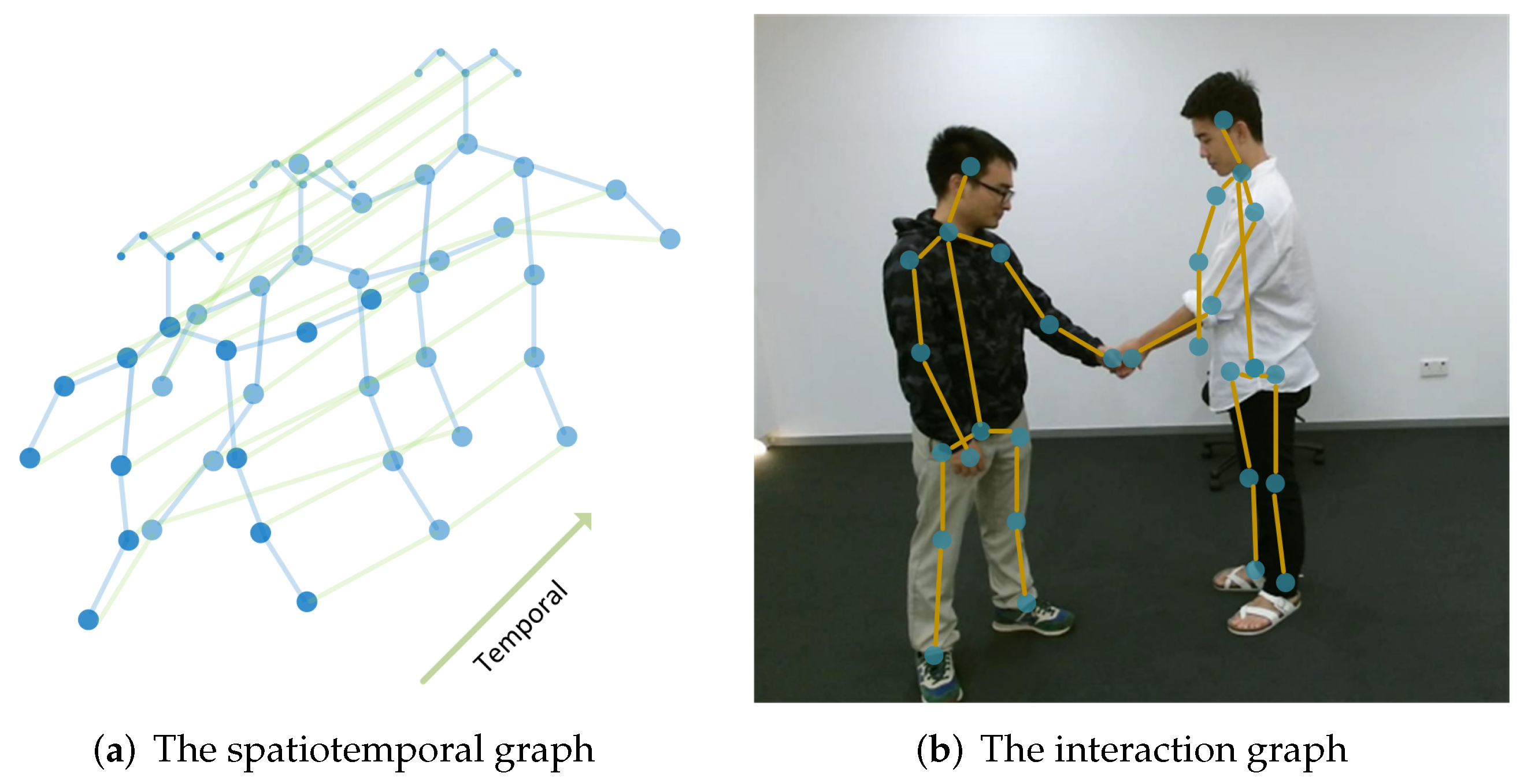
3.1.2. Spatiotemporal Graph
3.1.3. Interaction Graphs
3.1.4. Generated Graphs
3.2. Problem Definition
4. The Structure of Skeleton Graphs
4.1. Graph Structures Based on Directions
4.1.1. Undirected Graphs
4.1.2. Directed Graphs
4.2. The Construction of Graph Topology
4.2.1. Handcrafted Graph Topology
Modality Level
Frame Level
Subgraph Level
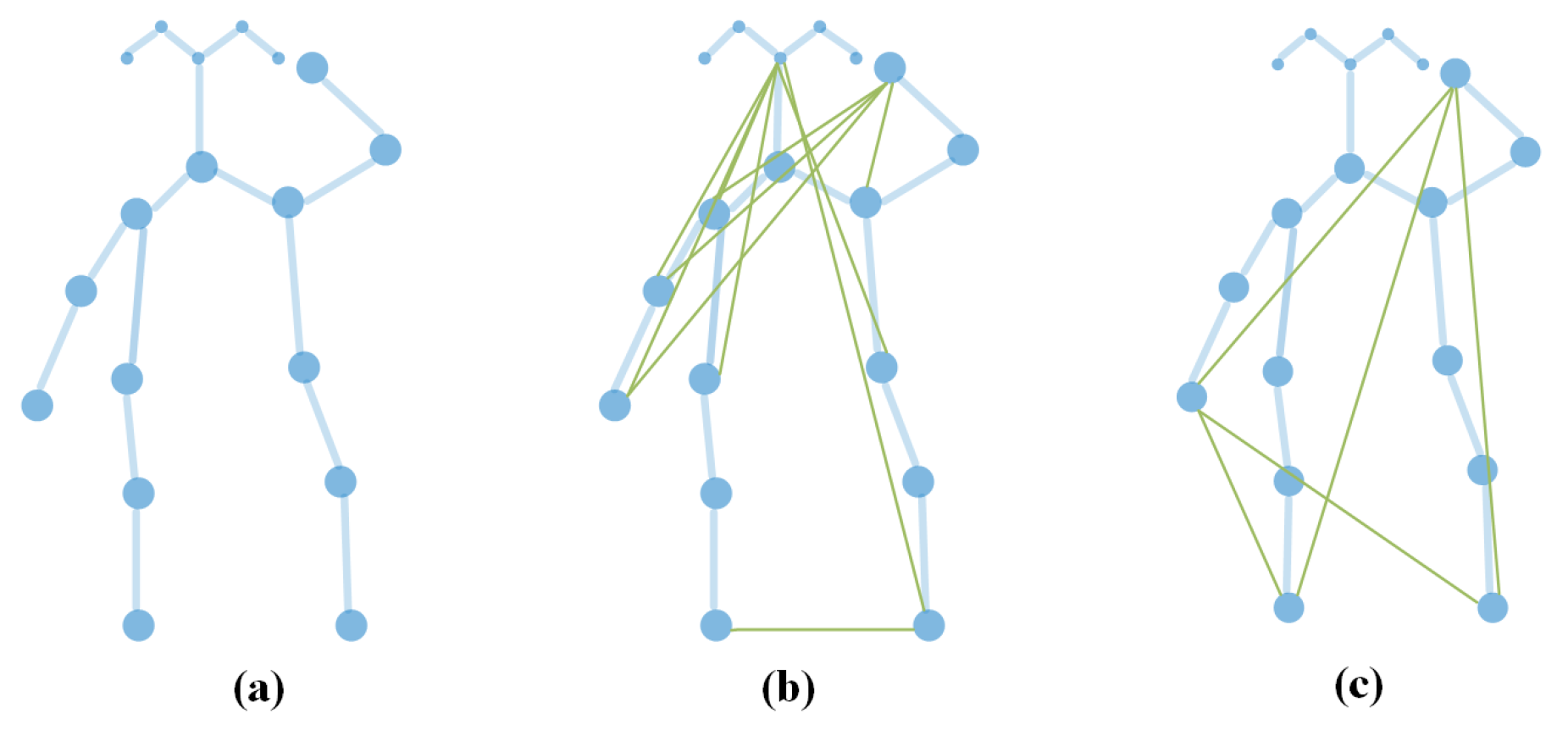
- Body-part partitionPapers, such as [56,57,58,59,60,61,62], directly divided the original skeleton graph into several body parts. Typically, the group comprising left arm, right arm, left leg, right leg and trunk, is intuitive and easy to be implemented. Normally, our limbs are more flexible than our trunk and interact more with other parts. Moreover, when people are moving, the diverse parts of the human bodies are capable of making distinct gestures. Based on this, many strategies can be designed to assign different weights strategy to these parts.
- Distance-based partitionIn this category, the definition of distance mainly focuses on centrifugal and centripetal partition, which divides the neighbors of each node into two or more parts. For one node , a node in the centripetal part is closer to the gravity center than , and a node in the centrifugal part is farther away from the gravity center than . Usually, the gravity center is the average of all skeleton joints. Although this idea does not partition the graph topology explicitly, the adjacency matrix is implicitly classified into different groups with an allowance of applying different weights.The idea was first proposed by ST-GCN that divides node ’s neighbors into the group , the group ’s centripetal joints and the group ’s centrifugal joints. The other case comes from [63], which suggests making use of neighbor bones of node and therefore augmenting the three partitions to five, with the addition of centripetal bones and centrifugal bones, where the centripetal bones are those that are closer to the gravity center than , and the centrifugal bones are those that are farther from the gravity center than .
- Multiscale partitionOne partition is based on geometry. For example, B. Parsa et al. [64] performed GNN on node-level, part-level and global-level graphs. The global level graph is the output of the group average pooling on the part-level graph, and the part-level graph is the output of group average pooling on the node-level graph (the original skeleton graph).The other partition directly makes use of downsampling so as to implement it mechanically. For example, Y. Fan et al. [65] conducted two more downsampling operations to extract additional graphs of different scales from the original graph.
Edge Level
4.2.2. Learnable Graph Topology
Frame-Level
Edge-Level
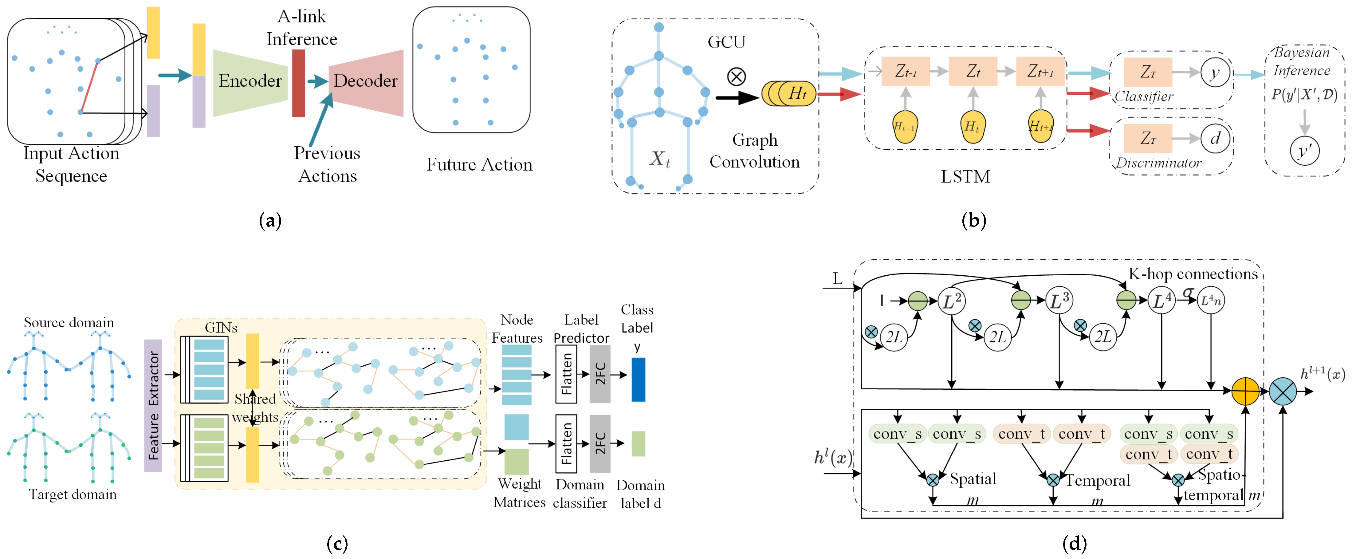
- For every three consecutive frames, X. Gao et al. [75] proposed learning a new graph with a graph regression (GR) module. The graph regression problem is formulated as the optimization of the graph Laplacian matrix . For intra-joints, the weights for weakly connected and strongly connected joints are different, where strong connections include physical connections and some physical disconnections among joints, and weak connections denote potential connections, such as those between head and hands. For the inter-joints, connections between corresponding joints along the temporal dimension and their neighborhoods are assigned with different weights, and others are set as zero.
- To capture the intrinsic high-order correlations among joints, B. Li et al. [76] proposed spatiotemporal graph routing, consisting of a spatial graph router (SGR) and temporal graph router (TGR). SGR captures the connectivity relationships among joints based on sub-group clustering. TGR focuses on structural information with the correlation degrees of joints trajectories.
- M. Li et al. [77] estimated actional links (A-links) and structural links (S-links), where A-links are estimated by encoder–decoder (AE)-based A-links inference module (AIM), and S-links are estimated by high-order polynomials of an adjacency matrix. The A-links capture the latent dependencies among joints, and S-links indicate higher order relationships.
- F. Ye et al. [78] proposed a joint relation inference network (JRIN) to aggregate the spatiotemporal features of every two joints globally and then infer the optimal relation between every two joints automatically. The relations of joints are quantified as the optimal adjacency matrices.
- F.F. Ye et al. [79] estimated edges by joint-relation-reasoning (JRR). JRR is trained by RL, optimized with policy gradient. In detail, the state equals to , where contains the global edges information, represents the connectivity weights of every tow joints, and ⊗ denotes the element-wise product; rewards comes from the output of GCN; action is the output of JRR, which indicates temporal relevance of every two joints under the current action.
- To extract the implicit connections and properly balance them for each action, W.S. Chan et al. [49] created three inference modules, namely the ratio inference, implicit edges inference and bias inference. The finally estimated matrix is the combination of the output from these three modules. The ratio of the implicit and structural edges is vital. Adjacency matrices and present the structural edges. is updated with back propagation and is kept the same for all actions.
Node-Level
- W.W. Ding et al. [83] emphasized the learning of localized correlated features. By projecting each part of human body into a node, a fully connected similarity graph is formed to capture relations among the disjoint and distant joints of the human body. The learned mapping of spatial matrices and temporal matrices can determine which part of the human body across several consecutive frames should be mapped to a node in the similarity graph.
- W.J. Yang et al. [84] merged nodes in the same part of the skeleton into one node. Each new generated node takes the weighted summation of the original nodes that it covers as its feature, using trainable weights. This integration is done part-wise and channel-wise.
- Y.X. Chen et al. [85] proposed structural pooling since the motion information contained in human body is highly related with the interaction of five body parts, and therefore graph convolution on the graph with these five-part nodes can capture more global motion information. By graph pooling, the new compressed graphs in different sizes are input to the model.
- G.M. Zhang et al. [86] proposed learning a new topology by topology-learnable graph convolution, which is decomposed as feature learning and node fusion. Node fusion is performed by a learnable fusion matrix that is initialized with a normalized adjacency matrix and added with an additional constant bias.
5. A New Taxonomy for Skeleton-GNN-Based HAR
5.1. Spatial-Based Approaches
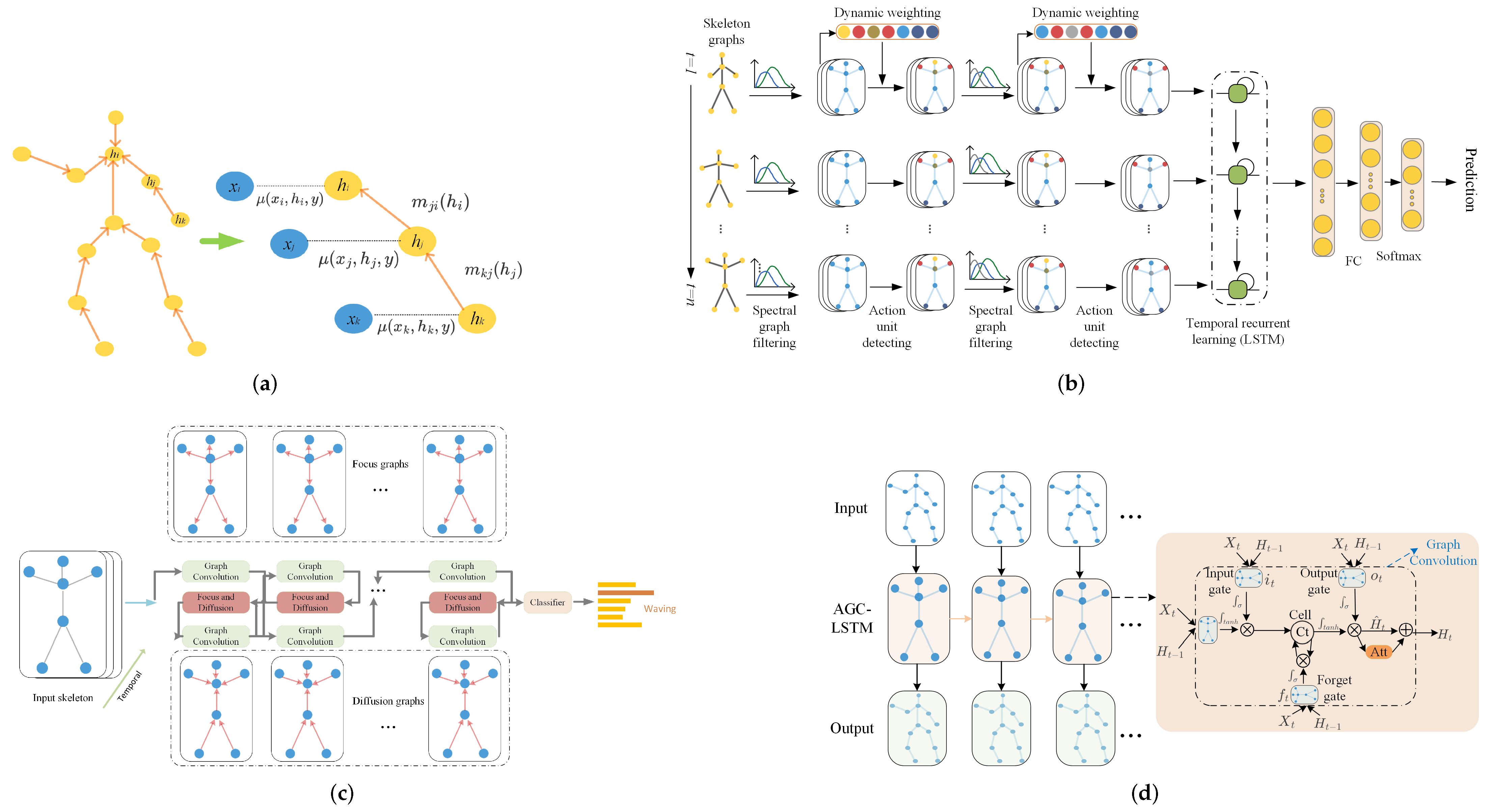
5.1.1. CRF
5.1.2. RNN
Separated Strategy
Bidirectional Strategy
Aggregated Block
5.2. Spatiotemporal Approaches
5.2.1. CNN
5.2.2. RNN
5.3. Generated Approaches
5.3.1. Self-Supervised
AE
Adversarial Learning
Teacher–Student Mechanism
5.3.2. NAS
6. The Common Frameworks
6.1. Attention Mechanism
6.1.1. Self-Attention
6.1.2. Other Attention Mechanism
Spatial Attention
- Joint-levelThe joint-level spatial attention is the most used attention module, since it helps to re-weight joints and emphasize those task-informative joints. This is especially helpful in discovering the long-distance dependency.For each channel, Y.X. Chen et al. [85] converted the the relationship between local motion pattern and global motion pattern to an attention map, where the local features come from the rescaled graph and the global features come from the original skeleton graph. This can be regarded as a channel-separated joint-wise attention.To adaptively weight skeletal joints for different human actions, C. Li et al. [88] set a dynamic attention map that works on the features from spectral GCN. This attention map varies according to the spectral GCN features and different actions, and is used to weight nodes.S. Xu et al. [92] took the point-level hidden states captured by LSTM, as the key and the query. For different people, an attention map is captured to select informative joints.X.L. Ding et al. [96,128] used the attention graph interaction module, designed to pay different levels of attention to different joints and connections. The attention map is trained together with other parameters.The other one follows the popular recipe while using LSTM, which emphasizes the informative hidden state extracted by LSTM cell. For example, C. Si et al. [89] integrated the attention operation in LSTM cells. They take the weighted summation of all nodes’ hidden states as the query, and use sigmoid similarity function to select discriminative spatial information so that to enhance the information from key joints.
- Part-levelSome researchers argue that the attention mechanism on joints is too localized and fails to detect the intra-part relation (global topologically relations).Since each action comprises of multiple interactions that happen in different parts, G. Zhang et al. [129] adopted multi-heads attention, which will generate multiple attention maps so as to focus on different parts. The attention model identifies key joints of every action by introducing two regularization terms, spatial diversity and local continuity. The spatial diversity is multi-head. It works by maximizing the distance between attention maps so as to focus on different parts. The local continuity is controlled by the attention map on graph’s Laplacian matrix.Y.F. Song et al. [119] concatenated the features of all parts and perform average pooling in temporal dimension, and then pass them through a fully connected layer with a BatchNorm layer and a ReLU function. Subsequently, five fully connected layers are adopted to calculate the attention matrices and a softmax function is utilized to determine the most essential body parts.Q.B. Zhong et al. [109] emphasized the joints with more motions and propose a novel local posture motion-based attention module (LPM-TAM) to filter out low motion information in temporal domain. This operation helps improve the ability of motion-related feature extraction. The attention map of skeleton sequence in the spatiotemporal graph is represented by the attention of local limbs estimated in temporal dimension.
Temporal Attention
Channel Attention
Auxiliary Data Attention
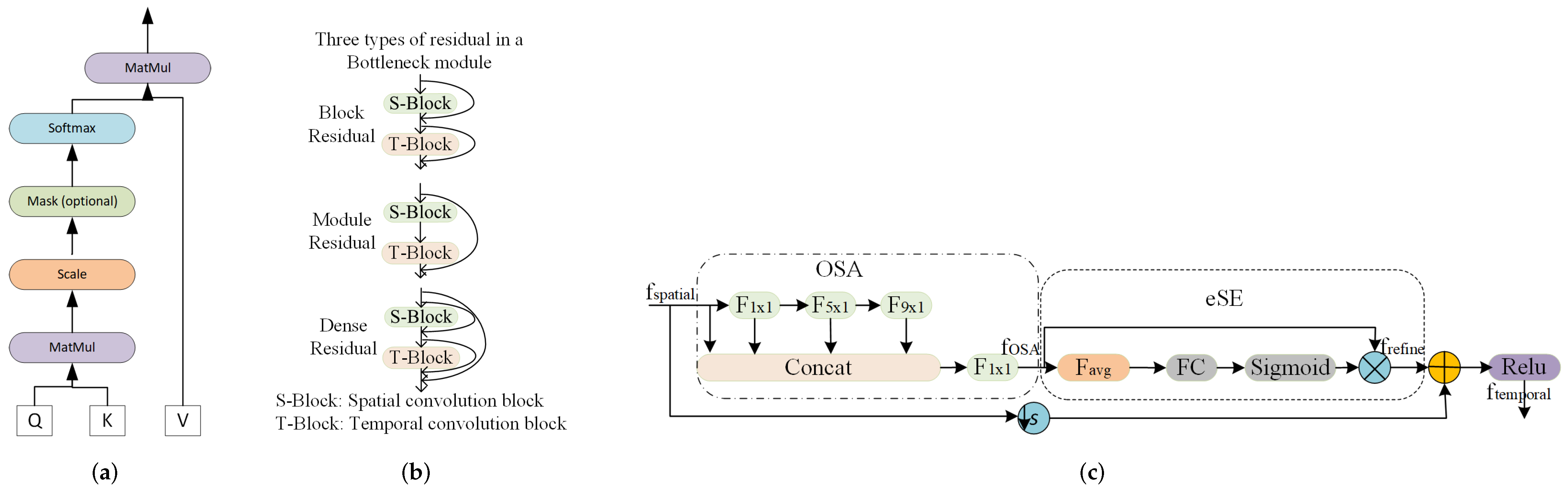
6.2. Dense Block
6.2.1. Skip Connection
6.2.2. Squeeze-and-Excitation Block
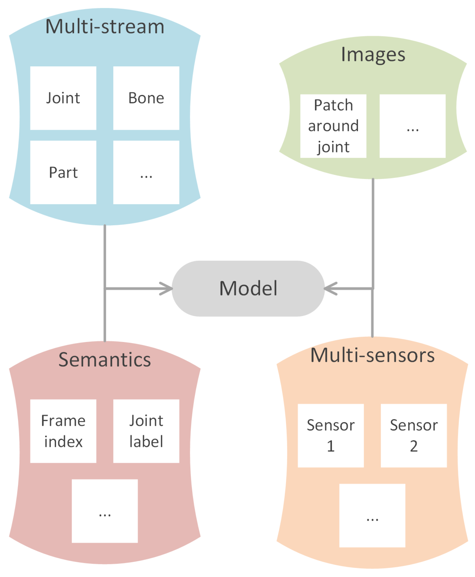
6.3. Multi-Modalities
6.3.1. Multi-Stream
6.3.2. Multi-Sensors
6.3.3. Semantics
6.3.4. Images
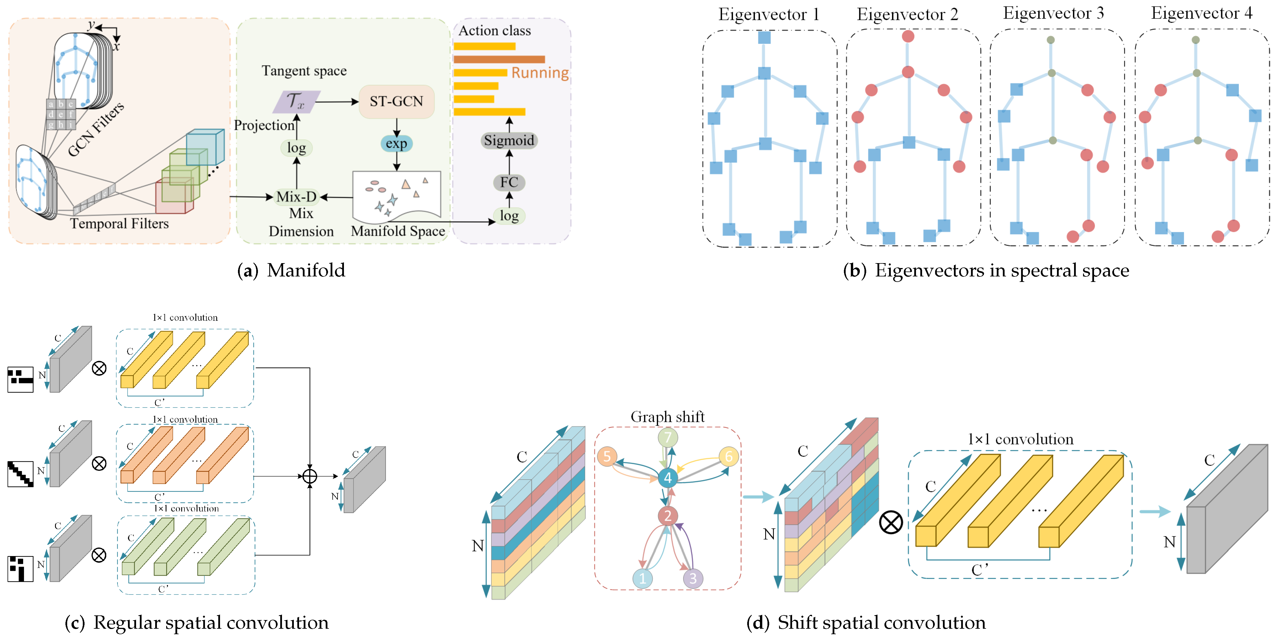
6.4. Change Feature Space
6.4.1. Manifold
6.4.2. Spectral Space
6.5. Neighbors Convolution
6.5.1. The k-Neighbors Convolution
6.5.2. Other Convolution
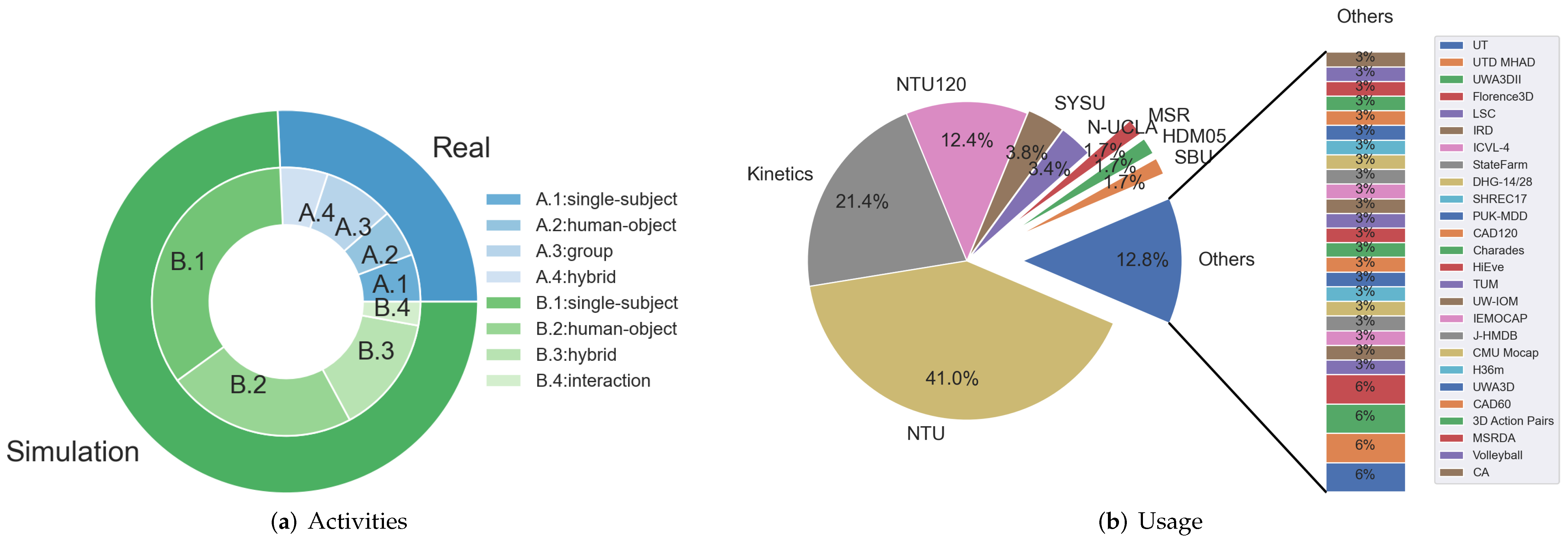
7. Datasets
7.1. Means for Collecting Datasets
7.2. Dataset Taxonomy
7.2.1. Simulation Datasets
Single-Subject Actions
Interacted Actions
Hybrid Actions
7.2.2. Real-Life Datasets
7.3. Performance
7.3.1. The Statistics of Datasets
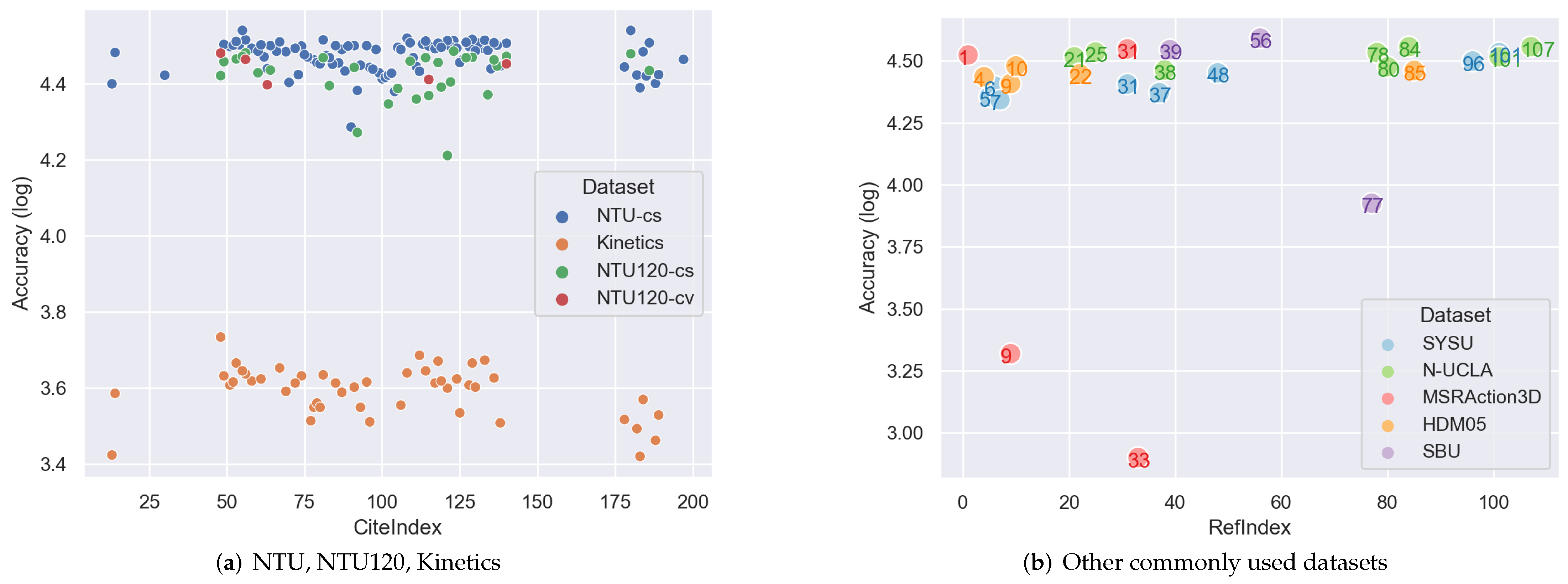
7.3.2. Model Performance
- AccuracyThe accuracy of methods is shown in Figure 14, with Figure 14a on NTU RGB+D, NTU RGB+D 120 and Kinetics, Figure 14b on SYSU, N-UCLA, MSRAction3D, HDM05 and SBU. Figure 14a demonstrates that the Kinetics dataset is more challengeable (scores are below ) than simulated NTU, considering it is a real-life dataset and only provides RGB videos. Under real-life context, because of the occlusions, illuminations, complex environments etc., it is difficult to infer 3D skeleton graphs accurately. This huge challenge proves that the accurate 3D information is neccesary for skeleton-GNN-HAR.Moreover, it is clear that cross-subjects is more challengeable than cross-views, either on NTU or NTU120. This is because 3D skeletons are view-invariant, and under cross-view case, the 3D skeletons from different view points complement each other. When skeletons are from multiple subjects, the different sizes of subjects, separated clothes etc. all contribute to increase the recognition error.On other datasets, performance on MSRAction3D varies severely. MSRAction3D is challengeable because of the 3D information without RGB videos, and high interaction similarities. Specifically, ST-GCN [13] and ST-GCN-jpd [29] underperform others [12,69], where [12] used temporal pyramid, and [69] takes LSTM as the backbone. Methods that are good at temporal tracking outperform ST-GCN-based methods. This can be explained that the temporal evolution in ST-GCN is handled by CNN.
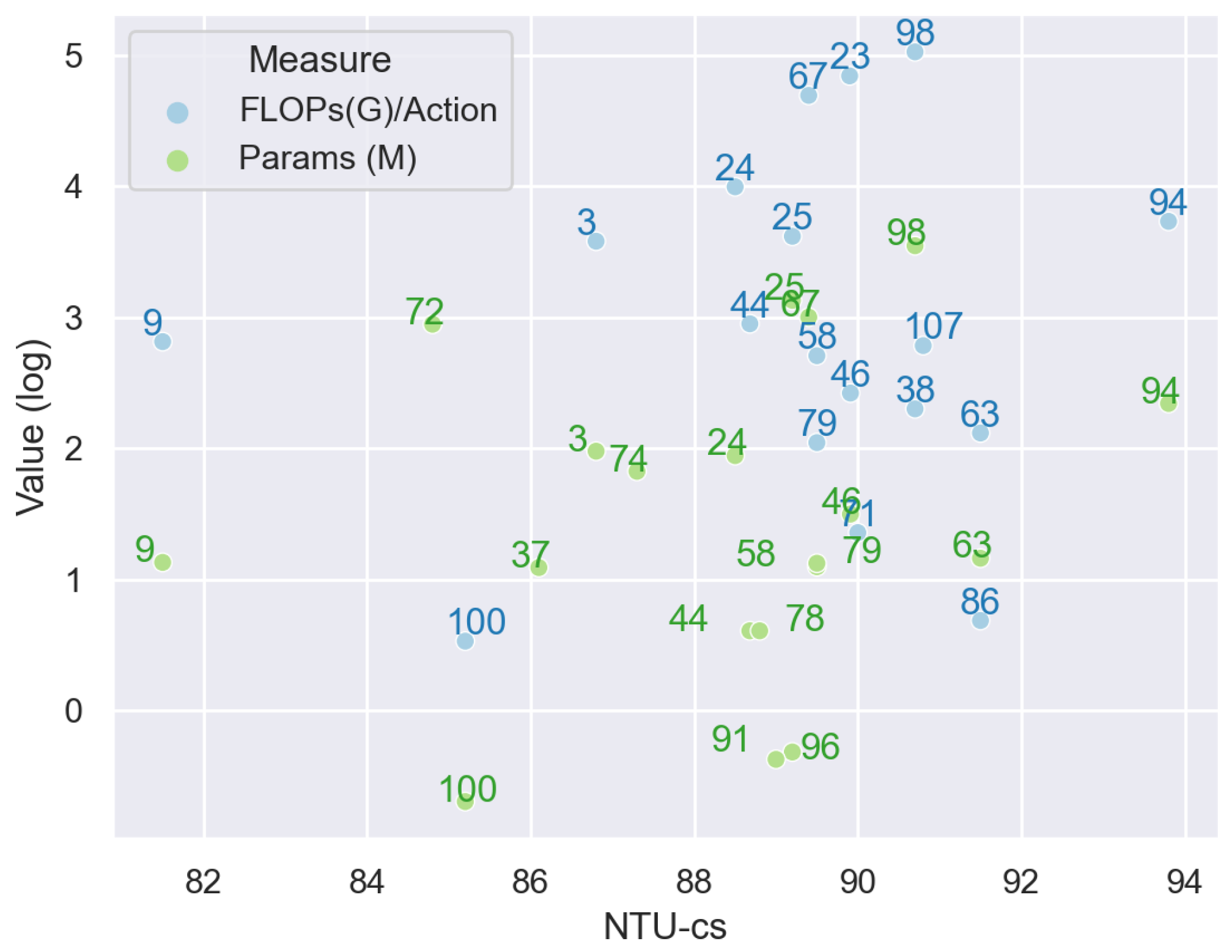
- Model Complexity and model sizeTo show the complexity and model size of each approach, the floating point operations in Gigabytes for each action sample and the size of parameters in Megabytes are collected. Because none of the mentioned papers tested all methods under the same environment, for the same approach and same dataset, these statistics vary in different papers, due to the basic assumptions, devices, platforms, counting of multi-streams, resolutions etc. Therefore, for one single approach, if the statistics are different in multiple papers, we choose the maximum value. The model complexity is measured on NTU RGB+D, collected from [54,57,80,117,121,141,180,181]. The model size is summarized from [54,55,57,82,85,117,121,135,180,181].
7.3.3. Hard Activity Cases
- Similar single subject actions without objectsFor actions involving no objects, activities are mainly misclassified due to similar motion patterns with low pose resolution or inappropriate standardized axis coordinates.When actions only differ slightly around hand joints, the low hand pose resolution will increase the classification error. For instance, the NTU RBD+D dataset only records three joints for each hand, namely the wrist, the tip of the hand and the thumb. These joints are not enough to help distinguish actions with subtle movements around hands.Therefore, for actions with subtle hand movements, the NTU skeletons are less supportive in recognition. For example, Ref. [83] observed that actions, such as rubbing two hands together and clapping, are easily confused with each other on NTU, Ref. [71] misclassified stand up as check time (from watch) on NTU, Ref. [92] mistook make victory sign as make ok sign, snapping fingers as make victory sign. Ref. [64] misclassified standing and walking especially when the back of subjects faces the camera, which is due to the low pose resolution (missing of joints) caused by self-occlusions.Authors of [64] also discovered that actions like twisting are difficult because the standardized axis coordinates (Cartesian coordinates) erases the subtle rotation around the wrist.
- Similar single subject actions with objectsSimilar human–object interactions usually differ in the subtle movements of hands and have similar action trajectories.Generally, the errors are mainly caused by low pose resolution or lacking object information.Refs. [54,91] failed while classifying reading, writing, playing with phone/tablet, and typing on a keyboard. The authors argue these actions only differ for hand movements, while the skeletons provided by NTU RGB+D are less supportive for hand joints. Ref. [114] mentioned that when the body movements are not significant, and the sizes of the objects are relatively small, e.g., counting money, and playing magic cube, and the skeletons only provide three hand joints, the model can easily become confused. Ref. [89] also blamed the low NTU hands resolution, which leads to misclassify reading as writing, writing as typing on keyboard. As for distinguishing actions with subtle movements of two hands, such as wearing a shoe, taking off a shoe, Ref. [96] failed, and expects more precise hand joints to help. Similarly, Ref. [119] made mistakes on reading and writing, and holds the same opinion for fixing it.Ref. [71] misclassified stapling book into cutting paper, counting money into playing magic cube. The authors explained that this is because the information about objects is missing. This is supported by [83], where the authors observed that although actions, such as drinking water and brushing teeth, have similar motion patterns, the objects involved are different. Ref. [89] expects that their failure cases, such as reading and writing, can be erased by combining object appearance information.
- Human–human interactionIn human–human interactions, one important reason of recognition errors given by the method set is occlusions.
8. Challenges
8.1. Pose Preparation
8.1.1. Real-Life Context
8.1.2. Pose Resolution
8.1.3. Pose Topology
8.2. View-Invariant
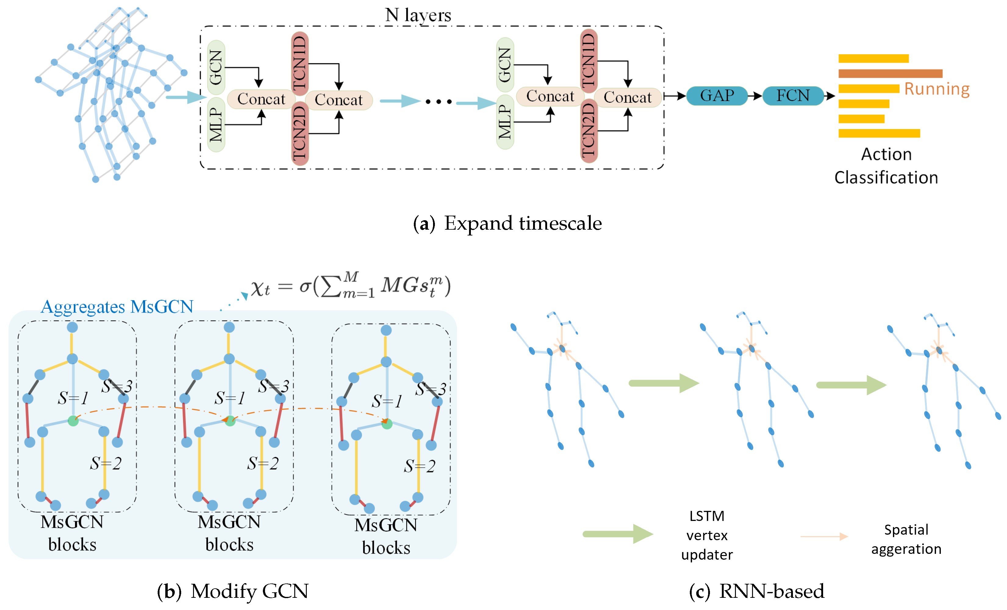
8.3. Multiscale
8.3.1. Multi Spatial Scale
8.3.2. Multi Temporal Scale
8.3.3. Multi Subject Scale
8.4. Multi-Modalities
8.4.1. Multi-Modalities Fusion
8.4.2. Inner Heterogeneous
8.5. Interactions
8.5.1. Human-Human Interaction
8.5.2. Human-Object Interaction
9. Conclusions
Author Contributions
Funding
Conflicts of Interest
Appendix A. Datasets

| Name | Sensors | Subjects | Views | Actions | Data | Year | Types |
|---|---|---|---|---|---|---|---|
| CMU Mocap, http://mocap.cs.cmu.edu/ | Vicon | 144 | - | 23 | RGB+S | 2003 | Indoor simulation, including interaction. |
| HDM05, http://resources.mpi-inf.mpg.de/HDM05/ | RRM | 5 | 6 | >70 | RGB+S | 2007 | Indoor simulation |
| IEMOCAP, https://sail.usc.edu/iemocap/ | Vicon | - | 8 | 9 | RGB+H + Script | 2008 | Emotion and speech dataset |
| CA, https://cvgl.stanford.edu/projects/collective/collectiveActivity.html | Hand held camera | - | - | 5 | RGB+PD | 2009 | Group activities |
| TUM, https://ias.in.tum.de/dokuwiki/software/kitchen-activity-data | - | - | 4 | 9 (l),9 (r), 2 (t) | RGB+S | 2009 | Activities in kitchen |
| MSR Action3D, https://sites.google.com/view/wanqingli/data-sets/msr-action3d | - | 10 | 1 | 20 | D+S | 2010 | Interaction with game consoles |
| CAD 60, https://drive.google.com/drive/folders/1Z5ztMpeys5I0XfZn8J26-_6rqplweFGI | Kinect v1 | 4 | - | 12 | RGB+D+S | 2011 | Human–object interaction |
| MSR DailyActivity3D, https://sites.google.com/view/wanqingli/data-sets/msr-dailyactivity3d | Kinect | 10 | 1 | 16 | RGB+D+S | 2012 | Daily activities in living room |
| UT-Kinect, http://cvrc.ece.utexas.edu/KinectDatasets/HOJ3D.html | Kinect v1 | 10 | 4 | 10 | RGB+D+S | 2012 | Indoor simulation |
| Florence3D, https://www.micc.unifi.it/resources/datasets/florence-3d-actions-dataset/ | Kinect v1 | 10 | - | 9 | RGB+S | 2012 | Indoor simulation |
| SBU Kinect Interaction, https://www3.cs.stonybrook.edu/~kyun/research/kinect_interaction/index.html | Kinect | 7 | - | 8 | RBB+D+S | 2012 | Human–human interaction simulation |
| J-HMDB, http://jhmdb.is.tue.mpg.de/ | HMDB51 | - | 16 | 21 | RGB+S | 2013 | Annotated subset of HMDB51, 2D skeletons, real-life |
| 3D Action Pairs, http://www.cs.ucf.edu/~oreifej/HON4D.html | Kinect v1 | 10 | 1 | 12 | RGB+D+S | 2013 | Each pair has similarity in motion and shape |
| CAD 120, https://www.re3data.org/repository/r3d100012216 | Kinect v1 | 4 | - | 10+10 | RGB+D+S | 2013 | Human–object interaction |
| ORGBD, https://sites.google.com/site/skicyyu/orgbd | - | 36 | - | 7 | RGB+D+S | 2014 | Human–object interaction |
| Human3.6M, http://vision.imar.ro/human3.6m/description.php | Laser scanner, TOF | 11 | 4 | 17 | RGB+S+M | 2014 | Indoor simulation, meshes |
| N-UCLA, http://wangjiangb.github.io/my_data.html | Kinect v1 | 10 | 3 | 10 | RGB+D+S | 2014 | Daily action simulation |
| UWA3D Multiview, https://github.com/LeiWangR/HDG | Kinect v1 | 10 | 1 | 30 | RGB+D+S | 2014 | Different scales, including self-occlusions and human–object interaction. |
| UWA3D Multiview Activity II, https://github.com/LeiWangR/HDG | Kinect v1 | 10 | 4 | 30 | RGB+D+S | 2015 | Different views and scales, including self-occlusions and human–object interaction. |
| UTD-MHAD, https://personal.utdallas.edu/~kehtar/UTD-MHAD.html | Kinect v1 + WIS | 8 | 1 | 27 | RGB+D+S | 2015 | Indoor single-subject simulation |
| NTU RGB+D, https://rose1.ntu.edu.sg/dataset/actionRecognition/ | Kinect V2 | 40 | 80 | 50 + 10 | RGB+IR +D+S | 2016 | Simulation, including human–human interaction |
| Charades, https://prior.allenai.org/projects/charades | - | 267 | - | 157 | RGB+OP | 2016 | Real-life daily indoor activities |
| UOW LSC, https://sites.google.com/view/wanqingli/data-sets/uow-largescale-combined-action3d | Kinect | - | - | 94 | RGB+D+S | 2016 | Combined dataset |
| StateFarm, https://www.kaggle.com/c/state-farm-distracted-driver-detection/data | Kaggle competition | - | - | 10 | RGB | 2016 | Real driving videos |
| DHG-14/28 | Intel RealSense | 20 | - | 14/28 | RGB+D+S | 2016 | Hand gestures |
| Volleyball, https://github.com/mostafa-saad/deep-activity-rec | YouTube volleyball | - | - | 9 | RGB | 2016 | Group activities, volleyball |
| SYSU, https://www.isee-ai.cn/~hujianfang/ProjectJOULE.html | Kinect v1 | 40 | 1 | 12 | RGB+D+S | 2017 | Human–object interaction |
| SHREC’17, http://www-rech.telecom-lille.fr/shrec2017-hand/ | Intel RealSense | 28 | - | - | RGB+D+S | 2017 | Hand gestures |
| Kinetics, https://deepmind.com/research/open-source/kinetics | YouTube | - | - | 400 | RGB | 2017 | Real life, including human–object interaction and human–human interaction |
| PUK-MDD, https://www.icst.pku.edu.cn/struct/Projects/PKUMMD.html | Kinect | 66 | 3 | 51 | RGB+D+ IR+S | 2017 | Daily action simulation, including interactions. |
| ICVL-4, https://github.com/ChengBinJin/ActionViewer | - | - | - | 13 | RGB | 2018 | Human–object action in real-life, a subset of ICVL. |
| UW-IOM, https://data.mendeley.com/datasets/xwzzkxtf9s/1 | Kinect | 20 | - | 17 | RGB+D+S | 2019 | Indoor object manipulation |
| NTU RGB+D 120, https://rose1.ntu.edu.sg/dataset/actionRecognition/ | Kinect V2 | 106 | 155 | 94 + 26 | RGB+IR + D+S | 2019 | Simulation, including human–human interaction |
| IRD | CCTV | - | - | 2 | RGB | 2019 | Illegal rubbish dumping in real life |
| HiEve, http://humaninevents.org/ | - | - | - | 14 | RGB+S | 2020 | Multi-person events under complex scenes |
| Name | Papers | Action List |
|---|---|---|
| CMU Mocap | [95] | Human Interaction, Interaction With Environment, Locomotion, Physical Activities + Sports, Situations + Scenarios |
| HDM05 | [56,61,74,88] | Walk, Run, Jump, Grab and Deposit, Sports, Sit and Lie Down, Miscellaneous Motions |
| IEMOCAP | [123] | Anger, Happiness, Excitement, Sadness, Frustration, Fear, Surprise, Other and Neutral State |
| CA | [115] | Null, Crossing, Wait, Queueing, Walk, Talk |
| TUM | [64] | Set the Table, Transport Each Object Separately as Done by an Inefficient Robot, Take Several Objects at Once as Humans Usually Do, Iteratively Pick Up and Put Down Objects From and to Different Places |
| MSR Action3D | [12,29,69,140] | High Arm Wave, Horizontal Arm Wave, Hammer, Hand Catch, Forward Punch, High Throw, Draw X, Draw Tick, Draw Circle, Hand Clap, Two Hand Wave, Side Boxing, Bend, Forward Kick, Side Kick, Jogging, Tennis Swing, Tennis Serve, Golf Swing, Pick Up + Throw |
| CAD 60 | [29] | Still, Rinse Mouth, Brush Teeth, Wear Contact Lenses, Talk on Phone, Drink Water, Open Pill Container, Cook (Chop), Cook (Stir), Talk on Couch, Relax on Couch, Write on Whiteboard, Work on Computer |
| MSR DailyActivity3D | [115] | Drink, Eat, Read Book, Call Cellphone, Write on a Paper, Use Laptop, Use Vacuum Cleaner, Cheer Up, Sit Still, Toss Paper, Play Game, Lay Down on Sofa, Walk, Play Guitar, Stand Up, Sit Down |
| UT-Kinect | [12,140] | Walk, Sit Down, Stand Up, Pick Up, Carry, Throw, Push, Pull, Wave Hands, Clap Hands |
| Florence3D | [12,88] | Wave, Drink From a Bottle, Answer Phone, Clap, Tight Lace, Sit Down, Stand Up, Read Watch, Bow |
| SBU Kinect Interaction | [83,115,182,187] | Approach, Depart, Push, Kick, Punch, Exchange Objects, Hug, and Shake Hands |
| J-HMDB | [124] | Brush Hair, Catch, Clap, Climb Stairs, Golf, Jump, Kick Ball, Pick, Pour, Pull-Up, Push, Run, Shoot Ball, Shoot Bow, Shoot Gun, Sit, Stand, Swing Baseball, Throw, Walk, Wave |
| 3D Action Pairs | [29] | Pick Up a box/Put Down a Box, Lift a box/Place a Box, Push a chair/Pull a Chair, Wear a hat/Take Off a Hat, Put on a backpack/Take Off a Backpack, Stick a poster/Remove a Poster. |
| CAD 120 | [67] | Make Cereal, Take Medicine, Stack Objects, Unstack Objects, Microwave Food, Pick Objects, Clean Objects, Take Food, Arrange Objects, Have a Meal |
| ORGBD | [115] | Drink, Eat, Use Laptop, Read Cellphone, Make Phone Call, Read Book, Use Remote |
| Human3.6M | [95] | Conversations, Eat, Greet, Talk on the Phone, Pose, Sit, Smoke, Take Photos, Wait, Walk in Various Non-Typical Scenarios (With a Hand in the Pocket, Talk on the Phone, Walk a Dog, or Buy an Item) |
| N-UCLA | [59,87,89,90,92,94,138,141] | Pick Up With One Hand, Pick Up With Two Hands, Drop Trash, Walk Around, Sit Down, Stand Up, Donning, Doffing, Throw, Carry |
| UWA3D Multiview | [29] | One Hand Wave, One Hand Punch, Sit Down, Stand Up, Hold Chest, Hold Head, Hold Back, Walk, Turn Around, Drink, Bend, Run, Kick, Jump, Mope Floor, Sneeze, Sit Down (Chair), Squat, Two Hand Wave, Two Hand Punch, Vibrate, Fall Down, Irregular Walk, Lie Down, Phone Answer, Jump Jack, Pick Up, Put Down, Dance, Cough |
| UWA3D Multiview Activity II | [29,94] | One Hand Wave, One Hand Punch, Two Hand Wave, Two Hand Punch, Sit Down, Stand Up, Vibrate, Fall Down, Hold Chest, Hold Head, Hold Back, Walk, Irregular Walk, Lie Down, Turn Around, Drink, Phone Answer, Bend, Jump Jack, Run, Pick Up, Put Down, Kick, Jump, Dance, Mope Floor, Sneeze, Sit Down (Chair), Squat, Cough |
| UTD-MHAD | [69,105] | Indoor Daily Activities. Check https://personal.utdallas.edu/~kehtar/UTD-MHAD.html for details |
| NTU RGB+D | [13,14,48,49,50,51,52,53,54,55,56,57,59,60,61,62,63,65,66,68,69,71,72,73,74,75,76,77,78,79,80,81,82,83,84,85,86,87,88,89,90,91,92,93,94,95,96,97,99,100,101,102,103,104,105,106,107,109,110,111,112,113,114,115,116,117,119,120,121,122,124,125,126,127,128,129,130,131,132,133,134,135,136,137,138,139,141,182,183,187,191,192,193,194,195,196] | https://rose1.ntu.edu.sg/dataset/actionRecognition/ |
| Charades | [67] | https://prior.allenai.org/projects/charades |
| UOW LSC | [88] | Large Motions of All Body Parts, E.g., Spinal Stretch, Raising Hands and Jumping, and Small Movements of One Part, E.g., Head Anticlockwise Circle. Check https://sites.google.com/view/wanqingli/data-Sets/uow-Largescale-Combined-Action3d for details. |
| StateFarm | [192] | Safe Drive, Text-Right, Talk on the Phone-Right, Text-Left, Talk on the Phone-Left, Operate the Radio, Drink, Reach Behind, Hair and Makeup, Talk to Passenger |
| DHG-14/28 | [70] | Grab, Tap, Expand, Pinch, Rotate Clockwise, Rotatr Couter Clockwise, Swipe Right, Swipe Left, Swipe Up, Swipe Down, Swipe X, Swipe V, Swipe +, Shake |
| Volleyball | [115] | Wait, Set, Dig, Fall, Spike, Block, Jump, Move, Stand |
| SYSU | [62,69,72,75,85,90,97,135,136] | Drink, Pour, Call Phone, Play Phone, Wear Backpacks, Pack Backpacks, Sit Chair, Move Chair, Take Out Wallet, Take From Wallet, Mope, Sweep |
| SHREC’17 | [70] | Grab, Tap, Expand, Pinch, Rotate Clockwise, Rotatr Couter Clockwise, Swipe Right, Swipe Left, Swipe Up, Swipe Down, Swipe X, Swipe V, Swipe + and Shake |
| Kinetics | [13,14,48,49,50,51,52,53,54,55,57,60,66,68,71,73,76,77,78,79,80,84,86,91,93,95,96,99,107,109,113,116,117,120,121,122,124,127,128,130,131,133,134,137,139,183,191,192,195,196] | https://deepmind.com/research/open-Source/kinetics |
| PUK-MDD | [132] | 41 Daily + 10 Interactions. Details are shown in https://www.icst.pku.edu.cn/struct/Projects/PKUMMD.html |
| ICVL-4 | [177] | Sit, Stand, Stationary, Walk, Run, Nothing, Text, and Smoke, Others |
| UW-IOM | [64] | 17 Actions as a Hierarchy Combination of four Tiers: Whether the Box or the Rod Is Manipulated, Human Motion (Walk, Stand and Bend), Captures the Type of Object Manipulation if Applicable (Reach, Pick-Up, Place and Hold) and the Relative Height of the Surface Where Manipulation Is Taking Place (Low, Medium and High) |
| NTU RGB+D 120 | [48,52,54,55,59,63,80,82,91,92,99,103,106,110,112,114,119,120,121,122,124,125,126,135,137,138,141,187,194] | 82 Daily Actions (Eating, Writing, Sitting Down etc.), 12 Health-Related Actions (Blowing Nose, Vomiting etc.) and 26 Mutual Actions (Handshaking, Pushing etc.). |
| IRD | [177] | Garbage Dump, Normal |
| HiEve | [188] | Walk-Alone, Walk-Together, Run-Alone, Run-Together, Ride, Sit-Talk, Sit-Alone, Queuing, Stand-Alone, Gather, Fight, Fall-Over, Walk-Up-Down-Stairs and Crouch-Bow |


Appendix B. Methods
| Datasets | ||||||||
|---|---|---|---|---|---|---|---|---|
| Name | Code | Year | Details | Kinetics | NTU RGB+D | NTU RGB+D 120 | ||
| CV | CS | CV | CS | |||||
| GCN [12] | - | 2017 | GCN+SVM | - | - | - | - | - |
| STGR [76] | - | 2018 | Concatenate spatial router and temporal router | 33.6 | 92.3 | 86.9 | - | - |
| AS-GCN [77] | Github | 2018 | AE, learn edges | 34.8 | 94.2 | 86.8 | - | - |
| [88] | - | 2018 | GCN+LSTM, adaptively weighting skeletal joints | - | 82.8 | 72.74 | - | - |
| GR-GCN [75] | - | 2018 | LSTM | - | 94.3 | 87.5 | - | - |
| SR-TSL [136] | - | 2018 | GCN+clip LSTM | - | 92.4 | 84.8 | - | - |
| DPRL [72] | - | 2018 | RL | - | 89.8 | 83.5 | - | - |
| BPLHM [139] | - | 2018 | Edge aggregation | 33.4 | 91.1 | 85.4 | - | - |
| ST-GCN [13] | Github | 2018 | ST-GCN | 30.7 | 88.3 | 81.5 | - | - |
| PB-GCN [61] | Github | 2018 | Skip connection, subgraphs, graphs are overlapped | - | 93.2 | 87.5 | - | - |
| 3s RA-GCN [111] | Github | 2019 | ST-GCN backbone, softmax for CAM | - | 93.5 | 85.9 | - | - |
| AR-GCN [96] | - | 2019 | Skip connection, BRNN + attentioned ST-GCN, spatial and temporal attention | 33.5 | 93.2 | 85.1 | - | - |
| GVFE+AS-GCN with DH-TCN [112] | - | 2019 | ST-GCN-based, dilated temporal CNN, skip connection | - | 92.8 | 85.3 | - | 78.3 |
| BAGCN [53] | - | 2019 | LSTM | - | 96.3 | 90.3 | - | - |
| [101] | - | 2019 | ST-GCN | - | 89.6 | 82.6 | - | - |
| [140] | - | 2019 | GFT | - | - | - | - | - |
| OHA-GCN [177] | - | 2019 | Human–object, frame selection + GCN | - | - | - | - | - |
| AM-STGCN [191] | - | 2019 | Attention | 32.9 | 91.4 | 83.4 | - | - |
| [192] | - | 2019 | GCN | 30.59 | 88.87 | 80.66 | - | - |
| [70] | - | 2019 | Add edges, hand gestures | - | - | - | - | - |
| GCN-HCRF [87] | - | 2019 | HCRF, directed message passing | - | 91.7 | 84.3 | - | - |
| Si-GCN [56] | - | 2019 | Structure induced part-graphs | - | 89.05 | 84.15 | - | - |
| 4s DGNN [50] | Github | 2019 | Directed graph | 36.9 | 96.1 | 89.9 | - | - |
| 2s-AGCN [14] | Github | 2019 | Two stream, attention | 36.1 | 95.1 | 88.5 | - | - |
| 2s AGC-LSTM [89] | - | 2019 | Attention | - | 95.0 | 89.2 | - | - |
| SDGCN [133] | - | 2019 | Skip connection | - | 95.74 | 89.58 | - | - |
| JRIN-SGCN [78] | - | 2019 | Adjacent inference | 35.2 | 91.9 | 86.2 | - | - |
| JRR-GCN [79] | - | 2019 | RL for joint-relation-reasoning | 34.8 | 91.2 | 85.89 | - | - |
| 3heads-MA-GCN [129] | - | 2019 | Multi-heads attention | - | 91.5 | 86.9 | - | - |
| GC-LSTM [98] | - | 2019 | LSTM | - | 92.3 | 83.9 | - | - |
| Bayesian GC-LSTM [69] | - | 2019 | Bayesian for the parameters of GC-LSTM | - | 89 | 81.8 | - | - |
| RGB + skeleton [113] | - | 2020 | Cross attention (joints + scenario context information), ST-GCN backbone | 39.9 | 89.27 | 84.23 | - | - |
| ST-GCN-jpd [29] | - | 2020 | ST-GCN backbone | - | 88.84 | 83.36 | - | - |
| [132] | - | 2020 | Skip connection, attention to select joints | - | - | 90.7 | - | - |
| 2s-FGCN [68] | - | 2020 | Fully connected graph | 36.3 | 95.6 | 88.7 | - | - |
| 2s-GAS-GCN [49] | - | 2020 | Gated CNN, channel attention | 37.8 | 96.5 | 90.4 | - | 86.4 |
| SGP-JCA-GCN [85] | - | 2020 | Structure-based graph pooling, learn edges between human parts | - | 93.1 | 86.1 | - | - |
| 4s Shift-GCN [141] | Github | 2020 | Cheap computation, shift graph convolution | - | 96.5 | 90.7 | 85.9 | 87.6 |
| STG-INs [83] | - | 2020 | LSTM | - | 88.7 | 85.8 | - | - |
| MS-AGCN [114] | - | 2020 | Multistream, AGCN backbone | - | 95.8 | 90.5 | - | - |
| MSGCN [65] | - | 2020 | Attention+SE block, scaled by part division | - | 95.7 | 88.8 | - | - |
| Res-split GCN [51] | - | 2020 | Directed graph, skip connection | 37.2 | 96.2 | 90.2 | - | - |
| Stacked-STGCN [67] | - | 2020 | Hourglass, human–object-scene nodes | - | - | - | - | - |
| 2s-PST-GCN [117] | - | 2020 | Find new topology | 35.53 | 95.1 | 88.68 | - | - |
| 2s-ST-BLN [81] | - | 2020 | Symmetric spatial attention, symmetric of relative positions of joints | - | 95.1 | 87.8 | - | - |
| 4s-TA-GCN [130] | - | 2020 | Skip connection, temporal attention | 36.9 | 95.8 | 89.91 | - | - |
| DAG-GCN [100] | - | 2020 | Joint and channel attention, build dependence relations for bone nodes | - | 95.76 | 90.01 | 82.44 | 79.03 |
| LSGM+GTSC [97] | - | 2020 | LSTM, feature calibration, temporal attention | - | 91.74 | 84.71 | - | - |
| VT+GARN (Joint&Part) [94] | - | 2020 | View-invariant, RNN | - | - | - | - | - |
| [102] | - | 2020 | Skeleton fusion, ST-GCN backbone | - | - | 82.9 | - | - |
| 4s-EE-GCN [120] | - | 2020 | One-shot aggregation, CNN | 39.1 | 96.8 | 91.6 | - | 87.4 |
| MS-ESTGCN [134] | - | 2020 | Spatial conv. + temporal conv. | 39.4 | 96.8 | 91.4 | - | - |
| EN-GCN [193] | - | 2020 | Fuse edge and node | - | 91.6 | 83.2 | - | - |
| MS TE-GCN [194] | - | 2020 | GCN+1DCNN as TCN | - | 96.2 | 90.8 | - | 84.4 |
| ST-GCN+channel augmentation [103] | - | 2020 | ST-GCN+new features from parameterized curve | - | 91.3 | 83.4 | - | 77.3 |
| RHCN+ACSC + STUFE [182] | - | 2020 | CNN, skeleton alignment | - | 92.5 | 86.9 | - | - |
| [188] | - | 2020 | Use MS-G3D to extract features, multiple person | - | - | - | - | - |
| MS-TGN [57] | - | 2020 | Multi-scale graph | 37.3 | 95.9 | 89.5 | - | - |
| MM-IGCN [126] | - | 2020 | Attention, skip connection, TCN | - | 96.7 | 91.3 | - | 88.8 |
| SlowFast-GCN [104] | - | 2020 | Two stream with 2 temporal resolution, ST-GCN backbone | - | 90.0 | 83.8 | - | - |
| VE-GCN [63] | - | 2020 | CRF as loss, distance-based partition, learn edges | - | 95.2 | 90.1 | - | 84.5 |
| RV-HS-GCNs [187] | - | 2020 | GCN, interaction representaion | - | 96.61 | 93.79 | - | 88.2 |
| MS-G3D [55] | Github | 2020 | Dialted window, GCN+TCN | 38 | 96.2 | 91.5 | 86.9 | 88.4 |
| WST-GCN [105] | - | 2020 | Multi ST-GCN, ranking loss | - | 89.8 | 79.9 | - | - |
| MS-AAGCN+TEM [66] | - | 2020 | Extended TCN as TEM | 38.6 | 96.5 | 91 | - | - |
| ST-PGN [64] | - | 2020 | GRU, PGNs+LSTM | - | - | - | - | - |
| GCN-NAS [116] | Github | 2020 | GRU, PGNs, LSTM | 37.1 | 95.7 | 89.4 | - | - |
| Poincare-GCN [106] | - | 2020 | ST-GCN on Poincare space | - | 96 | 89.7 | - | 80.5 |
| ST-TR [125] | Github | 2020 | Spatial self-attention + temporal self-attention | - | 96.1 | 89.9 | - | 81.9 |
| S-STGCN [123] | - | 2020 | Skip connection, self-attention | - | - | - | - | - |
| MS-AAGCN [73] | Github | 2020 | Attention | 37.8 | 96.2 | 90 | - | - |
| HSR-TSL [62] | - | 2020 | Skip connection, skip-clip LSTM | - | 92.4 | 84.8 | - | - |
| PA-ResGCN [119] | Github | 2020 | Part attention | - | 96.0 | 90.9 | - | 87.3 |
| 3s RA-GCN [82] | Github | 2020 | Occlusion, select joints, ST-GCN backbone | - | 93.6 | 87.3 | - | 81.1 |
| IE-GCN [107] | - | 2020 | L-hop neighbours, skip connection, ST-GCN backbone | 35.0 | 95.0 | 89.2 | - | - |
| FV-GNN [195] | - | 2020 | FV encoding, ST-GCN as feature extractor | 31.9 | 89.8 | 81.6 | - | - |
| GINs [115] | - | 2020 | Two skeletons, transfer learning (teacher–student) | - | - | - | - | - |
| MV-IGNet [59] | Github | 2020 | Two graphs, multi-scale graph | - | 96.1 | 88.8 | - | 83.9 |
| GCLS [127] | - | 2020 | Spatial attention, channel attention | 37.5 | 96.1 | 89.5 | - | - |
| AMCGC-LSTM [92] | - | 2020 | LSTM, point, joint and scene level transformation | - | 87.6 | 80.1 | - | 71.7 |
| GGCN+FSN [91] | - | 2020 | RL, TCN, feature fusion based on LSTM | 36.7 | 95.7 | 90.1 | - | 85.1 |
| ST-GCN-PAM [48] | Github | 2020 | Pairwise adjacency, ST-GCN backbone interaction | 41.68 | - | - | 76.85 | 73.87 |
| CGCN [60] | - | 2020 | ST-GCN backbone | 37.5 | 96.4 | 90.3 | - | - |
| FGCN [138] | - | 2020 | Dense connnection of GCN layers | - | 96.3 | 90.2 | - | 85.4 |
| PGCN-TCA [74] | - | 2020 | Learn graph connections, spatial+channel attention | - | 93.6 | 88.0 | - | - |
| Dynamic GCN [80] | - | 2020 | Seperable CNN as CeN to regress adjacency matrix | 37.9 | 96.0 | 91.5 | - | 87.3 |
| PeGCN [93] | Github | 2020 | AGCN backbone | 34.8 | 93.4 | 85.6 | - | - |
| CA-GCN [196] | - | 2020 | Directed graph, vertex information aggregation | 34.1 | 91.4 | 83.5 | - | - |
| SFAGCN [99] | - | 2020 | Gated TCN | 38.3 | 96.7 | 91.2 | - | 87.3 |
| 2s-AGCN+PM-STFGCN [109] | - | 2020 | Attetion, AGCN/ST-GCN backbone | 38.1 | 96.5 | 91.9 | - | - |
| 2s-TL-GCN [86] | - | 2020 | d-distance adjacency matrix, ST-GCN/AGCN backbone | 36.2 | 95.4 | 89.2 | - | - |
| 2s-WPGCN [52] | - | 2020 | 5-parts directed subgraph, GCN backbone | 39.1 | 96.5 | 91.1 | - | 87.0 |
| SAGP [124] | - | 2020 | Attention, spectral sparse graph | 36.6 | 96.9 | 91.3 | - | 67.5 |
| JOLO-GCN (2s-AGCN) [54] | - | 2020 | Descriptor of motion, ST-GCN/AGCN backbone | 38.3 | 98.1 | 93.8 | - | 87.6 |
| Sem-GCN [128] | - | 2020 | Attention, skip connection, L-hop, semantics | 34.3 | 94.2 | 86.2 | - | - |
| SGN [135] | Github | 2020 | Use semantics (frame + joint index) | - | 94.5 | 89.0 | - | 79.2 |
| Hyper-GNN [71] | - | 2021 | Add hyperedges, attention, skip connection | 37.1 | 95.7 | 89.5 | - | - |
| SEFN [121] | - | 2021 | Multi-perspective Attention, AGC+TGC block | 39.3 | 96.4 | 90.7 | - | 86.2 |
| Sym-GNN [95] | - | 2021 | Multiple graph, one-hop, GRU | 37.2 | 96.4 | 90.1 | - | - |
| PR-GCN [183] | Github | 2021 | MCNN, attention, pose refinement | 33.7 | 91.7 | 85.2 | - | - |
| GCN-HCRF [90] | - | 2021 | HCRF | - | 95.5 | 90.0 | - | - |
| 2s-ST-GDN [122] | - | 2021 | GDN, part-wise attention | 37.3 | 95.9 | 89.7 | - | 80.8 |
| STV-GCN [198] | - | 2021 | ST-GCN to obtain emotional state, KNN | - | - | - | - | - |
| MMDGCN [137] | - | 2021 | Dense GCN, ST-attention | 37.6 | 96.5 | 90.8 | - | 86.8 |
| CC-GCN [131] | - | 2021 | CNN, generate new graph | 36.7 | 95.33 | 88.87 | - | - |
| SGCN-CAMM [84] | - | 2021 | GCN, redundancies, merge nodes by weighted summation of original nodes | 37.1 | 96.2 | 90.1 | - | - |
| DCGCN [110] | Github | 2021 | ST-GCN backbone, attentioned graph dropout | - | 96.6 | 90.8 | - | 86.5 |
References
- Aggarwal, J.K.; Ryoo, M.S. Human activity analysis: A review. ACM Comput. Surv. (CSUR) 2011, 43, 1–43. [Google Scholar] [CrossRef]
- Ziaeefard, M.; Bergevin, R. Semantic human activity recognition: A literature review. Pattern Recognit. 2015, 48, 2329–2345. [Google Scholar] [CrossRef]
- Meng, M.; Drira, H.; Boonaert, J. Distances evolution analysis for online and off-line human object interaction recognition. Image Vis. Comput. 2018, 70, 32–45. [Google Scholar] [CrossRef] [Green Version]
- Zhang, W.; Liu, Z.; Zhou, L.; Leung, H.; Chan, A.B. Martial arts, dancing and sports dataset: A challenging stereo and multi-view dataset for 3d human pose estimation. Image Vis. Comput. 2017, 61, 22–39. [Google Scholar] [CrossRef]
- Panwar, M.; Mehra, P.S. Hand gesture recognition for human computer interaction. In Proceedings of the 2011 International Conference on Image Information Processing, Shimla, India, 3–5 November 2011; pp. 1–7. [Google Scholar]
- Sagayam, K.M.; Hemanth, D.J. Hand posture and gesture recognition techniques for virtual reality applications: A survey. Virtual Real. 2017, 21, 91–107. [Google Scholar] [CrossRef]
- Schröder, M.; Ritter, H. Deep learning for action recognition in augmented reality assistance systems. In Proceedings of the ACM SIGGRAPH 2017 Posters, Los Angeles, CA, USA, 30 July–3 August 2017; pp. 1–2. [Google Scholar]
- Bates, T.; Ramirez-Amaro, K.; Inamura, T.; Cheng, G. On-line simultaneous learning and recognition of everyday activities from virtual reality performances. In Proceedings of the 2017 IEEE/RSJ International Conference on Intelligent Robots and Systems (IROS), Vancouver, BC, Canada, 24–28 September 2017; pp. 3510–3515. [Google Scholar]
- Meng, H.; Pears, N.; Bailey, C. A human action recognition system for embedded computer vision application. In Proceedings of the 2007 IEEE Conference on Computer Vision and Pattern Recognition, Minneapolis, MN, USA, 17–22 June 2007; pp. 1–6. [Google Scholar]
- Beddiar, D.R.; Nini, B.; Sabokrou, M.; Hadid, A. Vision-based human activity recognition: A survey. Multimed. Tools Appl. 2020, 79, 30509–30555. [Google Scholar] [CrossRef]
- Yang, X.; Tian, Y.L. Eigenjoints-based action recognition using naive-bayes-nearest-neighbor. In Proceedings of the 2012 IEEE Computer Society Conference on Computer Vision and Pattern Recognition Workshops, Providence, RI, USA, 16–21 June 2012; pp. 14–19. [Google Scholar]
- Li, M.; Leung, H. Graph-based approach for 3D human skeletal action recognition. Pattern Recognit. Lett. 2017, 87, 195–202. [Google Scholar] [CrossRef]
- Yan, S.; Xiong, Y.; Lin, D. Spatial temporal graph convolutional networks for skeleton-based action recognition. In Proceedings of the AAAI Conference on Artificial Intelligence, New Orleans, LA, USA, 2–7 February 2018; Volume 32. [Google Scholar]
- Shi, L.; Zhang, Y.; Cheng, J.; Lu, H. Two-stream adaptive graph convolutional networks for skeleton-based action recognition. In Proceedings of the IEEE/CVF Conference on Computer Vision and Pattern Recognition, Long Beach, CA, USA, 16–20 June 2019; pp. 12026–12035. [Google Scholar]
- Hamilton, W.L. Graph representation learning. Synth. Lect. Artif. Intell. Mach. Learn. 2020, 14, 1–159. [Google Scholar] [CrossRef]
- Gori, M.; Monfardini, G.; Scarselli, F. A new model for learning in graph domains. In Proceedings of the 2005 IEEE International Joint Conference on Neural Networks, Montreal, QC, Canada, 31 July–4 August 2005; Volume 2, pp. 729–734. [Google Scholar]
- Ahad, M.A.R.; Tan, J.; Kim, H.; Ishikawa, S. Action dataset — A survey. In Proceedings of the SICE Annual Conference 2011, Tokyo, Japan, 13–18 September 2011; pp. 1650–1655. [Google Scholar]
- Hassner, T. A Critical Review of Action Recognition Benchmarks. In Proceedings of the 2013 IEEE Conference on Computer Vision and Pattern Recognition Workshops, Portland, OR, USA, 23–28 June 2013; pp. 245–250. [Google Scholar] [CrossRef]
- Baisware, A.; Sayankar, B.; Hood, S. Review on Recent Advances in Human Action Recognition in Video Data. In Proceedings of the 2019 9th International Conference on Emerging Trends in Engineering and Technology—Signal and Information Processing (ICETET-SIP-19), Nagpur, India, 1–2 November 2019; pp. 1–5. [Google Scholar] [CrossRef]
- Zhang, N.; Wang, Y.; Yu, P. A Review of Human Action Recognition in Video. In Proceedings of the 2018 IEEE/ACIS 17th International Conference on Computer and Information Science (ICIS), San Francisco Marriott Marquis, San Francisco, CA, USA, 13–16 December 2018; pp. 57–62. [Google Scholar] [CrossRef]
- Dhamsania, C.J.; Ratanpara, T.V. A survey on Human action recognition from videos. In Proceedings of the 2016 Online International Conference on Green Engineering and Technologies (IC-GET), Online, 19 November 2016; pp. 1–5. [Google Scholar] [CrossRef]
- Zhang, H.B.; Zhang, Y.X.; Zhong, B.; Lei, Q.; Yang, L.; Du, J.X.; Chen, D.S. A Comprehensive Survey of Vision-Based Human Action Recognition Methods. Sensors 2019, 19, 1005. [Google Scholar] [CrossRef] [Green Version]
- Wu, D.; Sharma, N.; Blumenstein, M. Recent advances in video-based human action recognition using deep learning: A review. In Proceedings of the 2017 International Joint Conference on Neural Networks (IJCNN), Anchorage, AK, USA, 14–19 May 2017; pp. 2865–2872. [Google Scholar] [CrossRef]
- Han, F.; Reily, B.; Hoff, W.; Zhang, H. Space-time representation of people based on 3D skeletal data: A review. Comput. Vis. Image Underst. 2017, 158, 85–105. [Google Scholar] [CrossRef] [Green Version]
- Lo Presti, L.; La Cascia, M. 3D skeleton-based human action classification: A survey. Pattern Recognit. 2016, 53, 130–147. [Google Scholar] [CrossRef]
- Ren, B.; Liu, M.; Ding, R.; Liu, H. A survey on 3d skeleton-based action recognition using learning method. arXiv 2020, arXiv:2002.05907. [Google Scholar]
- Chen, C.; He, B.; Zhang, H. Review on Human Action Recognition. In Proceedings of the 2017 International Conference on Computer Technology, Electronics and Communication (ICCTEC), Dalian, China, 19–21 December 2017; pp. 75–81. [Google Scholar] [CrossRef]
- Majumder, S.; Kehtarnavaz, N. Vision and Inertial Sensing Fusion for Human Action Recognition: A Review. IEEE Sens. J. 2021, 21, 2454–2467. [Google Scholar] [CrossRef]
- Wang, L.; Huynh, D.; Koniusz, P. A Comparative Review of Recent Kinect-Based Action Recognition Algorithms. IEEE Trans. Image Process. 2020, 29, 15–28. [Google Scholar] [CrossRef] [Green Version]
- Liang, B.; Zheng, L. A Survey on Human Action Recognition Using Depth Sensors. In Proceedings of the 2015 International Conference on Digital Image Computing: Techniques and Applications (DICTA), Adelaide, Australia, 23–25 November 2015; pp. 1–8. [Google Scholar] [CrossRef]
- Schwickert, L.; Becker, C.; Lindemann, U.; Marechal, C.; Bourke, A.; Chiari, L.; Helbostad, J.L.; Zijlstra, W.; Aminian, K.; Todd, C.; et al. Fall detection with body-worn sensors A systematic review. Z. Fur Gerontol. Und Geriatr. 2013, 46, 706–719. [Google Scholar] [CrossRef]
- Ahmad, T.; Jin, L.; Zhang, X.; Lin, L.; Tang, G. Graph Convolutional Neural Network for Human Action Recognition: A Comprehensive Survey. IEEE Trans. Artif. Intell. 2021, 2, 128–145. [Google Scholar] [CrossRef]
- Karthickkumar, S.; Kumar, K. A survey on Deep learning techniques for human action recognition. In Proceedings of the 2020 International Conference on Computer Communication and Informatics (ICCCI), Da Nang, Vietnam, 30 November–3 December 2020; pp. 1–6. [Google Scholar] [CrossRef]
- Zhang, Z.; Ma, X.; Song, R.; Rong, X.; Tian, X.; Tian, G.; Li, Y. Deep learning based human action recognition: A survey. In Proceedings of the 2017 Chinese Automation Congress (CAC), Jinan, China, 20–22 October 2017; pp. 3780–3785. [Google Scholar] [CrossRef]
- Qi, Z. A Review on Action Recognition and Its Development Direction. In Proceedings of the 2020 International Conference on Computing and Data Science (CDS), Stanford, CA, USA, 1–2 August 2020; pp. 338–342. [Google Scholar] [CrossRef]
- Yao, G.L.; Lei, T.; Zhong, J.D. A review of Convolutional-Neural-Network-based action recognition. Pattern Recognit. Lett. 2019, 118, 14–22. [Google Scholar] [CrossRef]
- Gao, Z.M.; Wang, P.C.; Wang, H.G.; Xu, M.L.; Li, W.Q. A Review of Dynamic Maps for 3D Human Motion Recognition Using ConvNets and Its Improvement. Neural Process. Lett. 2020, 52, 1501–1515. [Google Scholar] [CrossRef]
- Sargano, A.B.; Angelov, P.; Habib, Z. A Comprehensive Review on Handcrafted and Learning-Based Action Representation Approaches for Human Activity Recognition. Appl. Sci. 2017, 7, 110. [Google Scholar] [CrossRef] [Green Version]
- Lei, Q.; Du, J.X.; Zhang, H.B.; Ye, S.; Chen, D.S. A Survey of Vision-Based Human Action Evaluation Methods. Sensors 2019, 19, 4129. [Google Scholar] [CrossRef] [Green Version]
- Ji, Y.; Yang, Y.; Shen, F.; Shen, H.T.; Li, X. A Survey of Human Action Analysis in HRI Applications. IEEE Trans. Circuits Syst. Video Technol. 2020, 30, 2114–2128. [Google Scholar] [CrossRef]
- Chen, L.; Ma, N.; Wang, P.; Li, J.; Wang, P.; Pang, G.; Shi, X. Survey of pedestrian action recognition techniques for autonomous driving. Tsinghua Sci. and Technol. 2020, 25, 458–470. [Google Scholar] [CrossRef]
- Trong, N.P.; Minh, A.T.; Nguyen, H.; Kazunori, K.; Hoai, B.L. A survey about view-invariant human action recognition. In Proceedings of the 2017 56th Annual Conference of the Society of Instrument and Control Engineers of Japan (SICE), Kanazawa, Japan, 19–22 September 2017; pp. 699–704. [Google Scholar] [CrossRef]
- Iosifidis, A.; Tefas, A.; Pitas, I. Multi-view Human Action Recognition: A Survey. In Proceedings of the 2013 Ninth International Conference on Intelligent Information Hiding and Multimedia Signal Processing, Beijing, China, 16–18 October 2013; pp. 522–525. [Google Scholar] [CrossRef]
- Nanaware, V.S.; Nerkar, M.H.; Patil, C.M. A review of the detection methodologies of multiple human tracking & action recognition in a real time video surveillance. In Proceedings of the 2017 IEEE International Conference on Power, Control, Signals and Instrumentation Engineering (ICPCSI), Chennai, India, 21–22 September 2017; pp. 2484–2489. [Google Scholar] [CrossRef]
- Asadi-Aghbolaghi, M.; Clapés, A.; Bellantonio, M.; Escalante, H.J.; Ponce-López, V.; Baró, X.; Guyon, I.; Kasaei, S.; Escalera, S. A Survey on Deep Learning Based Approaches for Action and Gesture Recognition in Image Sequences. In Proceedings of the 2017 12th IEEE International Conference on Automatic Face & Gesture Recognition (FG 2017), Washington, DC, USA, 30 May–3 June 2017; pp. 476–483. [Google Scholar] [CrossRef] [Green Version]
- Zhang, H.B. The literature review of action recognition in traffic context. J. Vis. Commun. Image Represent. 2019, 58, 63–66. [Google Scholar] [CrossRef]
- Shahroudy, A.; Liu, J.; Ng, T.T.; Wang, G. Ntu rgb+ d: A large scale dataset for 3d human activity analysis. In Proceedings of the IEEE conference on computer vision and pattern recognition, Las Vegas, NV, USA, 27–30 June 2016; pp. 1010–1019. [Google Scholar]
- Yang, C.L.; Setyoko, A.; Tampubolon, H.; Hua, K.L. Pairwise Adjacency Matrix on Spatial Temporal Graph Convolution Network for Skeleton-Based Two-Person Interaction Recognition. In Proceedings of the 2020 IEEE International Conference on Image Processing (ICIP), Online, 25–28 October 2020; pp. 2166–2170. [Google Scholar] [CrossRef]
- Chan, W.S.; Tian, Z.Q.; Wu, Y. GAS-GCN: Gated Action-Specific Graph Convolutional Networks for Skeleton-Based Action Recognition. Sensors 2020, 20, 3499. [Google Scholar] [CrossRef]
- Shi, L.; Zhang, Y.; Cheng, J.; Lu, H. Skeleton-Based Action Recognition With Directed Graph Neural Networks. In Proceedings of the 2019 IEEE/CVF Conference on Computer Vision and Pattern Recognition (CVPR), Long Beach, CA, USA, 16–20 June 2019; pp. 7904–7913. [Google Scholar] [CrossRef]
- Fu, B.; Fu, S.L.; Wang, L.Y.; Dong, Y.H.; Ren, Y.G. Deep Residual Split Directed Graph Convolutional Neural Networks for Action Recognition. IEEE Multimed. 2020, 27, 9–17. [Google Scholar] [CrossRef]
- Zuo, Q.; Zou, L.; Fan, C.; Li, D.; Jiang, H.; Liu, Y. Whole and Part Adaptive Fusion Graph Convolutional Networks for Skeleton-Based Action Recognition. Sensors 2020, 20, 7149. [Google Scholar] [CrossRef]
- Gao, J.; He, T.; Zhou, X.; Ge, S. Focusing and Diffusion: Bidirectional Attentive Graph Convolutional Networks for Skeleton-based Action Recognition. arXiv 2019, arXiv:1912.11521. [Google Scholar]
- Cai, J.; Jiang, N.; Han, X.; Jia, K.; Lu, J. JOLO-GCN: Mining Joint-Centered Light-Weight Information for Skeleton-Based Action Recognition. In Proceedings of the IEEE/CVF Winter Conference on Applications of Computer Vision, Waikoloa, HI, USA, 5–9 January 2021; pp. 2735–2744. [Google Scholar]
- Liu, Z.; Zhang, H.; Chen, Z.; Wang, Z.; Ouyang, W. Disentangling and Unifying Graph Convolutions for Skeleton-Based Action Recognition. In Proceedings of the 2020 IEEE/CVF Conference on Computer Vision and Pattern Recognition (CVPR), Online, 14–19 June 2020; pp. 140–149. [Google Scholar] [CrossRef]
- Liu, R.; Xu, C.; Zhang, T.; Zhao, W.; Cui, Z.; Yang, J. Si-GCN: Structure-induced Graph Convolution Network for Skeleton-based Action Recognition. In Proceedings of the 2019 International Joint Conference on Neural Networks (IJCNN), Budapest, Hungary, 14–19 July 2019; pp. 1–8. [Google Scholar] [CrossRef]
- Li, T.; Zhang, R.; Li, Q. Multi Scale Temporal Graph Networks For Skeleton-based Action Recognition. arXiv 2020, arXiv:2012.02970. [Google Scholar]
- Qin, Y.; Mo, L.F.; Li, C.Y.; Luo, J.Y. Skeleton-based action recognition by part-aware graph convolutional networks. Vis. Comput. 2020, 36, 621–631. [Google Scholar] [CrossRef]
- Wang, M.; Ni, B.; Yang, X. Learning Multi-View Interactional Skeleton Graph for Action Recognition. IEEE Trans. Pattern Anal. Mach. Intell. 2020. [Google Scholar] [CrossRef]
- Yang, D.; Li, M.M.; Fu, H.; Fan, J.; Leung, H. Centrality Graph Convolutional Networks for Skeleton-based Action Recognition. arXiv 2020, arXiv:2003.03007. [Google Scholar]
- Thakkar, K.; Narayanan, P. Part-based graph convolutional network for action recognition. arXiv 2018, arXiv:1809.04983. [Google Scholar]
- Si, C.Y.; Jing, Y.; Wang, W.; Wang, L.; Tan, T.N. Skeleton-based action recognition with hierarchical spatial reasoning and temporal stack learning network. Pattern Recognit. 2020, 107, 107511. [Google Scholar] [CrossRef]
- Liu, K.; Gao, L.; Khan, N.M.; Qi, L.; Guan, L. A Vertex-Edge Graph Convolutional Network for Skeleton-Based Action Recognition. In Proceedings of the 2020 IEEE International Symposium on Circuits and Systems (ISCAS), Online, 12–14 October 2020; pp. 1–5. [Google Scholar] [CrossRef]
- Parsa, B.; Narayanan, A.; Dariush, B. Spatio-Temporal Pyramid Graph Convolutions for Human Action Recognition and Postural Assessment. In Proceedings of the 2020 IEEE Winter Conference on Applications of Computer Vision (WACV), Snowmass Village, CO, USA, 1–5 March 2020; pp. 1069–1079. [Google Scholar] [CrossRef]
- Fan, Y.; Wang, X.; Lv, T.; Wu, L. Multi-Scale Adaptive Graph Convolutional Network for Skeleton-Based Action Recognition. In Proceedings of the 2020 15th International Conference on Computer Science & Education (ICCSE), Online, 19–20 August 2020; pp. 517–522. [Google Scholar] [CrossRef]
- Obinata, Y.; Yamamoto, T. Temporal Extension Module for Skeleton-Based Action Recognition. arXiv 2020, arXiv:2003.08951. [Google Scholar]
- Ghosh, P.; Yao, Y.; Davis, L.S.; Divakaran, A. Stacked Spatio-Temporal Graph Convolutional Networks for Action Segmentation. In Proceedings of the 2020 IEEE Winter Conference on Applications of Computer Vision (WACV), Snowmass Village, CO, USA, 1–5 March 2020; pp. 565–574. [Google Scholar] [CrossRef]
- Bai, Z.; Ding, Q.; Tan, J. Two-Steam Fully Connected Graph Convolutional Network for Skeleton-Based Action Recognition. In Proceedings of the 2020 Chinese Control And Decision Conference (CCDC), Hefei, China, 22–24 August 2020; pp. 1056–1061. [Google Scholar] [CrossRef]
- Zhao, R.; Wang, K.; Su, H.; Ji, Q. Bayesian Graph Convolution LSTM for Skeleton Based Action Recognition. In Proceedings of the 2019 IEEE/CVF International Conference on Computer Vision (ICCV), Seoul, Korea, 27 October–2 November 2019; pp. 6881–6891. [Google Scholar] [CrossRef]
- Li, Y.; He, Z.H.; Ye, X.; He, Z.G.; Han, K.R. Spatial temporal graph convolutional networks for skeleton-based dynamic hand gesture recognition. EURASIP J. Image Video Process. 2019, 2019, 1–7. [Google Scholar] [CrossRef]
- Hao, X.; Li, J.; Guo, Y.; Jiang, T.; Yu, M. Hypergraph Neural Network for Skeleton-Based Action Recognition. IEEE Trans. Image Process. 2021, 30, 2263–2275. [Google Scholar] [CrossRef]
- Tang, Y.; Tian, Y.; Lu, J.; Li, P.; Zhou, J. Deep Progressive Reinforcement Learning for Skeleton-Based Action Recognition. In Proceedings of the 2018 IEEE/CVF Conference on Computer Vision and Pattern Recognition, Salt Lake City, UT, USA, 18–22 June 2018; pp. 5323–5332. [Google Scholar] [CrossRef]
- Shi, L.; Zhang, Y.; Cheng, J.; Lu, H. Skeleton-Based Action Recognition With Multi-Stream Adaptive Graph Convolutional Networks. IEEE Trans. Image Process. 2020, 29, 9532–9545. [Google Scholar] [CrossRef]
- Yang, H.Y.; Gu, Y.Z.; Zhu, J.C.; Hu, K.L.; Zhang, X.L. PGCN-TCA: Pseudo Graph Convolutional Network With Temporal and Channel-Wise Attention for Skeleton-Based Action Recognition. IEEE Access 2020, 8, 10040–10047. [Google Scholar] [CrossRef]
- Gao, X.; Hu, W.; Tang, J.; Liu, J.; Guo, Z. Optimized skeleton-based action recognition via sparsified graph regression. In Proceedings of the 27th ACM International Conference on Multimedia, Nice, France, 21–25 October 2019; pp. 601–610. [Google Scholar]
- Li, B.; Li, X.; Zhang, Z.; Wu, F. Spatio-temporal graph routing for skeleton-based action recognition. In Proceedings of the AAAI Conference on Artificial Intelligence, Honolulu, HI, USA, 27 January–1 February 2019; Volume 33, pp. 8561–8568. [Google Scholar]
- Li, M.; Chen, S.; Chen, X.; Zhang, Y.; Wang, Y.; Tian, Q. Actional-structural graph convolutional networks for skeleton-based action recognition. In Proceedings of the 2019 IEEE/CVF Conference on Computer Vision and Pattern Recognition (CVPR), Long Beach, CA, USA, 16–20 June 2019; pp. 3595–3603. [Google Scholar]
- Ye, F.; Tang, H.; Wang, X.; Liang, X. Joints Relation Inference Network for Skeleton-Based Action Recognition. In Proceedings of the 2019 IEEE International Conference on Image Processing (ICIP), Taipei, Taiwan, China, 22–25 September 2019; pp. 16–20. [Google Scholar] [CrossRef]
- Ye, F.F.; Tang, H.M. Skeleton-based action recognition with JRR-GCN. Electron. Lett. 2019, 55, 933–935. [Google Scholar] [CrossRef]
- Ye, F.; Pu, S.; Zhong, Q.; Li, C.; Xie, D.; Tang, H. Dynamic GCN: Context-enriched Topology Learning for Skeleton-based Action Recognition. In Proceedings of the 28th ACM International Conference on Multimedia, Seattle, WA, USA, 12–16 October2020; pp. 55–63. [Google Scholar]
- Heidari, N.; Iosifidis, A. On the spatial attention in Spatio-Temporal Graph Convolutional Networks for skeleton-based human action recognition. arXiv 2020, arXiv:2011.03833. [Google Scholar]
- Song, Y.F.; Zhang, Z.; Shan, C.; Wang, L. Richly Activated Graph Convolutional Network for Robust Skeleton-based Action Recognition. IEEE Trans. Circuits Syst. Video Technol. 2020, 31, 1915–1925. [Google Scholar] [CrossRef]
- Ding, W.W.; Li, X.; Li, G.; Wei, Y.S. Global relational reasoning with spatial temporal graph interaction networks for skeleton-based action recognition. Signal Process.-Image Commun. 2020, 83, 115776. [Google Scholar] [CrossRef]
- Yang, W.J.; Zhang, J.L.; Cai, J.J.; Xu, Z.Y. Shallow Graph Convolutional Network for Skeleton-Based Action Recognition. Sensors 2021, 21, 452. [Google Scholar] [CrossRef] [PubMed]
- Chen, Y.X.; Ma, G.Q.; Yuan, C.F.; Li, B.; Zhang, H.; Wang, F.S.; Hu, W.M. Graph convolutional network with structure pooling and joint-wise channel attention for action recognition. Pattern Recognit. 2020, 103, 107321. [Google Scholar] [CrossRef]
- Zhu, G.M.; Zhang, L.; Li, H.S.; Shen, P.Y.; Shah, S.A.A.; Bennamoun, M. Topology learnable graph convolution for skeleton-based action recognition. Pattern Recognit. Lett. 2020, 135, 286–292. [Google Scholar] [CrossRef]
- Liu, K.; Gao, L.; Khan, N.M.; Qi, L.; Guan, L. Graph Convolutional Networks-Hidden Conditional Random Field Model for Skeleton-Based Action Recognition. In Proceedings of the 2019 IEEE International Symposium on Multimedia (ISM), San Diego, CA, UAS, 9–11 December 2019; pp. 25–256. [Google Scholar] [CrossRef]
- Li, C.; Cui, Z.; Zheng, W.; Xu, C.; Ji, R.; Yang, J. Action-Attending Graphic Neural Network. IEEE Trans. Image Process. 2018, 27, 3657–3670. [Google Scholar] [CrossRef]
- Si, C.; Chen, W.; Wang, W.; Wang, L.; Tan, T. An Attention Enhanced Graph Convolutional LSTM Network for Skeleton-Based Action Recognition. In Proceedings of the 2019 IEEE/CVF Conference on Computer Vision and Pattern Recognition (CVPR), Long Beach, CA, USA, 16–20 June 2019; pp. 1227–1236. [Google Scholar] [CrossRef] [Green Version]
- Liu, K.; Gao, L.; Khan, N.M.; Qi, L.; Guan, L. A Multi-Stream Graph Convolutional Networks-Hidden Conditional Random Field Model for Skeleton-Based Action Recognition. IEEE Trans. Multimed. 2021, 23, 64–76. [Google Scholar] [CrossRef]
- Xu, Z.Y.; Wang, Y.F.; Jiang, J.Q.; Yao, J.; Li, L. Adaptive Feature Selection With Reinforcement Learning for Skeleton-Based Action Recognition. IEEE Access 2020, 8, 213038–213051. [Google Scholar] [CrossRef]
- Xu, S.; Rao, H.; Peng, H.; Jiang, X.; Guo, Y.; Hu, X.; Hu, B. Attention-Based Multilevel Co-Occurrence Graph Convolutional LSTM for 3-D Action Recognition. IEEE Internet Things J. 2020, 21, 15990–16001. [Google Scholar] [CrossRef]
- Yu, J.; Yoon, Y.; Jeon, M. Predictively Encoded Graph Convolutional Network for Noise-Robust Skeleton-based Action Recognition. arXiv 2020, arXiv:2003.07514. [Google Scholar]
- Huang, Q.Q.; Zhou, F.Y.; Qin, R.Z.; Zhao, Y. View transform graph attention recurrent networks for skeleton-based action recognition. Signal Image Video Process. 2020, 15, 599–606. [Google Scholar] [CrossRef]
- Li, M.; Chen, S.; Chen, X.; Zhang, Y.; Wang, Y.; Tian, Q. Symbiotic graph neural networks for 3d skeleton-based human action recognition and motion prediction. IEEE Trans. Pattern Anal. Mach. Intell. 2021, 1, 1. [Google Scholar] [CrossRef] [PubMed]
- Ding, X.; Yang, K.; Chen, W. An Attention-Enhanced Recurrent Graph Convolutional Network for Skeleton-Based Action Recognition. In Proceedings of the 2019 2nd International Conference on Signal Processing and Machine Learning, Hangzhou, China, 27–29 November 2019; pp. 79–84. [Google Scholar]
- Huang, J.; Huang, Z.; Xiang, X.; Gong, X.; Zhang, B. Long-Short Graph Memory Network for Skeleton-based Action Recognition. In Proceedings of the 2020 IEEE Winter Conference on Applications of Computer Vision (WACV), Snowmass Village, CO, USA, 1–5 March 2020; pp. 634–641. [Google Scholar] [CrossRef]
- Zhang, H.; Song, Y.; Zhang, Y. Graph Convolutional LSTM Model for Skeleton-Based Action Recognition. In Proceedings of the 2019 IEEE International Conference on Multimedia and Expo (ICME), Shanghai, China, 8–12 July 2019; pp. 412–417. [Google Scholar] [CrossRef]
- Zhang, Z.T.; Wang, Z.Y.; Zhuang, S.N.; Huang, F.Y. Structure-Feature Fusion Adaptive Graph Convolutional Networks for Skeleton-Based Action Recognition. IEEE Access 2020, 8, 228108–228117. [Google Scholar] [CrossRef]
- Hu, Z.; Lee, E.J. Dual Attention-Guided Multiscale Dynamic Aggregate Graph Convolutional Networks for Skeleton-Based Human Action Recognition. Symmetry 2020, 12, 1589. [Google Scholar] [CrossRef]
- Gao, X.; Li, K.; Zhang, Y.; Miao, Q.; Sheng, L.; Xie, J.; Xu, J. 3D Skeleton-Based Video Action Recognition by Graph Convolution Network. In Proceedings of the 2019 IEEE International Conference on Smart Internet of Things (SmartIoT), Beijing, China, 19–21 August 2019; pp. 500–501. [Google Scholar] [CrossRef]
- Jiang, Y.; Song, K.; Wang, J. Action Recognition Based on Fusion Skeleton of Two Kinect Sensors. In Proceedings of the 2020 International Conference on Culture-oriented Science & Technology (ICCST), Beijing, China, 30–31 October 2020; pp. 240–244. [Google Scholar] [CrossRef]
- Li, Q.; Mo, H.; Zhao, J.; Hao, H.; Li, H. Spatio-Temporal Dual Affine Differential Invariant for Skeleton-based Action Recognition. arXiv 2020, arXiv:2004.09802. [Google Scholar]
- Lin, C.H.; Chou, P.Y.; Lin, C.H.; Tsai, M.Y. SlowFast-GCN: A Novel Skeleton-Based Action Recognition Framework. In Proceedings of the 2020 International Conference on Pervasive Artificial Intelligence (ICPAI), Taipei, Taiwan, China, 3–5 December 2020; pp. 170–174. [Google Scholar] [CrossRef]
- Miki, D.; Chen, S.; Demachi, K. Weakly Supervised Graph Convolutional Neural Network for Human Action Localization. In Proceedings of the 2020 IEEE Winter Conference on Applications of Computer Vision (WACV), Snowmass Village, CO, USA, 1–5 March 2020; pp. 642–650. [Google Scholar] [CrossRef]
- Peng, W.; Shi, J.; Xia, Z.; Zhao, G. Mix dimension in poincaré geometry for 3d skeleton-based action recognition. In Proceedings of the 28th ACM International Conference on Multimedia, Seattle, DC, USA, 12–16 October 2020; pp. 1432–1440. [Google Scholar]
- Sun, D.; Zeng, F.; Luo, B.; Tang, J.; Ding, Z. Information Enhanced Graph Convolutional Networks for Skeleton-based Action Recognition. In Proceedings of the 2020 International Joint Conference on Neural Networks (IJCNN), Glasgow, UK, 19–24 July 2020; pp. 1–7. [Google Scholar] [CrossRef]
- Tian, D.; Lu, Z.M.; Chen, X.; Ma, L.H. An attentional spatial temporal graph convolutional network with co-occurrence feature learning for action recognition. Multimed. Tools Appl. 2020, 79, 12679–12697. [Google Scholar] [CrossRef]
- Zhong, Q.B.; Zheng, C.M.; Zhang, H.X. Research on Discriminative Skeleton-Based Action Recognition in Spatiotemporal Fusion and Human-Robot Interaction. Complexity 2020, 2020, 8717942. [Google Scholar] [CrossRef]
- Cheng, K.; Zhang, Y.; Cao, C.; Shi, L.; Cheng, J.; Lu, H. Decoupling GCN with DropGraph Module for Skeleton-Based Action Recognition. In Proceedings of the European Conference on Computer Vision, Glasgow, UK, 23–28 August 2020; pp. 536–553. [Google Scholar]
- Song, Y.F.; Zhang, Z.; Wang, L. Richly activated graph convolutional network for action recognition with incomplete skeletons. In Proceedings of the 2019 IEEE International Conference on Image Processing (ICIP), Taipei, Taiwan, China, 22–25 September 2019; pp. 1–5. [Google Scholar]
- Papadopoulos, K.; Ghorbel, E.; Aouada, D.; Ottersten, B. Vertex feature encoding and hierarchical temporal modeling in a spatial-temporal graph convolutional network for action recognition. arXiv 2019, arXiv:1912.09745. [Google Scholar]
- Fan, Y.; Weng, S.; Zhang, Y.; Shi, B.; Zhang, Y. Context-aware cross-attention for skeleton-based human action recognition. IEEE Access 2020, 8, 15280–15290. [Google Scholar] [CrossRef]
- Dong, J.Q.; Gao, Y.B.; Lee, H.J.; Zhou, H.; Yao, Y.F.; Fang, Z.J.; Huang, B. Action Recognition Based on the Fusion of Graph Convolutional Networks with High Order Features. Applied Sci. 2020, 10, 1482. [Google Scholar] [CrossRef] [Green Version]
- Tang, Y.S.; Wei, Y.; Yu, X.M.; Lu, J.W.; Zhou, J. Graph Interaction Networks for Relation Transfer in Human Activity Videos. IEEE Trans. Circuits Syst. Video Technol. 2020, 30, 2872–2886. [Google Scholar] [CrossRef]
- Peng, W.; Hong, X.; Chen, H.; Zhao, G. Learning graph convolutional network for skeleton-based human action recognition by neural searching. In Proceedings of the AAAI Conference on Artificial Intelligence, New York, NY, USA, 7–12 February 2020; Volume 34, pp. 2669–2676. [Google Scholar]
- Heidari, N.; Iosifidis, A. Progressive Spatio-Temporal Graph Convolutional Network for Skeleton-Based Human Action Recognition. arXiv 2020, arXiv:2011.05668. [Google Scholar]
- Vaswani, A.; Shazeer, N.; Parmar, N.; Uszkoreit, J.; Jones, L.; Gomez, A.N.; Kaiser, Ł.; Polosukhin, I. Attention is all you need. Adv. Neural Inf. Processing Syst. 2017, 30. [Google Scholar]
- Song, Y.F.; Zhang, Z.; Shan, C.; Wang, L. Stronger, Faster and More Explainable: A Graph Convolutional Baseline for Skeleton-based Action Recognition. In Proceedings of the 28th ACM International Conference on Multimedia, Seattle, WA, USA, 12–16 October 2020; pp. 1625–1633. [Google Scholar]
- Li, F.; Li, J.; Zhu, A.; Xu, Y.; Yin, H.; Hua, G. Enhanced Spatial and Extended Temporal Graph Convolutional Network for Skeleton-Based Action Recognition. Sensors 2020, 20, 5260. [Google Scholar] [CrossRef]
- Kong, J.; Deng, H.; Jiang, M. Symmetrical Enhanced Fusion Network for Skeleton-based Action Recognition. IEEE Trans. Circuits Syst. Video Technol. 2021, 31, 4394–4408. [Google Scholar] [CrossRef]
- Peng, W.; Shi, J.; Zhao, G. Spatial Temporal Graph Deconvolutional Network for Skeleton-Based Human Action Recognition. IEEE Signal Process. Lett. 2021, 28, 244–248. [Google Scholar] [CrossRef]
- Shi, J.; Liu, C.; Ishi, C.T.; Ishiguro, H. Skeleton-Based Emotion Recognition Based on Two-Stream Self-Attention Enhanced Spatial-Temporal Graph Convolutional Network. Sensors 2020, 21, 205. [Google Scholar] [CrossRef]
- Ahmad, T.; Jin, L.W.; Lin, L.J.; Tang, G.Z. Skeleton-based action recognition using sparse spatio-temporal GCN with edge effective resistance. Neurocomputing 2021, 423, 389–398. [Google Scholar] [CrossRef]
- Plizzari, C.; Cannici, M.; Matteucci, M. Spatial temporal transformer network for skeleton-based action recognition. arXiv 2020, arXiv:2008.07404. [Google Scholar]
- Li, W.; Liu, X.; Liu, Z.; Du, F.X.; Zou, Q. Skeleton-Based Action Recognition Using Multi-Scale and Multi-Stream Improved Graph Convolutional Network. IEEE Access 2020, 8, 144529–144542. [Google Scholar] [CrossRef]
- Xie, J.; Xin, W.T.; Liu, R.Y.; Miao, Q.G.; Sheng, L.J.; Zhang, L.; Gao, X.S. Global Co-Occurrence Feature and Local Spatial Feature Learning for Skeleton-Based Action Recognition. Entropy 2020, 22, 1135. [Google Scholar] [CrossRef]
- Ding, X.; Yang, K.; Chen, W. A Semantics-Guided Graph Convolutional Network for Skeleton-Based Action Recognition. In Proceedings of the 2020 the 4th International Conference on Innovation in Artificial Intelligence, Xiamen, China, 8–11 May 2020; pp. 130–136. [Google Scholar]
- Zhang, G.; Zhang, X. Multi-heads Attention Graph Convolutional Networks for Skeleton-Based Action Recognition. In Proceedings of the 2019 IEEE Visual Communications and Image Processing (VCIP), Sydney, NSW, Australia, 1–4 December 2019; pp. 1–4. [Google Scholar] [CrossRef]
- Heidari, N.; Iosifidis, A. Temporal Attention-Augmented Graph Convolutional Network for Efficient Skeleton-Based Human Action Recognition. arXiv 2020, arXiv:2010.12221. [Google Scholar]
- Xie, J.; Xin, W.T.; Liu, R.Y.; Sheng, L.J.; Liu, X.Z.; Gao, X.S.; Zhong, S.; Tang, L.; Miao, Q.G. Cross-Channel Graph Convolutional Networks for Skeleton-Based Action Recognition. IEEE Access 2021, 9, 9055–9065. [Google Scholar] [CrossRef]
- Ahmad, T.; Mao, H.Y.; Lin, L.J.; Tang, G.Z. Action Recognition Using Attention-Joints Graph Convolutional Neural Networks. IEEE Access 2020, 8, 305–313. [Google Scholar] [CrossRef]
- Wu, C.; Wu, X.; Kittler, J. Spatial Residual Layer and Dense Connection Block Enhanced Spatial Temporal Graph Convolutional Network for Skeleton-Based Action Recognition. In Proceedings of the 2019 IEEE/CVF International Conference on Computer Vision Workshop (ICCVW), Seoul, Korea, 27–28 October 2019; pp. 1740–1748. [Google Scholar] [CrossRef]
- Li, F.J.; Zhu, A.C.; Xu, Y.G.; Cui, R.; Hua, G. Multi-Stream and Enhanced Spatial-Temporal Graph Convolution Network for Skeleton-Based Action Recognition. IEEE Access 2020, 8, 97757–97770. [Google Scholar] [CrossRef]
- Zhang, P.; Lan, C.; Zeng, W.; Xing, J.; Xue, J.; Zheng, N. Semantics-Guided Neural Networks for Efficient Skeleton-Based Human Action Recognition. In Proceedings of the 2020 IEEE/CVF Conference on Computer Vision and Pattern Recognition (CVPR), Online, 14–19 June 2020; pp. 1109–1118. [Google Scholar] [CrossRef]
- Si, C.; Jing, Y.; Wang, W.; Wang, L.; Tan, T. Skeleton-based action recognition with spatial reasoning and temporal stack learning. In Proceedings of the European Conference on Computer Vision (ECCV), Munich, Germany, 8–14 September 2018; pp. 103–118. [Google Scholar]
- Xia, H.; Gao, X. Multi-Scale Mixed Dense Graph Convolution Network for Skeleton-Based Action Recognition. IEEE Access 2021, 9, 36475–36484. [Google Scholar] [CrossRef]
- Yang, H.; Yan, D.; Zhang, L.; Li, D.; Sun, Y.; You, S.; Maybank, S.J. Feedback graph convolutional network for skeleton-based action recognition. arXiv 2020, arXiv:2003.07564. [Google Scholar] [CrossRef]
- Zhang, X.K.; Xu, C.; Tian, X.M.; Tao, D.C. Graph Edge Convolutional Neural Networks for Skeleton-Based Action Recognition. IEEE Trans. Neural Netw. Learn. Syst. 2020, 31, 3047–3060. [Google Scholar] [CrossRef]
- Kao, J.; Ortega, A.; Tian, D.; Mansour, H.; Vetro, A. Graph Based Skeleton Modeling for Human Activity Analysis. In Proceedings of the 2019 IEEE International Conference on Image Processing (ICIP), Taipei, Taiwan, China, 22–25 September 2019; pp. 2025–2029. [Google Scholar] [CrossRef]
- Cheng, K.; Zhang, Y.; He, X.; Chen, W.; Cheng, J.; Lu, H. Skeleton-Based Action Recognition With Shift Graph Convolutional Network. In Proceedings of the 2020 IEEE/CVF Conference on Computer Vision and Pattern Recognition (CVPR), Online, 14–19 June 2020; pp. 180–189. [Google Scholar] [CrossRef]
- Newell, A.; Yang, K.; Deng, J. Stacked hourglass networks for human pose estimation. In European conference on computer vision; Springer: Berlin/Heidelberg, Germany, 2016; pp. 483–499. [Google Scholar]
- Kendall, A.; Grimes, M.; Cipolla, R. Posenet: A convolutional network for real-time 6-dof camera relocalization. In Proceedings of the IEEE international conference on computer vision, Santiago, Chile, 7–13 December 2015; pp. 2938–2946. [Google Scholar]
- Zhang, Z. Microsoft kinect sensor and its effect. IEEE Multimed. 2012, 19, 4–10. [Google Scholar] [CrossRef] [Green Version]
- Keselman, L.; Iselin Woodfill, J.; Grunnet-Jepsen, A.; Bhowmik, A. Intel RealSense Stereoscopic Depth Cameras. In Proceedings of the IEEE Conference on Computer Vision and Pattern Recognition (CVPR) Workshops, Honolulu, HI, USA, 21–26 July 2017. [Google Scholar]
- Zhang, J.; Li, W.; Wang, P.; Ogunbona, P.; Liu, S.; Tang, C. A large scale rgb-d dataset for action recognition. In International Workshop on Understanding Human Activities through 3D Sensors; Springer: Berlin/Heidelberg, Germany, 2016; pp. 101–114. [Google Scholar]
- Li, W.; Zhang, Z.; Liu, Z. Action recognition based on a bag of 3d points. In Proceedings of the 2010 IEEE Computer Society Conference on Computer Vision and Pattern Recognition-Workshops, San Francisco, CA, USA, 13–18 June 2010; pp. 9–14. [Google Scholar]
- Sung, J.; Ponce, C.; Selman, B.; Saxena, A. Human activity detection from RGBD images. In Proceedings of the Workshops at the twenty-fifth AAAI conference on artificial intelligence, San Francisco, CA, USA, 7–8 August 2011. [Google Scholar]
- Oreifej, O.; Liu, Z. Hon4d: Histogram of oriented 4d normals for activity recognition from depth sequences. In Proceedings of the IEEE conference on computer vision and pattern recognition, Portland, OR, USA, 23–28 June 2013; pp. 716–723. [Google Scholar]
- Wang, J.; Liu, Z.; Wu, Y.; Yuan, J. Mining actionlet ensemble for action recognition with depth cameras. In Proceedings of the 2012 IEEE Conference on Computer Vision and Pattern Recognition, NW Washington, DC, USA, 16–21 June 2012; pp. 1290–1297. [Google Scholar]
- Koppula, H.S.; Gupta, R.; Saxena, A. Learning human activities and object affordances from rgb-d videos. Int. J. Robot. Res. 2013, 32, 951–970. [Google Scholar] [CrossRef] [Green Version]
- Yu, G.; Liu, Z.; Yuan, J. Discriminative orderlet mining for real-time recognition of human-object interaction. In Asian Conference on Computer Vision; Springer: Berlin/Heidelberg, Germany, 2014; pp. 50–65. [Google Scholar]
- Hu, J.F.; Zheng, W.S.; Lai, J.; Zhang, J. Jointly learning heterogeneous features for RGB-D activity recognition. In Proceedings of the IEEE conference on computer vision and pattern recognition, Boston, MA, USA, 7–12 June 2015; pp. 5344–5352. [Google Scholar]
- Parsa, B.; Samani, E.U.; Hendrix, R.; Devine, C.; Singh, S.M.; Devasia, S.; Banerjee, A.G. Toward ergonomic risk prediction via segmentation of indoor object manipulation actions using spatiotemporal convolutional networks. IEEE Robot. Autom. Lett. 2019, 4, 3153–3160. [Google Scholar] [CrossRef] [Green Version]
- Müller, M.; Röder, T.; Clausen, M.; Eberhardt, B.; Krüger, B.; Weber, A. Documentation mocap database hdm05; Citeseer: Princeton, NJ, USA, 2007. [Google Scholar]
- Busso, C.; Bulut, M.; Lee, C.c.; Kazemzadeh, A.; Mower, E.; Kim, S.; Chang, J.N.; Lee, S.; Narayanan, S.S. IEMOCAP: Interactive emotional dyadic motion capture database,” Language Resources and Evaluation. Lang. Resour. Eval. 2008, 42, 335–359. [Google Scholar] [CrossRef]
- Tenorth, M.; Bandouch, J.; Beetz, M. The TUM kitchen data set of everyday manipulation activities for motion tracking and action recognition. In Proceedings of the 2009 IEEE 12th International Conference on Computer Vision Workshops, ICCV Workshops, Kyoto, Japan, 27 September–4 October 2009; pp. 1089–1096. [Google Scholar]
- Xia, L.; Chen, C.C.; Aggarwal, J.K. View invariant human action recognition using histograms of 3d joints. In Proceedings of the 2012 IEEE Computer Society Conference on Computer Vision and Pattern Recognition Workshops, Providence, RI, USA, 16–21 June 2012; pp. 20–27. [Google Scholar]
- Seidenari, L.; Varano, V.; Berretti, S.; Bimbo, A.; Pala, P. Recognizing actions from depth cameras as weakly aligned multi-part bag-of-poses. In Proceedings of the IEEE Conference on Computer Vision and Pattern Recognition Workshops, Portland, OR, USA, 23–28 June 2013; pp. 479–485. [Google Scholar]
- Wang, J.; Nie, X.; Xia, Y.; Wu, Y.; Zhu, S.C. Cross-view action modeling, learning and recognition. In Proceedings of the IEEE conference on computer vision and pattern recognition, Columbus, OH, USA, 23–28 June 2014; pp. 2649–2656. [Google Scholar]
- Rahmani, H.; Mahmood, A.; Huynh, D.Q.; Mian, A. HOPC: Histogram of oriented principal components of 3D pointclouds for action recognition. In Proceedings of the European Conference on Computer Vision, Zurich, Switzerland, 6–12 September 2014; Springer: Berlin/Heidelberg, Germany, 2014; pp. 742–757. [Google Scholar]
- Rahmani, H.; Mahmood, A.; Huynh, D.; Mian, A. Histogram of oriented principal components for cross-view action recognition. IEEE Trans. Pattern Anal. Mach. Intell. 2016, 38, 2430–2443. [Google Scholar] [CrossRef] [PubMed] [Green Version]
- Chen, C.; Jafari, R.; Kehtarnavaz, N. UTD-MHAD: A multimodal dataset for human action recognition utilizing a depth camera and a wearable inertial sensor. In Proceedings of the 2015 IEEE International conference on image processing (ICIP), Quebec City, QC, Canada, 27–30 September 2015; pp. 168–172. [Google Scholar]
- De Smedt, Q.; Wannous, H.; Vandeborre, J.P. Skeleton-based dynamic hand gesture recognition. In Proceedings of the IEEE Conference on Computer Vision and Pattern Recognition Workshops, Las Vegas, NV, USA, 26 June–1 July 2016; pp. 1–9. [Google Scholar]
- De Smedt, Q.; Wannous, H.; Vandeborre, J.P.; Guerry, J.; Saux, B.L.; Filliat, D. 3d hand gesture recognition using a depth and skeletal dataset: Shrec’17 track. In Proceedings of the Workshop on 3D Object Retrieval, Lyon, France, 23–24 April 2017; pp. 33–38. [Google Scholar]
- Yun, K.; Honorio, J.; Chattopadhyay, D.; Berg, T.L.; Samaras, D. Two-person interaction detection using body-pose features and multiple instance learning. In Proceedings of the 2012 IEEE Computer Society Conference on Computer Vision and Pattern Recognition Workshops, Providence, RI, USA, 16–21 June 2012; pp. 28–35. [Google Scholar]
- MoCap, C. Carnegie Mellon University Graphics Lab Motion Capture Database. 2007. Available online: http://mocap.cs.cmu.edu/ (accessed on 30 April 2007).
- Ionescu, C.; Papava, D.; Olaru, V.; Sminchisescu, C. Human3. 6m: Large scale datasets and predictive methods for 3d human sensing in natural environments. IEEE Trans. Pattern Anal. Mach. Intell. 2013, 36, 1325–1339. [Google Scholar] [CrossRef]
- Liu, C.; Hu, Y.; Li, Y.; Song, S.; Liu, J. PKU-MMD: A large scale benchmark for continuous multi-modal human action understanding. arXiv 2017, arXiv:1703.07475. [Google Scholar]
- Liu, J.; Shahroudy, A.; Perez, M.; Wang, G.; Duan, L.Y.; Kot, A.C. Ntu rgb+ d 120: A large-scale benchmark for 3d human activity understanding. IEEE Trans. Pattern Anal. Mach. Intell. 2019, 42, 2684–2701. [Google Scholar] [CrossRef] [Green Version]
- Choi, W.; Shahid, K.; Savarese, S. What are they doing?: Collective activity classification using spatio-temporal relationship among people. In Proceedings of the 2009 IEEE 12th international conference on computer vision workshops, ICCV Workshops, Kyoto, Japan, 27 September–4 October 2009; pp. 1282–1289. [Google Scholar]
- Jhuang, H.; Gall, J.; Zuffi, S.; Schmid, C.; Black, M.J. Towards understanding action recognition. In Proceedings of the IEEE international conference on computer visio, Sydney, Australia, 1–8 December 2013; pp. 3192–3199. [Google Scholar]
- Sigurdsson, G.A.; Varol, G.; Wang, X.; Farhadi, A.; Laptev, I.; Gupta, A. Hollywood in homes: Crowdsourcing data collection for activity understanding. In European Conference on Computer Vision; Springer: Berlin/Heidelberg, Germany, 2016; pp. 510–526. [Google Scholar]
- Ibrahim, M.S.; Muralidharan, S.; Deng, Z.; Vahdat, A.; Mori, G. A hierarchical deep temporal model for group activity recognition. In Proceedings of the IEEE Conference on Computer Vision and Pattern Recognition, Las Vegas, NV, USA, 27–30 June 2016; pp. 1971–1980. [Google Scholar]
- Ihab, S. State Farm Distracted Driver Detection. 2017. Available online: https://www.kaggle.com/c/state-farm-distracted-driver-detection/data (accessed on 1 February 2017).
- Kay, W.; Carreira, J.; Simonyan, K.; Zhang, B.; Hillier, C.; Vijayanarasimhan, S.; Viola, F.; Green, T.; Back, T.; Natsev, P.; et al. The kinetics human action video dataset. arXiv 2017, arXiv:1705.06950. [Google Scholar]
- Kim, S.; Yun, K.; Park, J.; Choi, J.Y. Skeleton-Based Action Recognition of People Handling Objects. In Proceedings of the 2019 IEEE Winter Conference on Applications of Computer Vision (WACV), Hilton Waikoloa Village, HI, USA, 8–10 January 2019; pp. 61–70. [Google Scholar] [CrossRef] [Green Version]
- Jin, C.B.; Do, T.D.; Liu, M.; Kim, H. Real-time action detection in video surveillance using a sub-action descriptor with multi-convolutional neural networks. J. Inst. Control. Robot. Syst. 2018, 24, 298–308. [Google Scholar] [CrossRef]
- Lin, W.; Liu, H.; Liu, S.; Li, Y.; Qi, G.J.; Qian, R.; Wang, T.; Sebe, N.; Xu, N.; Xiong, H.; et al. Human in Events: A Large-Scale Benchmark for Human-centric Video Analysis in Complex Events. arXiv 2020, arXiv:2005.04490. [Google Scholar]
- Huang, Z.; Shen, X.; Tian, X.; Li, H.; Huang, J.; Hua, X.S. Spatio-temporal inception graph convolutional networks for skeleton-based action recognition. In Proceedings of the 28th ACM International Conference on Multimedia, Seattle, WA, USA, 12–16 October 2020; pp. 2122–2130. [Google Scholar]
- Peng, W.; Shi, J.; Varanka, T.; Zhao, G. Rethinking the ST-GCNs for 3D skeleton-based human action recognition. Neurocomputing 2021, 454, 45–53. [Google Scholar] [CrossRef]
- Li, S.; Jiang, T.; Huang, T.; Tian, Y. Global Co-occurrence Feature Learning and Active Coordinate System Conversion for Skeleton-based Action Recognition. In Proceedings of the 2020 IEEE Winter Conference on Applications of Computer Vision (WACV), Snowmass Village, CO, USA, 1–5 March 2020; pp. 575–583. [Google Scholar] [CrossRef]
- Li, S.; Yi, J.; Farha, Y.A.; Gall, J. Pose Refinement Graph Convolutional Network for Skeleton-Based Action Recognition. IEEE Robot. Autom. Lett. 2021, 6, 1028–1035. [Google Scholar] [CrossRef]
- Nagrani, A.; Sun, C.; Ross, D.; Sukthankar, R.; Schmid, C.; Zisserman, A. Speech2action: Cross-modal supervision for action recognition. In Proceedings of the IEEE/CVF Conference on Computer Vision and Pattern Recognition, Online, 14–19 June 2020; pp. 10317–10326. [Google Scholar]
- Moon, G.; Kwon, H.; Lee, K.M.; Cho, M. Integralaction: Pose-driven feature integration for robust human action recognition in videos. In Proceedings of the IEEE/CVF Conference on Computer Vision and Pattern Recognition, Online, 19–25 June 2021; pp. 3339–3348. [Google Scholar]
- Panda, R.; Chen, C.F.R.; Fan, Q.; Sun, X.; Saenko, K.; Oliva, A.; Feris, R. AdaMML: Adaptive Multi-Modal Learning for Efficient Video Recognition. In Proceedings of the IEEE/CVF International Conference on Computer Vision, Montreal, QC, Canada, 10–17 October 2021; pp. 7576–7585. [Google Scholar]
- Liu, X.; Li, Y.S.; Guo, T.Y.; Xia, R.J. Relative view based holistic-separate representations for two-person interaction recognition using multiple graph convolutional networks. J. Vis. Commun. Image Represent. 2020, 70, 102833. [Google Scholar] [CrossRef]
- Li, T.; Sun, Z.; Chen, X. Group-Skeleton-Based Human Action Recognition in Complex Events. In Proceedings of the 28th ACM International Conference on Multimedia, Seattle, WA, USA, 12–16 October 2020; pp. 4703–4707. [Google Scholar]
- Coppola, C.; Cosar, S.; Faria, D.R.; Bellotto, N. Social activity recognition on continuous RGB-D video sequences. Int. J. Soc. Robot. 2020, 12, 201–215. [Google Scholar] [CrossRef] [Green Version]
- Shi, X.; Li, H.; Liu, F.; Zhang, D.; Bi, J.; Li, Z. Graph Convolutional Networks with Objects for Skeleton-Based Action Recognition. In Proceedings of the 2019 IEEE International Conferences on Ubiquitous Computing & Communications (IUCC) and Data Science and Computational Intelligence (DSCI) and Smart Computing, Networking and Services (SmartCNS), Shenyang, China, 21–23 October 2019; pp. 280–285. [Google Scholar] [CrossRef]
- Kong, Y.H.; Li, L.; Zhang, K.; Ni, Q.; Han, J.G. Attention module-based spatial-temporal graph convolutional networks for skeleton-based action recognition. J. Electron. Imaging 2019, 28, 043032. [Google Scholar] [CrossRef] [Green Version]
- Li, P.; Lu, M.; Zhang, Z.; Shan, D.; Yang, Y. A Novel Spatial-Temporal Graph for Skeleton-based Driver Action Recognition. In Proceedings of the 2019 IEEE Intelligent Transportation Systems Conference (ITSC), Auckland, New Zealand, 27–30 October 2019; pp. 3243–3248. [Google Scholar] [CrossRef]
- Li, G.; Yang, S.; Li, J. Edge and Node Graph Convolutional Neural Network for Human Action Recognition. In Proceedings of the 2020 Chinese Control And Decision Conference (CCDC), Hefei, China, 22–24 August 2020; pp. 4630–4635. [Google Scholar] [CrossRef]
- Li, J.; Xie, X.; Zhao, Z.; Cao, Y.; Pan, Q.; Shi, G. Temporal Graph Modeling for Skeleton-based Action Recognition. arXiv 2020, arXiv:2012.08804. [Google Scholar]
- Tang, J.; Wang, Y.; Liu, B. Effective Skeleton-Based Action Recognition by combining Graph Convolutional Networks and Fisher Vector Encoding. In Proceedings of the 2020 15th IEEE International Conference on Signal Processing (ICSP), Beijing, China, 6–9 December 2020; Volume 1, pp. 230–233. [Google Scholar] [CrossRef]
- Zhang, X.; Xu, C.; Tao, D. Context Aware Graph Convolution for Skeleton-Based Action Recognition. In Proceedings of the 2020 IEEE/CVF Conference on Computer Vision and Pattern Recognition (CVPR), Online, 14–19 June 2020; pp. 14321–14330. [Google Scholar] [CrossRef]
- Mittal, T.; Bhattacharya, U.; Chandra, R.; Bera, A.; Manocha, D. M3er: Multiplicative multimodal emotion recognition using facial, textual, and speech cues. In Proceedings of the AAAI conference on artificial intelligence, New York, NY, USA, 7–12 February 2020; pp. 1359–1367. [Google Scholar]
- Tsai, M.F.; Chen, C.H. Spatial Temporal Variation Graph Convolutional Networks (STV-GCN) for Skeleton-Based Emotional Action Recognition. IEEE Access 2021, 9, 13870–13877. [Google Scholar] [CrossRef]


Publisher’s Note: MDPI stays neutral with regard to jurisdictional claims in published maps and institutional affiliations. |
© 2022 by the authors. Licensee MDPI, Basel, Switzerland. This article is an open access article distributed under the terms and conditions of the Creative Commons Attribution (CC BY) license (https://creativecommons.org/licenses/by/4.0/).
Share and Cite
Feng, M.; Meunier, J. Skeleton Graph-Neural-Network-Based Human Action Recognition: A Survey. Sensors 2022, 22, 2091. https://doi.org/10.3390/s22062091
Feng M, Meunier J. Skeleton Graph-Neural-Network-Based Human Action Recognition: A Survey. Sensors. 2022; 22(6):2091. https://doi.org/10.3390/s22062091
Chicago/Turabian StyleFeng, Miao, and Jean Meunier. 2022. "Skeleton Graph-Neural-Network-Based Human Action Recognition: A Survey" Sensors 22, no. 6: 2091. https://doi.org/10.3390/s22062091