
Detection of Physical Activity Using Machine Learning Methods Based on Continuous Blood Glucose Monitoring and Heart Rate Signals

 , , and
Abstract
:1. Introduction
2. Materials and Methods
2.1. Preliminary Results
2.2. Development Environments
2.3. Datasets
2.3.1. The Ohio T1DM Dataset
- Glucose level: contains the time stamps (date and time) and the CGM data (in mg/dL) recorded every 5 min;
- Exercise: contains time stamps of the beginning of the exercise (date and time), intensity values (subjective intensities on a scale of 1 to 10, with 10 the most physically active), type (exercise type), duration in minutes, and a “competitive” field;
- Basis_heart_rate: contains time stamps and the HR data (in bpm) recorded every 5 min;
- Body weight of the patient expressed in kg (measured once at the beginning of the 8-week experiment).
- (i)
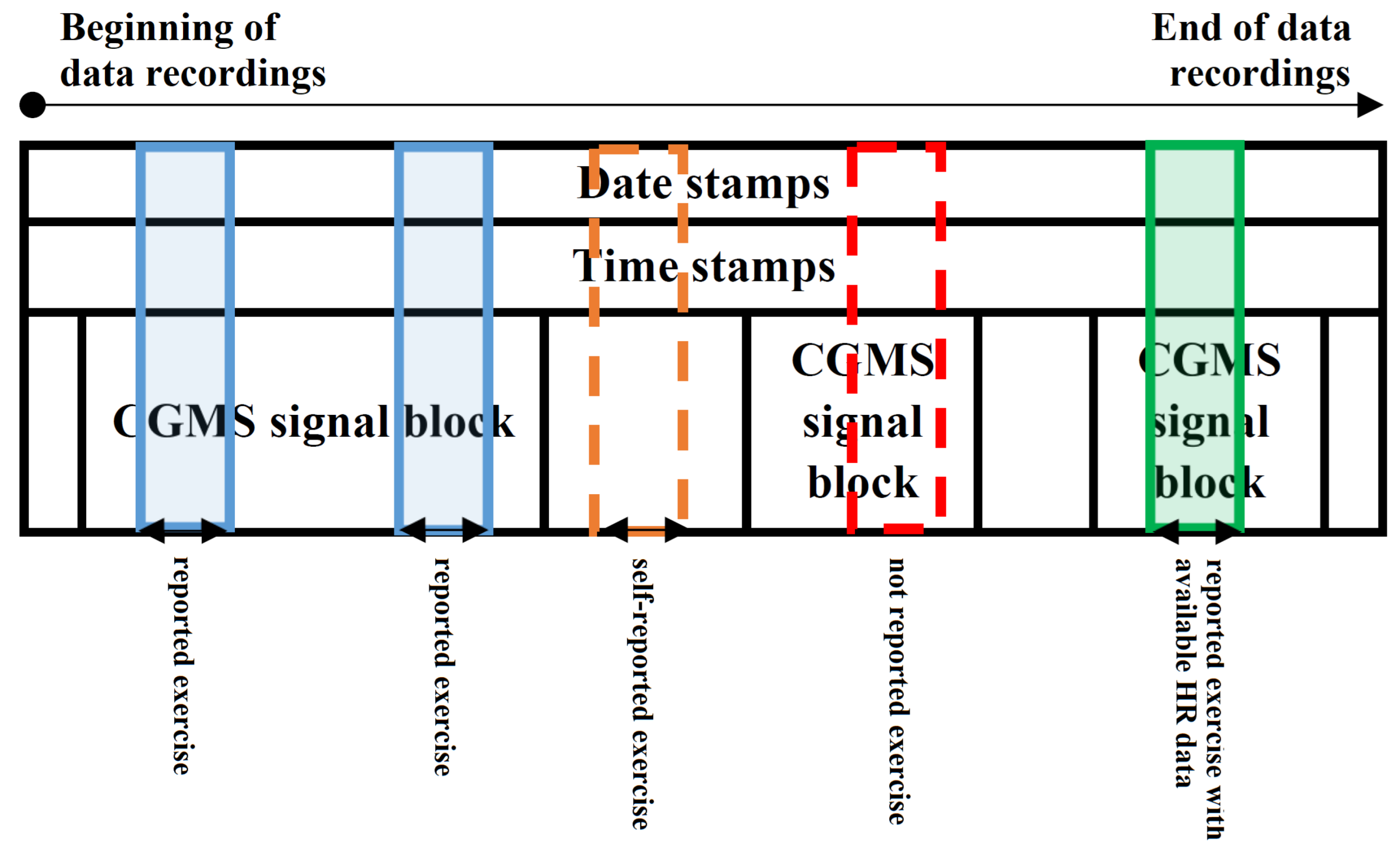
- CGM data in 24 h long blocks where self-reported exercise happened within the 24 h (e.g., Figure 1—blue and green regions). The exercise event was set to 1 where the exercise was ongoing. We made an exception—where the reported activity level was lower than 2, we set the exercise event to 0. The numerical properties of the extracted dataset can be seen in Table 1.
- (ii)
- CGM data in 24 h long blocks where self-reported exercise happened within the 24 h and HR data were also available (e.g., Figure 1—green region). The exercise event was set to 1 where the exercise was ongoing. We made an exception—where the reported activity level was lower than 2, the exercise event was set to 0. The numerical properties of the extracted dataset can be seen in Table 2.
2.3.2. The D1namo Dataset
2.4. Investigated Machine Learning Methods
- Logistic Regression (LR). The LR models provide the probability whether a given sample belongs to a particular class or not by using the logistic function: , where k is the steepness of the logistic curve, M is the maximum value of the curve, and is the inflection point [45]. During the training session, we allowed maximum 1000 iterations, and we applied -type penalty to measure the performance.
- AdaBoost Classifier (AdaBoost) represents a boosting technique used in machine learning as an ensemble method. The weights are re-assigned to each instance, with higher weights assigned to incorrectly classified instances. The purpose of boosting is to reduce bias and variances. It works on the principle of learners growing sequentially. Each subsequent learner is grown from previously grown learners except the first one. In simple words, weak learners are converted into strong ones [46]. Our model was set with maximum 50 trees.
- Decision Tree Classifier (DC) [47,48]. The DC is a flowchart kind of machine learning algorithm where each node represents a statistical probe on a given attribute. The branches are assigned to the possible outcomes of the probe while the leaf nodes represent a given class label. The paths from the roots to the leaves represent given classification rules. The goal of the DC is to learn rules by making predictions from features. Each branching point in the tree is a rule after which we obtain either the decision itself or a starting point of another subtree. The tree depth defines how many rules need to be applied step by step to obtain the result. In this given case, we did not limit the tree depth during training and all decisions were allowed to use any one of the features.
- Gaussian Naive Bayes (Gaussian) [49] is a very simple machine learning algorithm (also referred to as probabilistic classifier which is based on Bayes’ theorem). In general, the naive Bayes classifiers are highly scalable models, requiring a number of parameters linear in the number of variables in a given learning problem. When dealing with continuous or close-to-continuous data, a typical assumption is that the continuous values are associated with each class that are distributed according to a normal distribution.
- K-Nearest Neighbors Classifier (KNN) [50,51]. This method relies on labels and makes an approximation function for new data. The KNN algorithm assumes that the similar features “fall” close to each other (in numerical sense). The data are represented in a hyperspace based on the characteristics of the data. When new data arrive, the algorithm looks at the k-nearest neighbors at the decision. The prediction result is the class that received the most votes based on its neighbors. We use the tree implementation [52] of KNN with .
- Support Vector Machines [53]. This machine learning algorithm can be used for classification, regression, and also for outlier detection (anomaly detection). It is very efficient in high-dimensional spaces and also good when the number of dimensions (features) is greater than the sample number. It is very versatile in the case of using kernels. Common kernels are provided, but we can specify own kernels if we want. The main goal of the algorithm is to find a hyperplane in N-dimensional feature space. To separate classes, we can find many different hyperplanes, but the SVM finds the hyperplane which provides the maximum margin. We examined SVMs with 1000 iterations in five kernel variants: radial basis function kernel (SVM kernel = rbf), sigmoid kernel (SVM kernel = sigmoid), 3rd-degree polynomial kernel (SVM kernel = poly degree = 3), 5th-degree polynomial kernel (SVM kernel = poly degree = 5), and 10th-degree polynomial kernel (SVM kernel = poly degree = 10).
- Random Forest [54,55]. The Random Forest is based on decision trees: it creates different trees via training on different random sets of feature vectors from the training set that was selected according to the same rule. In prediction, each tree gives a rating, a vote, which is aggregated to provide a final decision according to the majority of the votes. These votes are aggregated. In our test, the Random Forest was built with 100 trees.
- Multi-Layer Perceptron Networks (MLP) [56,57]. A neuron consists of an input part, which is a vector, the weights of the neuron, which is also a vector, an activation function through which we pass the product of the input vector, and the transposition of the weighting vector. The last element of the neuron is the output, which is the value of the activation function. Activation function can be sigmoid, tangent hyperbolic, Gaussian function, etc. An MLP is realized when multiple neurons are organized next to each other—that is the so-called layer—and multiple layers of neurons are arranged in a row that aggregate the input in a complex way to realize the output of the MLP. The output is obtained by going through the network, layer by layer. The activation function is calculated for each neuron in each layer. In the end, the neuron with the highest value will be the output for that input, i.e., which neuron showed the highest activation for that input.All MLP models involved in this work used four hidden layers of sizes 100, 150, 100, and 50, respectively. They were all trained for maximum 1000 iterations. The deployed MLP models differ in their activation functions, which can be logistic, ReLU, or tanh.
2.5. Definition of Use-Cases for Model Development
- Recognizing physical activity based only on CGM signal using the cleaned data from the Ohio T1DM dataset (Table 1). Feature vector consists of BG sample points. Data structure: [Date stamp, Time stamp, BG level from CGM (concentration), Exercise (0/1)]. Of the dataset, 75% was used for training, the remaining 25% for testing.
- Recognizing physical activity based only on CGM signal using the cleaned data from the D1namo dataset. Feature vector consists of BG sample points. Data structure: [Date stamp, Time stamp, BG level from CGM (concentration), Exercise (0/1)]. Of the dataset, 75% was used for training, the remaining 25% for testing.
- Recognizing physical activity based on CGM and HR signals using the cleaned data from the Ohio T1DM dataset (Table 2). Feature vector consists of BG and HR sample points. Data structure: [Date stamp, Time stamp, BG level from CGM (concentration), HR level (integer), Exercise (0/1)]. Of the dataset, 75% was used for training, the remaining 25% for testing.
- Recognizing physical activity based on CGM and HR signals using the cleaned data from the D1namo dataset. Feature vector consists of BG and HR sample points. Data structure: [Date stamp, Time stamp, BG level from CGM (concentration), HR level (integer), Exercise (0/1)]. Of the dataset, 75% was used for training, the remaining 25% for testing.
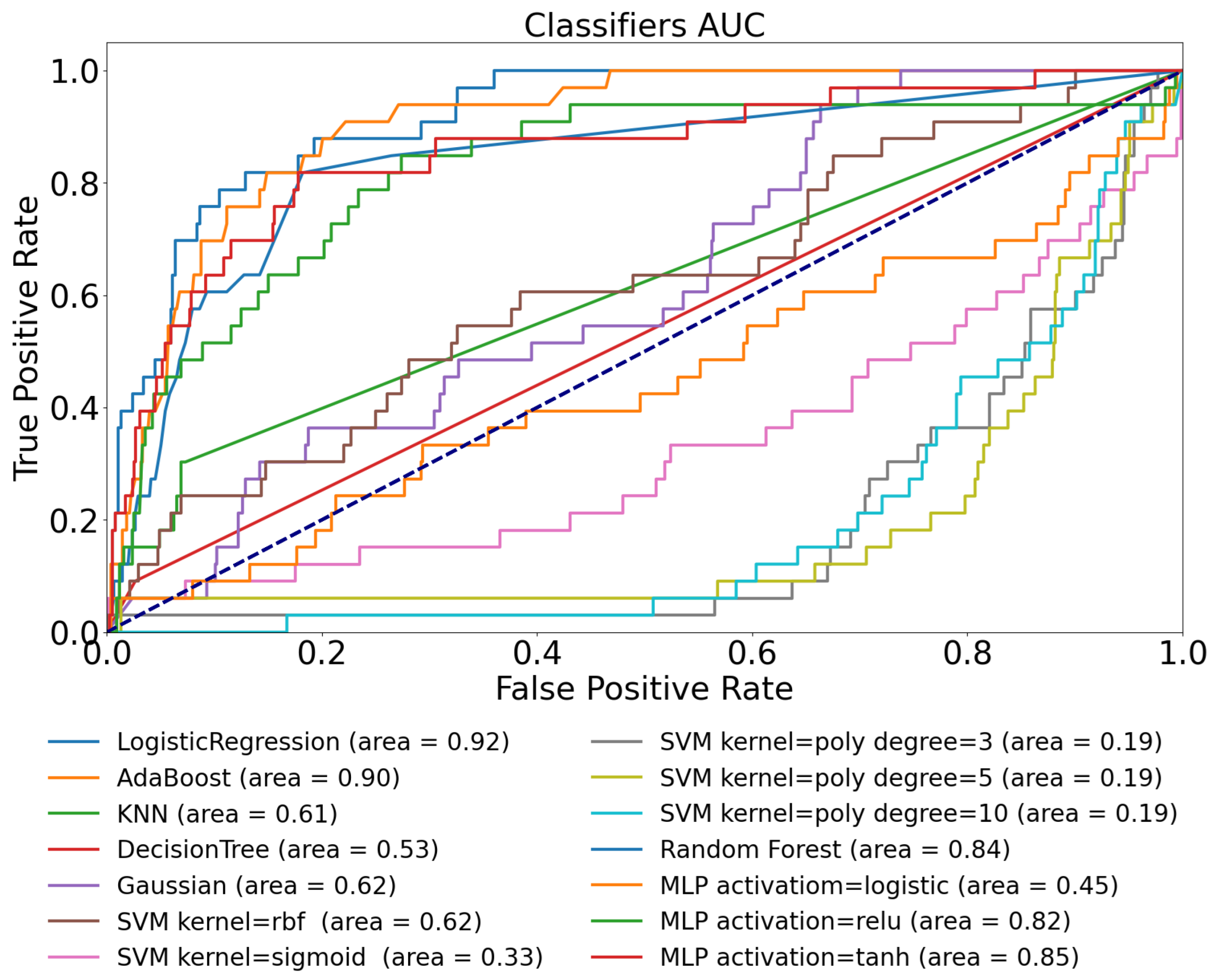
- Recognizing physical activity based on CGM and HR signals using the cleaned data from the Ohio T1DM (Table 2) and D1namo datasets. Feature vector consists of BG sample points. Data structure: [Date stamp, Time stamp, BG level from CGM (concentration), HR level (integer), Exercise (0/1)]. The train data were the Ohio T1DM data records while the test data were the D1namo data records. All records of the Ohio T1DM dataset were used for training, and all records of D1namo dataset for testing.This use-case can be applied to strengthen our hypothesis as to whether there are many non-reported physical activities in the original Ohio T1DM dataset (where CGM signal was available, physical activity was not reported; however, physical activity possibly happened). Furthermore, this use-case can be applied for data annotation as well on the original Ohio T1DM dataset to select the presumable non-reported physical activities.
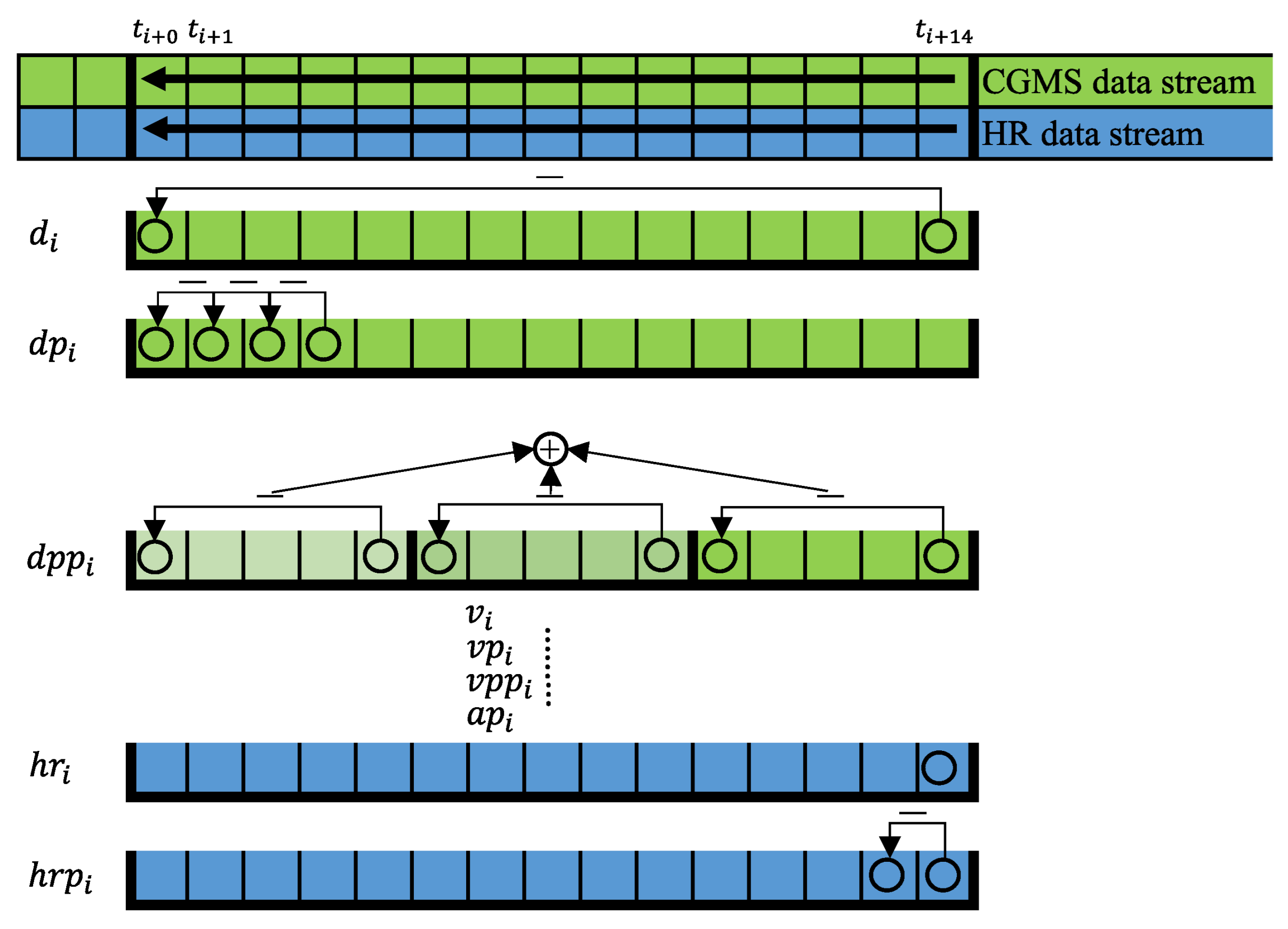
2.6. Feature Extraction
- The end-to-end difference in the blood glucose level (d) in the window.
- The blood glucose level difference between two consecutive sampled points within the window ()
- The change in the blood glucose levels in the three mini windows, from beginning to end ()
- End-to-end blood glucose level change speed (v):
- The blood glucose level change speed between two consecutive sampled points ()
- The blood glucose level change speed in all mini sliding window measured points. From beginning to end ()
- The acceleration of blood glucose level change speed among three consecutive sampled points ()
- The HR measured at the CGM sample time (),
- The end-to-end heart rate difference, the difference between the first heart rate measured point and the last heart rate measured point, which point is between two consecutive glucose sample times (),
2.7. Performance Metrics
- Accuracy () represents the rate of correct decisions, defined as
- Recall, also known as sensitivity or true-positive rate (), is defined as
- Specificity, also known as true-negative rate (), is defined as
- Precision, also known as positive prediction value (), is defined as
- False-positive rate () is defined as
- -score (), also known as Dice score, is defined as
3. Results
3.1. Ohio T1DM Dataset Using Only Blood Glucose Level Features—Use-Case 1
3.2. D1namo Dataset Using Blood Glucose Level Features Only—Use-Case 2
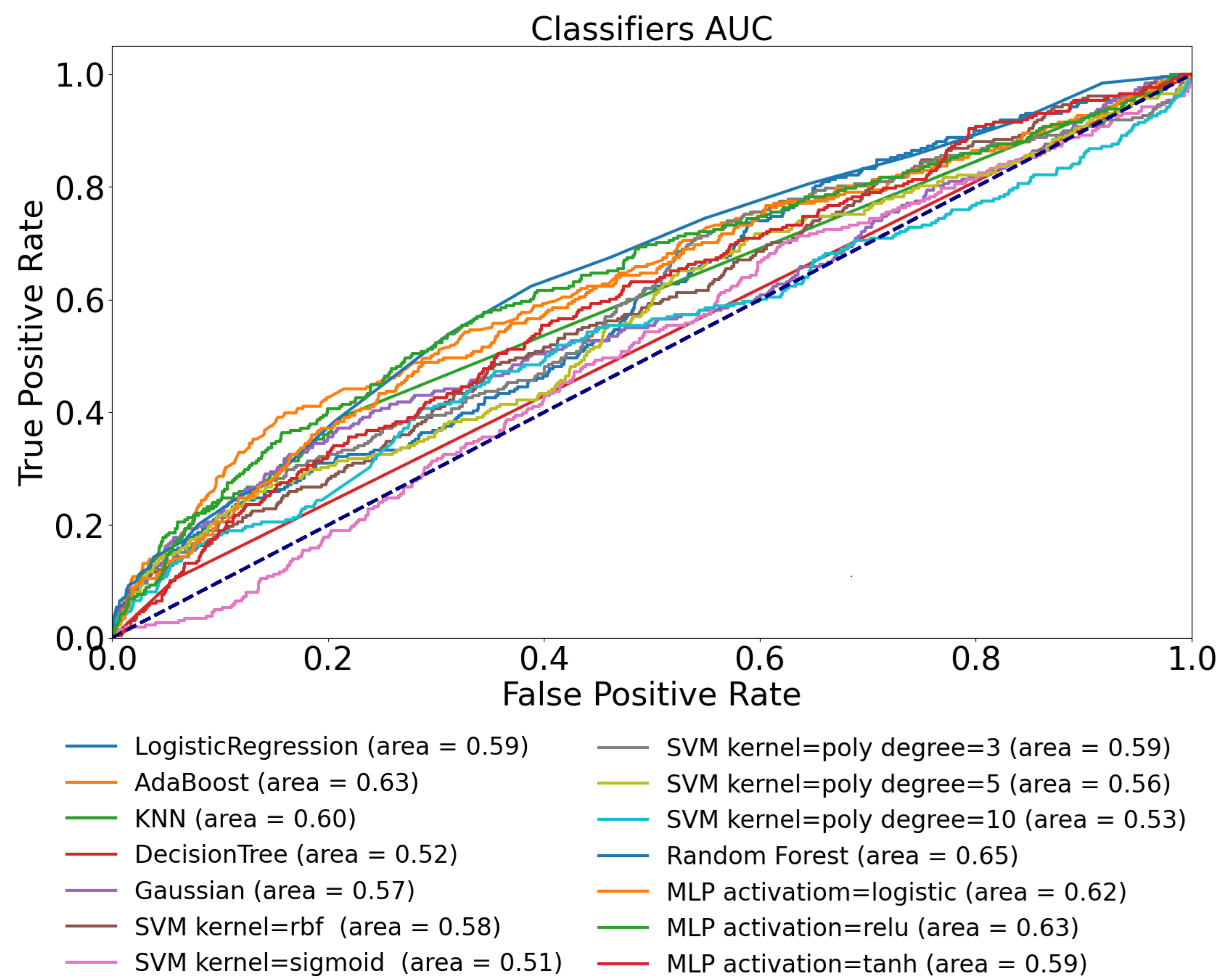
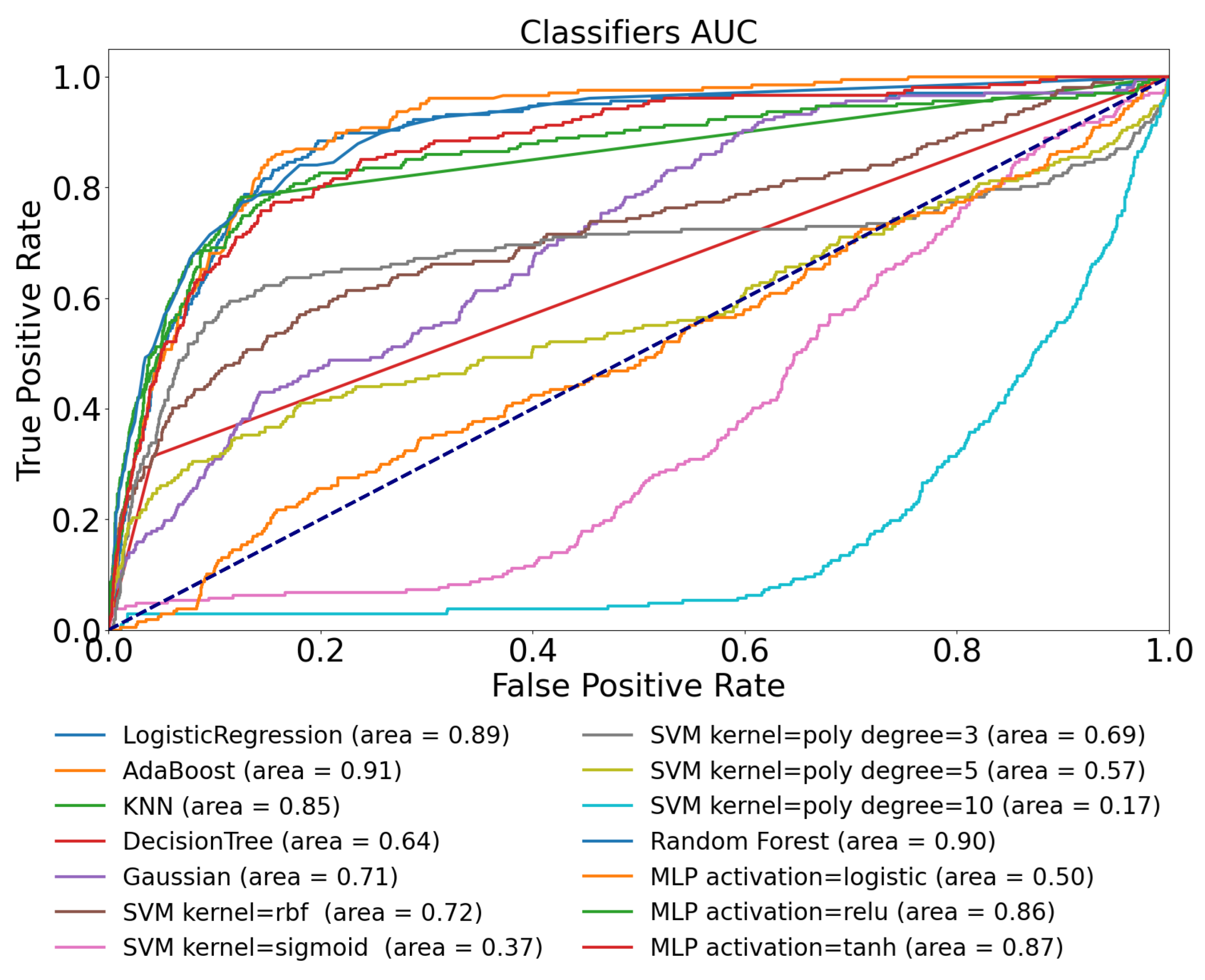
3.3. Ohio T1DM Dataset with Blood Glucose and Heart Rate Features—Use-Case 3
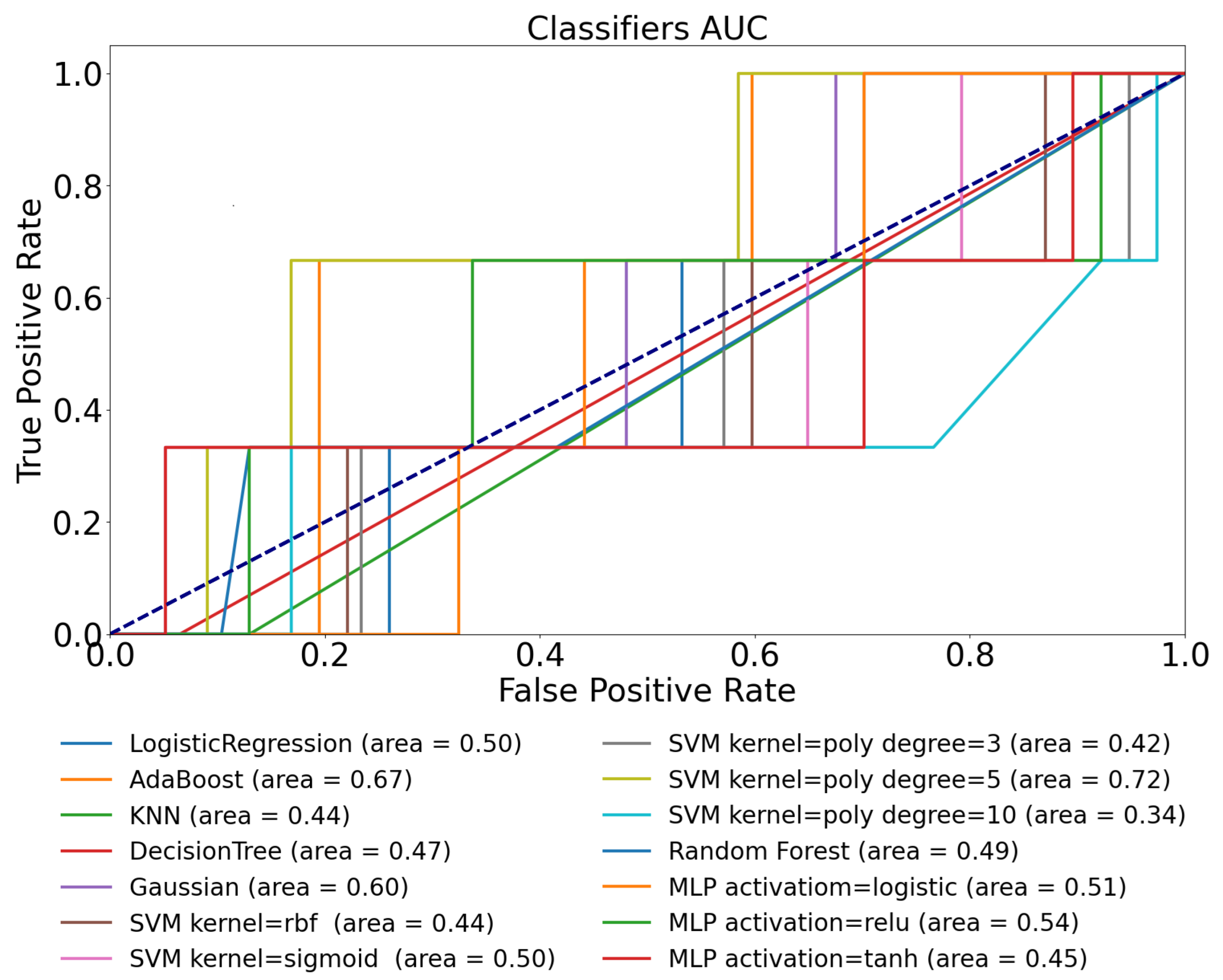
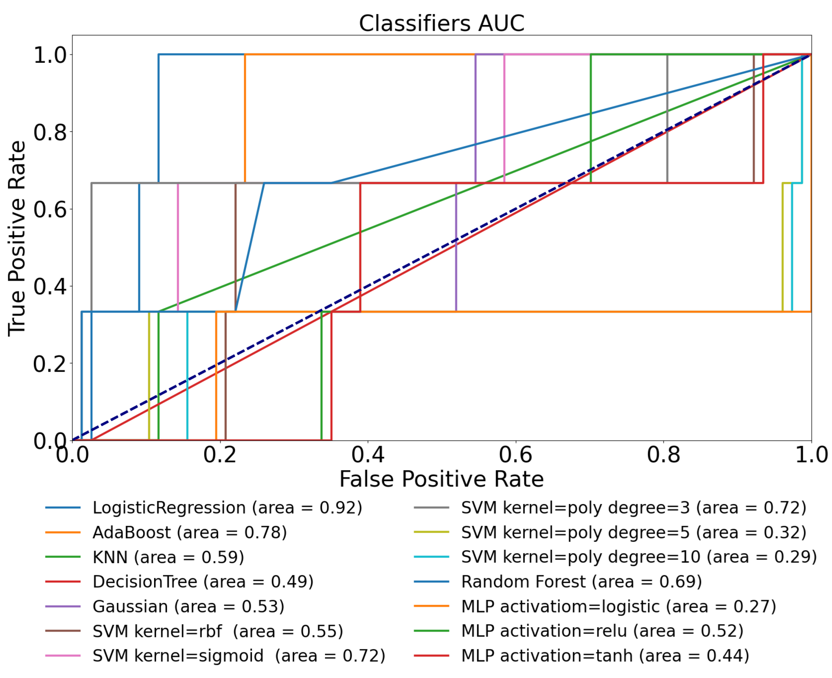
3.4. D1namo Dataset with Blood Glucose and Heart Rate Features—Use-Case 4
3.5. Experiences with Use-Case 5
4. Discussion
5. Conclusions
Author Contributions
Funding
Institutional Review Board Statement
Informed Consent Statement
Data Availability Statement
Conflicts of Interest
Ethical Statement
Abbreviations
| ACC | Accuracy |
| AdaBoost | AdaBoost Classifier |
| AUC | Area Under the Curve |
| BG | Blood Glucose |
| BGL | Blood Glucose Level |
| BGV | Blood Glucose Variability |
| CAN | Cardiac Autonomic Neuropathy |
| CGM | Continuous Glucose Monitoring System |
| DM | Diabetes Mellitus |
| DTC | Decision Tree Classifier |
| F | F score |
| FN | False Negative |
| FP | False Positive |
| FPR | False-Positive Rate |
| Gaussian | Gaussian Naive Bayes |
| HR | Heart Rate |
| HRV | Heart Rate Variability |
| IMU | Inertia Measurement Unit |
| KNN | K-Nearest Neighbors Classifier |
| LR | Logistic Regression |
| LSTM | Long short-term memory |
| MLP | Multi-Layer Perceptron Networks |
| PPV | Positive Prediction Value—Precision |
| RF | Random Forest |
| ROC | Receiver Operating Characteristic |
| SVM | Support Vector Machines |
| T1DM | Type 1 Diabetes Mellitus |
| T2DM | Type 2 Diabetes Mellitus |
| TN | True Negative |
| TNR | True-Negative Rate—Specificity |
| TP | True Positive |
| TPR | True-Positive Rate—Recall |
References
- Deng, D.; Yan, N. GLUT, SGLT, and SWEET: Structural and mechanistic investigations of the glucose transporters. Protein Sci. 2016, 25, 546–558. [Google Scholar] [CrossRef] [PubMed] [Green Version]
- Holt, R.I.; Cockram, C.; Flyvbjerg, A.; Goldstein, B.J. Textbook of Diabetes; John Wiley & Sons: Chichester, UK, 2017. [Google Scholar]
- Bird, S.R.; Hawley, J.A. Update on the effects of physical activity on insulin sensitivity in humans. BMJ Open Sport Exerc. Med. 2017, 2, e000143. [Google Scholar] [CrossRef] [PubMed] [Green Version]
- Zhao, C.; Yang, C.F.; Tang, S.; Wai, C.; Zhang, Y.; Portillo, M.P.; Paoli, P.; Wu, Y.J.; Cheang, W.S.; Liu, B.; et al. Regulation of glucose metabolism by bioactive phytochemicals for the management of type 2 diabetes mellitus. Crit. Rev. Food Sci. Nutr. 2019, 59, 830–847. [Google Scholar] [CrossRef]
- Richter, E.A.; Hargreaves, M. Exercise, GLUT4, and skeletal muscle glucose uptake. Physiol. Rev. 2013. [Google Scholar] [CrossRef] [PubMed] [Green Version]
- Sylow, L.; Kleinert, M.; Richter, E.A.; Jensen, T.E. Exercise-stimulated glucose uptake—Regulation and implications for glycaemic control. Nat. Rev. Endocrinol. 2017, 13, 133–148. [Google Scholar] [CrossRef]
- Colberg, S.R.; Sigal, R.J.; Yardley, J.E.; Riddell, M.C.; Dunstan, D.W.; Dempsey, P.C.; Horton, E.S.; Castorino, K.; Tate, D.F. Physical Activity/Exercise and Diabetes: A Position Statement of the American Diabetes Association. Diabetes Care 2016, 39, 2065–2079. [Google Scholar] [CrossRef] [Green Version]
- American Diabetes Association. 5. Lifestyle management: Standards of medical care in diabetes—2019. Diabetes Care 2019, 42, S46–S60. [Google Scholar] [CrossRef] [Green Version]
- Martyn-Nemeth, P.; Quinn, L.; Penckofer, S.; Park, C.; Hofer, V.; Burke, L. Fear of hypoglycemia: Influence on glycemic variability and self-management behavior in young adults with type 1 diabetes. J. Diabetes Its Complicat. 2017, 31, 735–741. [Google Scholar] [CrossRef] [Green Version]
- Jeandidier, N.; Riveline, J.P.; Tubiana-Rufi, N.; Vambergue, A.; Catargi, B.; Melki, V.; Charpentier, G.; Guerci, B. Treatment of diabetes mellitus using an external insulin pump in clinical practice. Diabetes Metab. 2008, 34, 425–438. [Google Scholar] [CrossRef]
- Adams, P.O. The impact of brief high-intensity exercise on blood glucose levels. Diabetes Metab. Syndr. Obes. 2013, 6, 113–122. [Google Scholar] [CrossRef]
- Stavdahl, Ø.; Fougner, A.L.; Kölle, K.; Christiansen, S.C.; Ellingsen, R.; Carlsen, S.M. The artificial pancreas: A dynamic challenge. IFAC-PapersOnLine 2016, 49, 765–772. [Google Scholar] [CrossRef]
- Tagougui, S.; Taleb, N.; Molvau, J.; Nguyen, É.; Raffray, M.; Rabasa-Lhoret, R. Artificial pancreas systems and physical activity in patients with type 1 diabetes: Challenges, adopted approaches, and future perspectives. J. Diabetes Sci. Technol. 2019, 13, 1077–1090. [Google Scholar] [CrossRef] [PubMed]
- Ekelund, U.; Poortvliet, E.; Yngve, A.; Hurtig-Wennlöv, A.; Nilsson, A.; Sjöström, M. Heart rate as an indicator of the intensity of physical activity in human adolescents. Eur. J. Appl. Physiol. 2001, 85, 244–249. [Google Scholar] [CrossRef]
- Crema, C.; Depari, A.; Flammini, A.; Sisinni, E.; Haslwanter, T.; Salzmann, S. IMU-based solution for automatic detection and classification of exercises in the fitness scenario. In Proceedings of the 2017 IEEE Sensors Applications Symposium (SAS), Glassboro, NJ, USA, 13–15 March 2017; pp. 1–6. [Google Scholar] [CrossRef]
- Allahbakhshi, H.; Hinrichs, T.; Huang, H.; Weibel, R. The key factors in physical activity type detection using real-life data: A systematic review. Front. Physiol. 2019, 10, 75. [Google Scholar] [CrossRef] [Green Version]
- Cescon, M.; Choudhary, D.; Pinsker, J.E.; Dadlani, V.; Church, M.M.; Kudva, Y.C.; Doyle, F.J., III; Dassau, E. Activity detection and classification from wristband accelerometer data collected on people with type 1 diabetes in free-living conditions. Comput. Biol. Med. 2021, 135, 104633. [Google Scholar] [CrossRef] [PubMed]
- Verrotti, A.; Prezioso, G.; Scattoni, R.; Chiarelli, F. Autonomic neuropathy in diabetes mellitus. Front. Endocrinol. 2014, 5, 205. [Google Scholar] [CrossRef] [PubMed] [Green Version]
- Agashe, S.; Petak, S. Cardiac autonomic neuropathy in diabetes mellitus. Methodist Debakey Cardiovasc. J. 2018, 14, 251. [Google Scholar] [CrossRef]
- Helleputte, S.; De Backer, T.; Lapauw, B.; Shadid, S.; Celie, B.; Van Eetvelde, B.; Vanden Wyngaert, K.; Calders, P. The relationship between glycaemic variability and cardiovascular autonomic dysfunction in patients with type 1 diabetes: A systematic review. Diabetes/Metabolism Res. Rev. 2020, 36, e3301. [Google Scholar] [CrossRef] [Green Version]
- Vijayan, V.; Connolly, J.P.; Condell, J.; McKelvey, N.; Gardiner, P. Review of Wearable Devices and Data Collection Considerations for Connected Health. Sensors 2021, 21, 5589. [Google Scholar] [CrossRef]
- McCarthy, C.; Pradhan, N.; Redpath, C.; Adler, A. Validation of the Empatica E4 wristband. In Proceedings of the 2016 IEEE EMBS International Student Conference (ISC), Ottawa, ON, Canada, 29–31 May 2016; pp. 1–4. [Google Scholar] [CrossRef]
- Liang, L.; Kong, F.W.; Martin, C.; Pham, T.; Wang, Q.; Duncan, J.; Sun, W. Machine learning–based 3-D geometry reconstruction and modeling of aortic valve deformation using 3-D computed tomography images. Int. J. Numer. Methods Biomed. Eng. 2017, 33, e2827. [Google Scholar] [CrossRef] [PubMed] [Green Version]
- Lundberg, S.M.; Nair, B.; Vavilala, M.S.; Horibe, M.; Eisses, M.J.; Adams, T.; Liston, D.E.; Low, D.K.W.; Newman, S.F.; Kim, J.; et al. Explainable machine-learning predictions for the prevention of hypoxaemia during surgery. Nat. Biomed. Eng. 2018, 2, 749–760. [Google Scholar] [CrossRef] [PubMed]
- Ostrogonac, S.; Pakoci, E.; Sečujski, M.; Mišković, D. Morphology-based vs unsupervised word clustering for training language models for Serbian. Acta Polytech. Hung. 2019, 16, 183–197. [Google Scholar] [CrossRef]
- Machová, K.; Mach, M.; Hrešková, M. Classification of Special Web Reviewers Based on Various Regression Methods. Acta Polytech. Hung. 2020, 17, 229–248. [Google Scholar] [CrossRef]
- Hayeri, A. Predicting Future Glucose Fluctuations Using Machine Learning and Wearable Sensor Data. Diabetes 2018, 67, A193. [Google Scholar] [CrossRef]
- Daskalaki, E.; Diem, P.; Mougiakakou, S.G. Model-free machine learning in biomedicine: Feasibility study in type 1 diabetes. PLoS ONE 2016, 11, e0158722. [Google Scholar] [CrossRef] [PubMed] [Green Version]
- Woldaregay, A.Z.; Årsand, E.; Botsis, T.; Albers, D.; Mamykina, L.; Hartvigsen, G. Data-Driven Blood Glucose Pattern Classification and Anomalies Detection: Machine-Learning Applications in Type 1 Diabetes. J. Med. Internet Res. 2019, 21, e11030. [Google Scholar] [CrossRef] [PubMed] [Green Version]
- Contreras, I.; Vehi, J. Artificial intelligence for diabetes management and decision support: Literature review. J. Med. Internet Res. 2018, 20, e10775. [Google Scholar] [CrossRef] [PubMed]
- Dénes-Fazakas, L.; Szilágyi, L.; Tasic, J.; Kovács, L.; Eigner, G. Detection of physical activity using machine learning methods. In Proceedings of the 2020 IEEE 20th International Symposium on Computational Intelligence and Informatics (CINTI), Budapest, Hungary, 5–7 November 2020; pp. 167–172. [Google Scholar] [CrossRef]
- TensorFlow Core v2.4.0. Available online: https://www.tensorflow.org/api_docs (accessed on 27 October 2022).
- Scikit-Learn User Guide. Available online: https://scikit-learn.org/0.18/_downloads/scikit-learn-docs.pdf (accessed on 27 October 2022).
- NumPy Documentation. Available online: https://numpy.org/doc/ (accessed on 27 October 2022).
- Pandas Documentation. Available online: https://pandas.pydata.org/docs/ (accessed on 27 October 2022).
- Jupyter Notebook Documentation. Available online: https://readthedocs.org/projects/jupyter-notebook/downloads/pdf/latest/ (accessed on 27 October 2022).
- Colaboratory. Available online: https://research.google.com/colaboratory/faq.html (accessed on 27 October 2022).
- Marling, C.; Bunescu, R.C. The Ohio T1DM dataset for blood glucose level prediction. In Proceedings of the KHD@ IJCAI, Stockholm, Schweden, 13 July 2018. [Google Scholar]
- Farri, O.; Guo, A.; Hasan, S.; Ibrahim, Z.; Marling, C.; Raffa, J.; Rubin, J.; Wu, H. Blood Glucose Prediction Challenge. In Proceedings of the 3rd International Workshop on Knowledge Discovery in Healthcare Data, CEUR Workshop Proceedings (CEUR-WS.org), Stockholm, Sweden, 13 July 2018. [Google Scholar]
- Bach, K.; Bunescu, R.C.; Marling, C.; Wiratunga, N. Blood Glucose Prediction Challenge. In Proceedings of the the 5th International Workshop on Knowledge Discovery in Healthcare Data, 24th European Conference on Artificial Intelligence (ECAI 2020), Santiago de Compostela, Spain & Virtually, 29–30 August 2020. [Google Scholar]
- Marling, C.; Bunescu, R. The ohiot1dm dataset for blood glucose level prediction: Update 2020. KHD@ IJCAI 2020, 2675, 71. [Google Scholar]
- Dubosson, F.; Ranvier, J.E.; Bromuri, S.; Calbimonte, J.P.; Ruiz, J.; Schumacher, M. The open D1NAMO dataset: A multi-modal dataset for research on non-invasive type 1 diabetes management. Inform. Med. Unlocked 2018, 13, 92–100. [Google Scholar] [CrossRef]
- Zephyr Bioharness 3.0 User Manual. 2012. Available online: https://www.zephyranywhere.com/media/download/bioharness3-user-manual.pdf (accessed on 27 October 2022).
- Pedregosa, F.; Varoquaux, G.; Gramfort, A.; Michel, V.; Thirion, B.; Grisel, O.; Blondel, M.; Prettenhofer, P.; Weiss, R.; Dubourg, V.; et al. Scikit-learn: Machine Learning in Python. J. Mach. Learn. Res. 2011, 12, 2825–2830. [Google Scholar]
- Cox, D.R. The regression analysis of binary sequences (with discussion). J. R. Stat. Soc. B 1958, 20, 215–242. [Google Scholar]
- Freund, Y.; Schapire, R.E. Experiments with a new boosting algorithm. In Proceedings of the 13th International Conference on Machine Learning, Bari, Italy, 3–6 July 1996; pp. 148–157. [Google Scholar]
- Akers, S.B. Binary decision diagrams. IEEE Trans. Comput. 1978, C-27, 509–516. [Google Scholar] [CrossRef]
- Szilágyi, L.; Iclănzan, D.; Kapás, Z.; Szabó, Z.; Győrfi, Á.; Lefkovits, L. Low and high grade glioma segmentation in multispectral brain MRI data. Acta Univ.-Sapientiae Inform. 2018, 10, 110–132. [Google Scholar] [CrossRef] [Green Version]
- Chow, C.K. An optimum character recognition system using decision functions. IRE Trans. Comput. 1957, EC-6, 247–254. [Google Scholar] [CrossRef]
- Cover, T.M.; Hart, P.E. Nearest neighbor pattern classification. IEEE Trans. Inf. Theory 1967, IT-13, 21–27. [Google Scholar] [CrossRef] [Green Version]
- Goodfellow, I.; Bengio, Y.; Courville, A. Deep Learning; MIT Press: Cambridge, MA, USA, 2016; Available online: http://www.deeplearningbook.org (accessed on 27 October 2022).
- Bentley, J.L. Multidimensional binary search trees used for associative searching. Commun. ACM 1975, 18, 509–517. [Google Scholar] [CrossRef]
- Cortes, C.; Vapnik, V. Support-vector networks. Mach. Learn. 1995, 20, 273–297. [Google Scholar] [CrossRef]
- Breiman, L. Random forests. Mach. Learn. 2001, 45, 5–32. [Google Scholar] [CrossRef] [Green Version]
- Alfaro-Cortés, E.; Alfaro-Navarro, J.L.; Gámez, M.; García, N. Using random forest to interpret out-of-control signals. Acta Polytech. Hung. 2020, 17, 115–130. [Google Scholar] [CrossRef]
- Rumelhart, D.E.; Hinton, G.E.; Williams, R.J. Learning representations by back-propagating errors. Nature 1986, 323, 533–536. [Google Scholar] [CrossRef]
- Alvarez, K.; Urenda, J.; Csiszár, O.; Csiszár, G.; Dombi, J.; Eigner, G.; Kreinovich, V. Towards Fast and Understandable Computations: Which “And”-and “Or”-Operations Can Be Represented by the Fastest (ie, 1-Layer) Neural Networks? Which Activations Functions Allow Such Representations? Dep. Tech. Rep. (CS) 2020, 1443. [Google Scholar] [CrossRef]
- Liu, Y.; Wang, Y.; Qi, H.; Ju, X. SuperPruner: Automatic Neural Network Pruning via Super Network. Sci. Program. 2021, 2021, 9971669. [Google Scholar] [CrossRef]
- Koctúrová, M.; Juhár, J. EEG-based Speech Activity Detection. Acta Polytech. Hung. 2021, 18, 65–77. [Google Scholar]
- Géron, A. Hands-On Machine Learning with Scikit-Learn, Keras, and TensorFlow: Concepts, Tools, and Techniques to Build Intelligent Systems; O’Reilly Media: Newton, MA, USA, 2019. [Google Scholar]
- Askari, M.R.; Rashid, M.; Sun, X.; Sevil, M.; Shahidehpour, A.; Kawaji, K.; Cinar, A. Meal and Physical Activity Detection from Free-Living Data for Discovering Disturbance Patterns of Glucose Levels in People with Diabetes. BioMedInformatics 2022, 2, 297–317. [Google Scholar] [CrossRef]
- Tyler, N.S.; Mosquera-Lopez, C.; Young, G.M.; El Youssef, J.; Castle, J.R.; Jacobs, P.G. Quantifying the impact of physical activity on future glucose trends using machine learning. iScience 2022, 25, 103888. [Google Scholar] [CrossRef] [PubMed]
- Contador, S.; Colmenar, J.M.; Garnica, O.; Velasco, J.M.; Hidalgo, J.I. Blood glucose prediction using multi-objective grammatical evolution: Analysis of the “agnostic” and “what-if” scenarios. Genet. Program. Evolvable Mach. 2022, 23, 161–192. [Google Scholar] [CrossRef]
- Kushner, T.; Breton, M.D.; Sankaranarayanan, S. Multi-Hour Blood Glucose Prediction in Type 1 Diabetes: A Patient-Specific Approach Using Shallow Neural Network Models. Diabetes Technol. Ther. 2020, 22, 883–891. [Google Scholar] [CrossRef]


| Ohio T1DM Patient (OP) ID | Number of Records | Total Time Duration in Days |
|---|---|---|
| OP3 | 546 | 2 |
| OP8 | 2730 | 10 |
| OP9 | 546 | 2 |
| OP10 | 3276 | 12 |
| OP14 | 2730 | 10 |
| OP18 | 546 | 2 |
| OP19 | 7917 | 29 |
| OP20 | 819 | 3 |
| OP21 | 1638 | 6 |
| OP22 | 1365 | 5 |
| OP23 | 4914 | 18 |
| Total | 27,027 | 99 |
| Ohio T1DM Patient (OP) ID | Number of Records | Total Time Duration in Days |
|---|---|---|
| OP8 | 2730 | 10 |
| OP9 | 546 | 2 |
| OP10 | 3276 | 12 |
| OP14 | 2730 | 10 |
| OP18 | 546 | 2 |
| OP19 | 7917 | 29 |
| OP20 | 819 | 3 |
| OP21 | 1638 | 6 |
| Total | 20,202 | 74 |
| D1namo Patient | Record Count for CGM Features | Record Count for CGM and HR Features | Total Time Duration in Days |
|---|---|---|---|
| Patient 1 | 939 | 858 | 6 |
| Patient 2 | 1575 | 1440 | 5 |
| Patient 3 | 185 | 166 | 2 |
| Patient 4 | 1383 | 1266 | 4 |
| Patient 5 | 1375 | 1251 | 4 |
| Patient 6 | 1225 | 1108 | 6 |
| Patient 7 | 966 | 879 | 5 |
| Patient 8 | 1189 | 1088 | 5 |
| Patient 9 | 135 | 85 | 2 |
| Total | 8972 | 8141 | 39 |
| Classifier | ACC | TPR | TNR | PPV | F1 |
|---|---|---|---|---|---|
| Logistic Regression | 0.566 | 0.487 | 0.645 | 0.578 | 0.555 |
| AdaBoost | 0.634 | 0.602 | 0.666 | 0.643 | 0.632 |
| KNN | 0.598 | 0.411 | 0.784 | 0.656 | 0.539 |
| Decision Tree | 0.527 | 0.114 | 0.940 | 0.657 | 0.204 |
| Gaussian | 0.602 | 0.496 | 0.708 | 0.629 | 0.583 |
| SVM kernel = rbf | 0.514 | 0.462 | 0.566 | 0.515 | 0.509 |
| SVM kernel = sigmoid | 0.506 | 0.500 | 0.512 | 0.506 | 0.506 |
| SVM kernel = poly, deg = 3 | 0.536 | 0.581 | 0.492 | 0.533 | 0.532 |
| SVM kernel = poly, deg = 5 | 0.509 | 0.547 | 0.471 | 0.508 | 0.506 |
| SVM kernel = poly, deg = 10 | 0.487 | 0.377 | 0.597 | 0.483 | 0.462 |
| Random Forest | 0.611 | 0.602 | 0.619 | 0.612 | 0.610 |
| MLP activation = logistic | 0.609 | 0.589 | 0.629 | 0.614 | 0.608 |
| MLP activation = ReLU | 0.610 | 0.547 | 0.674 | 0.626 | 0.604 |
| MLP activation = tanh | 0.579 | 0.593 | 0.566 | 0.577 | 0.579 |
| Classifier | ACC | TPR | TNR | PPV | F1 |
|---|---|---|---|---|---|
| Logistic Regression | 0.606 | 0.667 | 0.546 | 0.595 | 0.600 |
| AdaBoost | 0.727 | 1.000 | 0.454 | 0.647 | 0.625 |
| KNN | 0.788 | 0.667 | 0.910 | 0.881 | 0.770 |
| Decision Tree | 0.494 | 0.000 | 0.988 | 0.000 | 0.000 |
| Gaussian | 0.669 | 1.000 | 0.337 | 0.602 | 0.504 |
| SVM kernel = rbf | 0.669 | 1.000 | 0.337 | 0.602 | 0.504 |
| SVM kernel = sigmoid | 0.403 | 0.000 | 0.806 | 0.000 | 0.000 |
| SVM kernel = poly, deg = 3 | 0.537 | 0.333 | 0.741 | 0.563 | 0.460 |
| SVM kernel = poly, deg = 5 | 0.805 | 1.000 | 0.611 | 0.720 | 0.758 |
| SVM kernel = poly, deg = 10 | 0.602 | 0.333 | 0.871 | 0.721 | 0.482 |
| Random Forest | 0.708 | 1.000 | 0.415 | 0.631 | 0.587 |
| MLP activation = logistic | 0.606 | 0.667 | 0.546 | 0.595 | 0.600 |
| MLP activation = ReLU | 0.697 | 0.667 | 0.728 | 0.710 | 0.696 |
| MLP activation = tanh | 0.695 | 1.000 | 0.389 | 0.621 | 0.561 |
| Classifier | ACC | TPR | TNR | PPV | F1 |
|---|---|---|---|---|---|
| Logistic Regression | 0.832 | 0.850 | 0.814 | 0.820 | 0.831 |
| AdaBoost | 0.827 | 0.819 | 0.835 | 0.832 | 0.827 |
| KNN | 0.821 | 0.768 | 0.874 | 0.859 | 0.817 |
| Decision Tree | 0.615 | 0.275 | 0.954 | 0.857 | 0.427 |
| Gaussian | 0.632 | 0.544 | 0.720 | 0.660 | 0.619 |
| SVM kernel = rbf | 0.666 | 0.712 | 0.621 | 0.652 | 0.663 |
| SVM kernel = sigmoid | 0.621 | 0.664 | 0.578 | 0.611 | 0.618 |
| SVM kernel = poly, deg = 3 | 0.466 | 0.465 | 0.466 | 0.466 | 0.466 |
| SVM kernel = poly, deg = 5 | 0.287 | 0.435 | 0.138 | 0.336 | 0.210 |
| SVM kernel = poly, deg = 10 | 0.328 | 0.409 | 0.247 | 0.352 | 0.308 |
| Random Forest | 0.827 | 0.811 | 0.843 | 0.838 | 0.827 |
| MLP activation = logistic | 0.536 | 0.443 | 0.629 | 0.544 | 0.520 |
| MLP activation = ReLU | 0.779 | 0.768 | 0.791 | 0.786 | 0.779 |
| MLP activation = tanh | 0.807 | 0.789 | 0.825 | 0.818 | 0.806 |
| Classifier | ACC | TPR | TNR | PPV | F1 |
|---|---|---|---|---|---|
| Logistic Regression | 0.922 | 1.000 | 0.845 | 0.866 | 0.916 |
| AdaBoost | 0.792 | 1.000 | 0.585 | 0.707 | 0.738 |
| KNN | 0.801 | 0.667 | 0.936 | 0.912 | 0.779 |
| Decision Tree | 0.654 | 0.333 | 0.975 | 0.930 | 0.497 |
| Gaussian | 0.439 | 0.333 | 0.546 | 0.423 | 0.414 |
| SVM kernel = rbf | 0.511 | 0.333 | 0.689 | 0.517 | 0.449 |
| SVM kernel = sigmoid | 0.736 | 0.667 | 0.806 | 0.774 | 0.730 |
| SVM kernel = poly, deg = 3 | 0.814 | 0.667 | 0.962 | 0.946 | 0.788 |
| SVM kernel = poly, deg = 5 | 0.717 | 0.667 | 0.767 | 0.741 | 0.713 |
| SVM kernel = poly, deg = 10 | 0.743 | 0.667 | 0.819 | 0.786 | 0.735 |
| Random Forest | 0.945 | 1.000 | 0.889 | 0.901 | 0.941 |
| MLP activation = logistic | 0.593 | 0.667 | 0.520 | 0.581 | 0.584 |
| MLP activation = ReLU | 0.589 | 0.333 | 0.845 | 0.682 | 0.478 |
| MLP activation = tanh | 0.762 | 0.667 | 0.858 | 0.824 | 0.750 |
| Classifier | ACC | TPR | TNR | PPV | F1 |
|---|---|---|---|---|---|
| Logistic Regression | 0.845 | 0.818 | 0.871 | 0.864 | 0.844 |
| AdaBoost | 0.844 | 0.909 | 0.778 | 0.804 | 0.838 |
| KNN | 0.617 | 0.303 | 0.931 | 0.814 | 0.457 |
| Decision Tree | 0.522 | 0.061 | 0.983 | 0.778 | 0.114 |
| Gaussian | 0.579 | 0.485 | 0.673 | 0.597 | 0.564 |
| SVM kernel = rbf | 0.611 | 0.606 | 0.616 | 0.612 | 0.611 |
| SVM kernel = sigmoid | 0.649 | 0.606 | 0.693 | 0.664 | 0.647 |
| SVM kernel = poly, deg = 3 | 0.299 | 0.364 | 0.234 | 0.322 | 0.285 |
| SVM kernel = poly, deg = 5 | 0.391 | 0.667 | 0.114 | 0.429 | 0.195 |
| SVM kernel = poly, deg = 10 | 0.330 | 0.455 | 0.206 | 0.364 | 0.284 |
| Random Forest | 0.818 | 0.818 | 0.818 | 0.818 | 0.818 |
| MLP activation = logistic | 0.502 | 0.394 | 0.610 | 0.503 | 0.479 |
| MLP activation = ReLU | 0.787 | 0.848 | 0.726 | 0.756 | 0.783 |
| MLP activation = tanh | 0.781 | 0.697 | 0.866 | 0.838 | 0.772 |
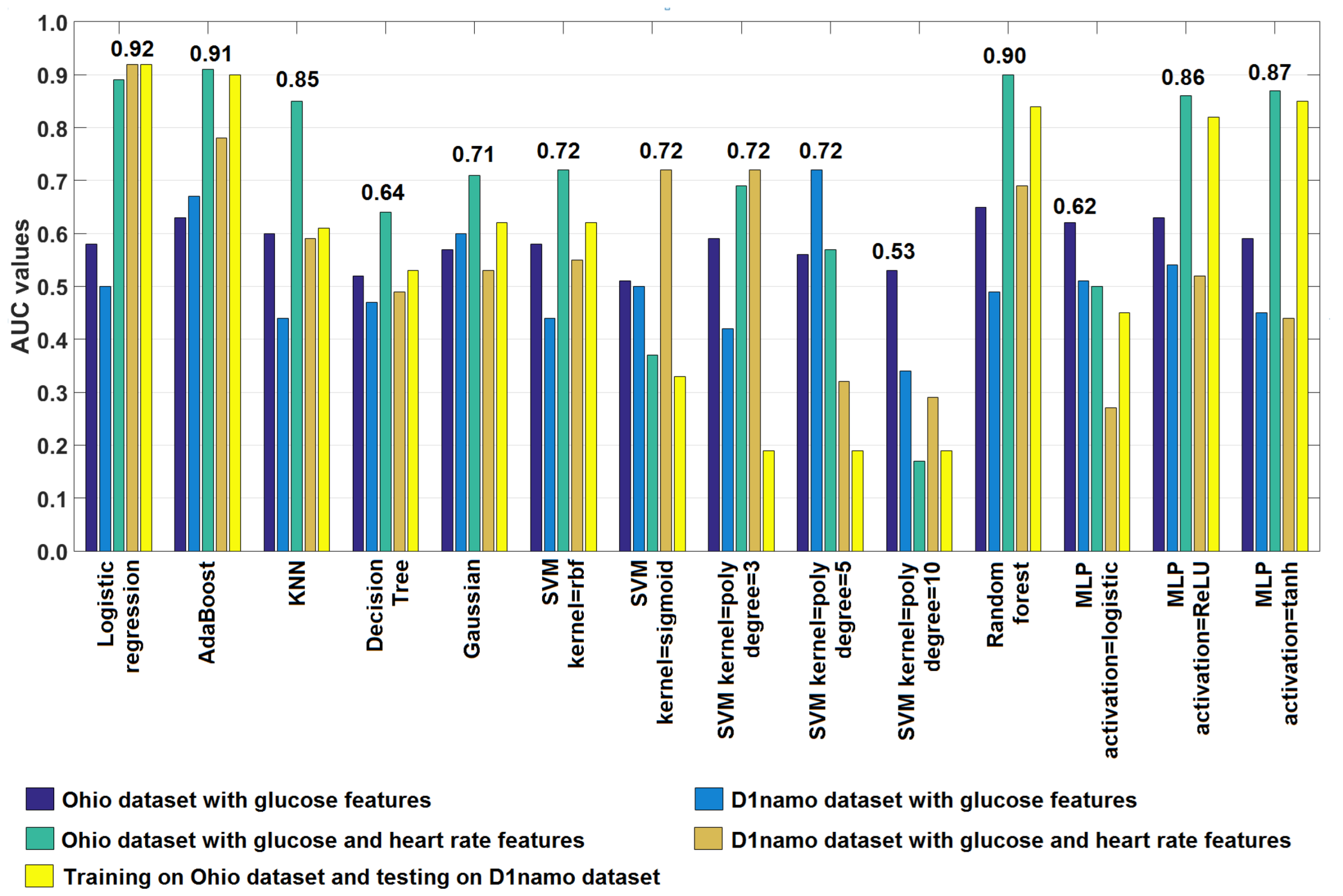
| Training Dataset | Ohio T1DM | D1namo | Ohio T1DM | D1namo | Ohio T1DM |
|---|---|---|---|---|---|
| Testing Dataset | Ohio T1DM | D1namo | Ohio T1DM | D1namo | D1namo |
| Features | BG Only | BG Only | BG and HR | BG and HR | BG and HR |
| Logistic Regression | 0.58 | 0.50 | 0.89 | 0.92 | 0.92 |
| AdaBoost | 0.63 | 0.67 | 0.91 | 0.78 | 0.90 |
| KNN | 0.60 | 0.44 | 0.85 | 0.59 | 0.61 |
| Decision Tree | 0.52 | 0.47 | 0.64 | 0.49 | 0.53 |
| Gaussian | 0.57 | 0.60 | 0.71 | 0.53 | 0.62 |
| SVM kernel = rbf | 0.58 | 0.44 | 0.72 | 0.55 | 0.62 |
| SVM kernel = sigmoid | 0.51 | 0.50 | 0.37 | 0.72 | 0.33 |
| SVM kernel = poly, degree = 3 | 0.59 | 0.42 | 0.69 | 0.72 | 0.19 |
| SVM kernel = poly, degree = 5 | 0.56 | 0.72 | 0.57 | 0.32 | 0.19 |
| SVM kernel = poly, degree = 10 | 0.53 | 0.34 | 0.17 | 0.29 | 0.19 |
| Random Forest | 0.65 | 0.49 | 0.90 | 0.69 | 0.84 |
| MLP activation = logistic | 0.62 | 0.51 | 0.50 | 0.27 | 0.45 |
| MLP activation = ReLU | 0.63 | 0.54 | 0.86 | 0.52 | 0.82 |
| MLP activation = tanh | 0.59 | 0.45 | 0.87 | 0.44 | 0.85 |
Publisher’s Note: MDPI stays neutral with regard to jurisdictional claims in published maps and institutional affiliations. |
© 2022 by the authors. Licensee MDPI, Basel, Switzerland. This article is an open access article distributed under the terms and conditions of the Creative Commons Attribution (CC BY) license (https://creativecommons.org/licenses/by/4.0/).
Share and Cite
Dénes-Fazakas, L.; Siket, M.; Szilágyi, L.; Kovács, L.; Eigner, G. Detection of Physical Activity Using Machine Learning Methods Based on Continuous Blood Glucose Monitoring and Heart Rate Signals. Sensors 2022, 22, 8568. https://doi.org/10.3390/s22218568
Dénes-Fazakas L, Siket M, Szilágyi L, Kovács L, Eigner G. Detection of Physical Activity Using Machine Learning Methods Based on Continuous Blood Glucose Monitoring and Heart Rate Signals. Sensors. 2022; 22(21):8568. https://doi.org/10.3390/s22218568
Chicago/Turabian StyleDénes-Fazakas, Lehel, Máté Siket, László Szilágyi, Levente Kovács, and György Eigner. 2022. "Detection of Physical Activity Using Machine Learning Methods Based on Continuous Blood Glucose Monitoring and Heart Rate Signals" Sensors 22, no. 21: 8568. https://doi.org/10.3390/s22218568