
Evaluation of Calibration Equations by Using Regression Analysis: An Example of Chemical Analysis


Abstract
:1. Introduction
2. Materials and Methods
2.1. Regression Analysis
- Linear equationsy = a0 + a1x
- Higher order polynomial equationsy = bo + b1x + b2x2 + … + bkxk
- Exponential rise to maximum equations (ERTM equations)y = c1 (1 − Exp(c2x))
- Exponential rice to maximum equations with intercepty = do + d1 (1 − Exp(d2x))
- Power equationsy = e1xe2
- Power equations with intercepty = fo + fixf2
2.2. Evaluation Criteria for Calibration Equations
2.2.1. The Criteria of Fitting-Agreement
2.2.2. Criteria for Prediction
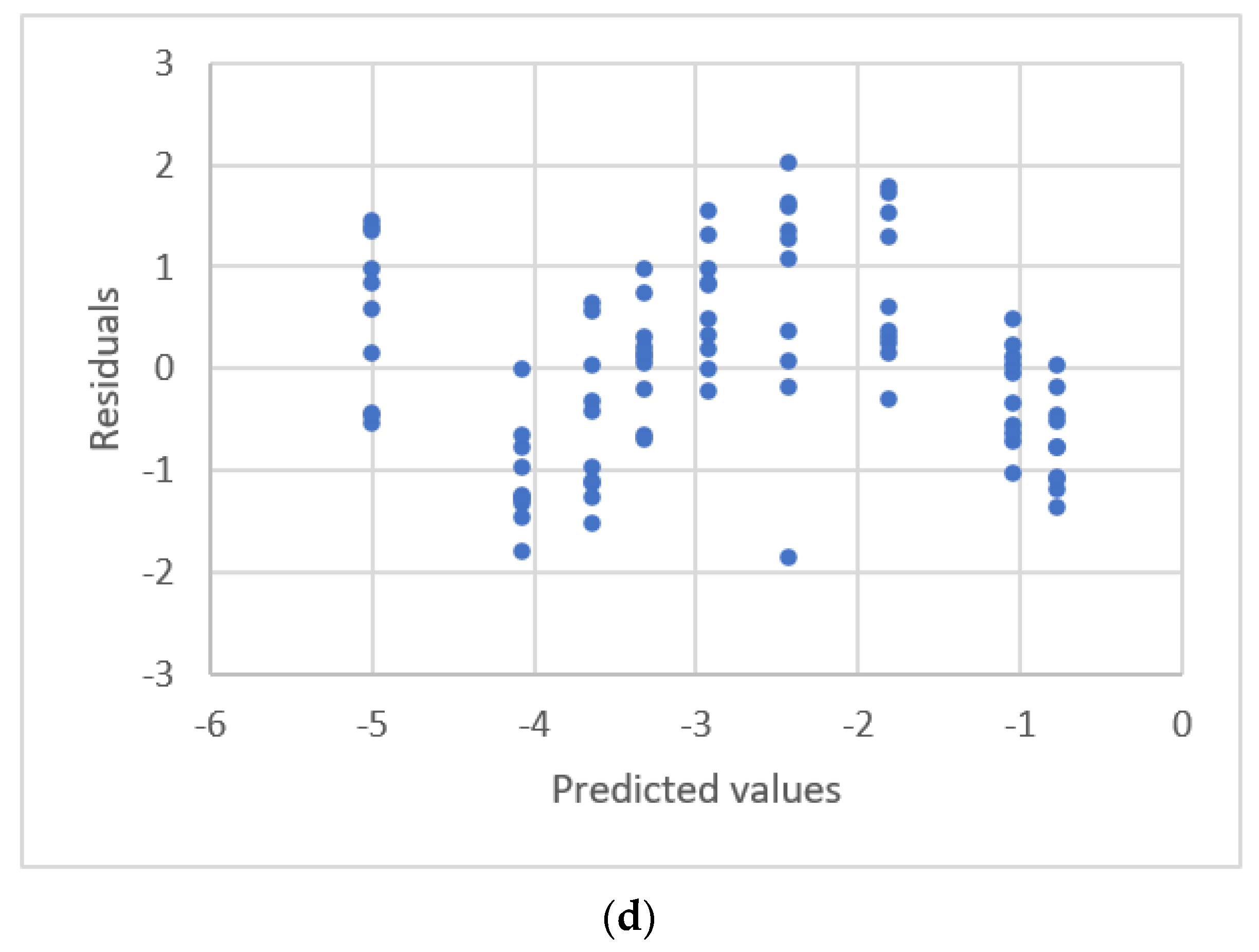
2.3. Residual Plots
2.4. Constant Variance Test
2.5. Transformation
2.6. The Test on a Single Regression Coefficient
2.7. Outlier Test
2.8. Data Sources for Calibration Curves
3. Results
- a.
- Linear equations
- b.
- Nonlinear equations
- c.
- Calibration equations with non-constant variance
- d.
- Calibration curves with outliers
3.1. Linear Equations
3.2. Nonlinear Equations
3.2.1. Quadratic Equations
3.2.2. The 4th Order Polynomial Equations
3.2.3. Exponential Rise to Maximum Equations
3.2.4. Power Equations
3.2.5. Evaluation of Other Data Sets
3.3. Calibration Equations with Non-Constant Variance
3.3.1. The Data Set of Lavagnimi and Magno
y = 6.654 ∗ 10−3 Exp(2.766x0.310)
3.3.2. Other Cases Using the Transformation of the y-Value
s = 0.42, PRESS = 5.28
3.4. Calibration Curves with Outliers
3.5. The Adequate Calibration Equations with the Data Sets Obtained with Same Equipment and Laboratory
3.5.1. Data Sets of Desharnais et al
- Cocainey = 29.979(1 − Exp(−0.0008x))
- Naltrexone
3.5.2. Data Sets of Kirkup and Mulholland
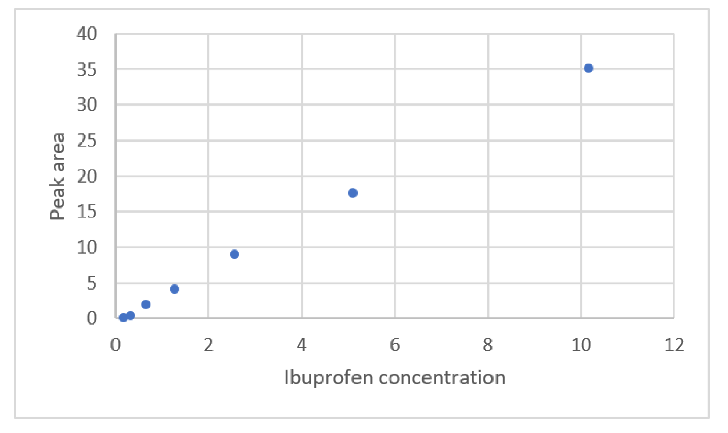
- Ibuprofeny = 0.640 + 3.935x0.953
- Genisteny = −0.640 + 3.935x0.953
- Biovhaniny = −0.475 + 835.467(1 − Exp(−0.0042x))
- Pseudoephedriney = 1930.801 + 430.374x + 0.153x2
- Sodium nitratey = 8263.744x1.033
3.5.3. Data Sets of Martin et al
- Mepy = 207336558.2x0.00000472
- HBCDDy = 105.9236x1.0132
- PFOSy = 32006.765 + 2267.574x − 6.689x2
- PFPeAy = 20650.147 + 8660.301x − 4.0249x2 − 0.0011x3
- PrPy = −18410.374 + 10679965.5 (1 − Exp(−0.0002x))
- PFHpAy = 187092.785 + 26629692.6 (1 − Exp(−0.0008x))
- EtPy = 2768.698 + 1231.0322x − 0.493x2 − 0.0030x3
- PFOAy = 46279.18 x0.773
4. Discussion
5. Conclusions
Author Contributions
Funding
Institutional Review Board Statement
Informed Consent Statement
Acknowledgments
Conflicts of Interest
References
- EURACHEM Working Group. The Fitness for Purpose of Analytical Methods. A Laboratory Guide to Method Validation and Related Topics, 1st ed.; EURACHEM: London, UK, 1998. [Google Scholar]
- IUPAC. Recommendation, guidelines for calibration in analytical chemistry. Part I. Fundamentals and single component calibration. Pure Appl. Chem. 1998, 70, 993–1014. [Google Scholar] [CrossRef]
- Sanagi, M.M.; Nasir, Z.; Ling, S.L.; Hermawan, D.; Ibrahim, W.A.W.; Naim, A.A. A practical approach for linearity assessment of calibration curves under the International Union of Pure and Applied Chemistry (IUPAC) Guidelines for an in-house validation of method of analysis. J. AOAC Intern. 2010, 93, 1322–1330. [Google Scholar] [CrossRef] [Green Version]
- Barwick, V. Preparation of Calibration Curves: A Guide to Best Practice; VAM, LGC/VAM/2003/032. 2003. Available online: http://www.nmschembio.org.uk/dm_documents/LGCVAM2003032_xsJGL.pdf (accessed on 30 October 2021).
- Rozet, E.; Ceccato, A.; Hubert, C.; Ziemons, E.; Oprean, R.; Rudaz, S.; Boulanger, B.; Hubert, P. Analysis of recent pharmaceutical regulatory documents on analytical method validation. J. Chromatogr. A 2007, 1158, 111–125. [Google Scholar] [CrossRef] [PubMed]
- Dux, J.P. Handbook of Quality Assurance for the Analytical Chemistry Laboratory, 2nd ed.; Van Nostrand Reinhold: New York, NY, USA, 1990. [Google Scholar]
- Miller, J.N. Basic statistical methods for analytical chemistry Part 2. Calibration and regression methods—A Review. Analyst 1991, 116, 3–14. [Google Scholar] [CrossRef]
- Boqué, R.; Rius, F.X.; Massart, D.L. Straight line calibration: Something more than slopes, intercepts, and correlation coefficients. J. Chem. Educ. 1993, 70, 230–232. [Google Scholar] [CrossRef]
- Santovito, E.; Elisseeva, S.; Cruz-Romero, M.C.; Duffy, G.; Kerry, J.P.; Papkovsky, D.B. A Simple sensor system for onsite monitoring of O2 in vacuum-packed meats during the shelf life. Sensors 2021, 21, 4256. [Google Scholar] [CrossRef]
- Bruggemann, L.; Wennrich, R. Design and model of calibration for chemical measurements. Accred. Qual. Assur. 2008, 13, 567–573. [Google Scholar] [CrossRef]
- Rozet, E.; Ziemons, E.; Marini, R.D.; Hubert, P. Usefulness of information criteria for the selection of calibration curves. Anal. Chem. 2013, 85, 6327–6335. [Google Scholar] [CrossRef] [PubMed]
- Raposo, F. Evaluation of analytical calibration based on least-squares linear regression for instrumental techniques: A tutorial review. Trends Anal. Chem. 2016, 77, 167–185. [Google Scholar] [CrossRef]
- Moosavi, S.M.; Ghassabian, S. Linearity of calibration curves for analytical methods: A review of criteria for assessment of method reliability. In Calibration and Validation of Analytical Methods—A Sampling of Current Approaches; IntechOpen Ltd.: London, UK, 2018; pp. 109–127. [Google Scholar]
- Cuadros Rodrıguez, L.; Garcıa Campana, A.M.; Jimenez Linares, C.; Roman Ceba, M. Estimation of performance characteristics of an analytical method using the data set of the calibration experiment. Anal. Lett. 1993, 26, 1243–1258. [Google Scholar] [CrossRef]
- Huber, M.K.W. Improved calibration for wide measuring ranges and low contents. Accred. Qual. Assur. 1997, 2, 367–374. [Google Scholar] [CrossRef]
- Mulholland, M.; Hibbert, D.B. Linearity and the limitations of least squares calibration. J. Chromatogr. A 1997, 762, 73–82. [Google Scholar] [CrossRef]
- Desimoni, E. A program for the weighted linear least-squares regression of unbalanced response arrays. Analyst 1999, 124, 1191–1196. [Google Scholar] [CrossRef]
- Kirkup, L.; Mulholland, M. Comparison of linear and non-linear equations for univariate calibration. J. Chromatogr. A 2004, 1029, 1–11. [Google Scholar] [CrossRef]
- Bruggemann, L.; Quapp, W.; Wennrich, R. Test for non-linearity concerning linear calibrated chemical measurements. Accred. Qual. Assur. 2006, 11, 625–631. [Google Scholar] [CrossRef]
- Lavagnini, I.; Magno, F. A statistical overview on univariate calibration, inverse regression, and detection limits: Application to gas chromatography/mass spectrometry technique. Mass Spectrom. Rev. 2007, 26, 1–18. [Google Scholar] [CrossRef] [PubMed]
- Ortiz, M.C.; Sánchez, M.S.; Sarabia, L.A. Quality of analytical measurements: Univariate regression. In Comprehensive Chemometrics. Chemical and Biochemical Data Analysis; Brown, S.D., Tauler, R., Walczak, B., Eds.; Elsevier: Amsterdam, The Netherlands, 2009; pp. 127–169. [Google Scholar]
- Rawski, R.I.; Sanecki, P.T.; Kijowska, K.M.; Skital, P.M.; Saletnik, D.E. Regression analysis in analytical chemistry. Determination and validation of linear and quadratic regression dependencies. S. Afr. J. Chem. 2016, 69, 166–173. [Google Scholar] [CrossRef]
- Desharnais, B.; Camirand-lemyre, F.; Mireault, P.; Skinner, C.D. Procedure for the selection and validation of a calibration model I—Description and application. J. Anal. Toxicol. 2017, 41, 261–268. [Google Scholar] [CrossRef] [PubMed]
- Martin, J.; de Adana, D.D.R.; Asuero, A.G. Fitting models to data: Residual analysis, a primer. In Uncertainty Quantification and Model Calibration; Hessling, J.P., Ed.; IntechOpen Ltd.: London, UK, 2017; Chapter 7; p. 133. [Google Scholar]
- Hinshaw, J.V. Non-linear calibration. LC GC Eur. 2002, 15, 2–5. [Google Scholar]
- Lavín, Á.; Vicente, J.D.; Holgado, M.; Laguna, M.F.; Casquel, R.; Santamaría, B.; Maigler, M.V.; Hernández, A.L.; Ramírez, Y. On the determination of uncertainty and limit of detection in label-free biosensors. Sensors 2018, 18, 2038. [Google Scholar] [CrossRef] [Green Version]
- Machado, J.; Carvalho, P.M.; Félix, A.; Doutel, D.; Santos, J.P.; Carvalho, M.L.; Pessanha, S. Accuracy improvement in XRF analysis for the quantification of elements ranging from tenths to thousands mg g−1 in human tissues using different matrix reference materials. J. Anal. At. Spectrom. 2020, 35, 2920. [Google Scholar] [CrossRef]
- Pagliano, E.; Meija, J. A tool to evaluate nonlinearity in calibration curves involving isotopic internal standards in mass spectrometry. Int. J. Mass Spectrom. 2021, 464, 116557. [Google Scholar] [CrossRef]
- Mrozek, P.; Gorodkiewicz, E.; Falkowski, P.; Hościło, B. Sensitivity analysis of single- and bimetallic surface plasmon resonance biosensors. Sensors 2021, 21, 4348. [Google Scholar] [CrossRef]
- Frisbie, S.H.; Mitchell, E.J.; Sikora, K.R.; Abualrub, M.S.; Abosalem, Y. Using polynomial regression to objectively test the fit of calibration curves in analytical chemistry. Int. J. Appl. Mat. Theor. Phys. 2005, 1, 14–18. [Google Scholar] [CrossRef]
- Martin, J.; Gracia, A.R.; Asuero, A.G. Fitting nonlinear calibration curves: No models perfect. J. Anal. Sci. Methods Instrum. 2017, 7, 1–17. [Google Scholar] [CrossRef] [Green Version]
- Kohl, M.; Stepath, M.; Bracht, T.; Megger, D.A.; Sitek, B.; Marcus, K.; Eisenacher, M. CalibraCurve: A tool for calibration of targeted MS-based measurements. Proteomics 2020, 22, e1900143. [Google Scholar] [CrossRef] [PubMed]
- Myers, R.H. Classical and Modern Regression with Applications, 2nd ed.; Duxbury Press: Monterey, CA, USA, 1990. [Google Scholar]
- Weisberg, S. Applied Linear Regression, 4th ed.; Wiley: New York, NY, USA, 2013; p. 384. [Google Scholar]
- Alexander, D.L.J.; Tropsha, A.; Winkler, D.A. Beware of R2: Simple, unambiguous assessment of the prediction accuracy of QSAR and QSPR models. J. Chem. Inf. Model. 2015, 55, 1316–1322. [Google Scholar] [CrossRef] [Green Version]
- Kvalseth, T.O. Cautionary note about R2. Am. Stat. 1985, 39, 279–285. [Google Scholar]
- Anderson-Sprecher, R. Model comparisons and R2. Am. Stat. 1994, 48, 113–117. [Google Scholar]
- Montgomery, D.C.; Peck, E.A.; Vining, C.G. Introduction to Linear Regression Analysis, 5th ed.; John Wiley & Sons, Inc.: New York, NY, USA, 2012; p. 836. [Google Scholar]
- Rawlings, J.O.; Pantula, S.G.; Dickey, D. Applied regression analysis. In Springer Texts in Statistics; Springer: New York, NY, USA, 1998. [Google Scholar]
- Kutner, M.H.; Nachtsheim, J.; Neter, J. Applied Linear Regression Models, 4th ed.; McGraw-Hill: New York, NY, USA, 2004; Volume 17. [Google Scholar]
- Njaka, N.A.; Elise, O.R.; Herinirina, N.R.; Lucienne, V.R.; Manovantsoatsiferana, H.R.A.; Randrianarivony, E. Dealing with outlier in linear calibration curves: A case study of graphite furnace atomic absorption spectrometry. World J. Appl. Chem. 2018, 3, 10–16. [Google Scholar]
- Pop, I.S.; Pop, V.; Cobzac, S.; Sârbu, S. Use of weighted least-squares splines for calibration in analytical chemistry. J. Chem. Inf. Comput. Sci. 2000, 40, 91–98. [Google Scholar] [CrossRef]
- Asuero, A.G.; González, G. Fitting straight lines with replicated observations by linear regression. III. Weighting Data. Crit. Rev. Anal. Chem. 2007, 37, 143–172. [Google Scholar] [CrossRef]
- Deaton, M.L.; Reynolds, M.R.; Myers, R.H. Estimation and hypothesis testing in regression in the presence of nonhomogeneous error variances. Commun. Stat. B 1983, 12, 45–66. [Google Scholar] [CrossRef]
- Dos Santos, M.I.R.; Porta Nova, A.M. Statistical fitting and validation of non-linear simulation metamodels: A case study. Eur. J. Oper. Res. 2006, 171, 53–63. [Google Scholar] [CrossRef]
- Yang, X.J.; Low, G.K.C.; Foley, R. A novel approach for the determination of detection limits for metal analysis of environmental water samples. Anal. Bioanal. Chem. 2005, 381, 1253–1263. [Google Scholar] [CrossRef]
- Lu, H.; Chen, C. Uncertainty evaluation of humidity sensors calibrated by saturated salt solutions. Measurement 2007, 40, 591–599. [Google Scholar] [CrossRef]
- Chen, C. Evaluation of measurement uncertainty for thermometers with calibration equations. Accred. Qual. Assur. 2006, 11, 75–82. [Google Scholar] [CrossRef] [Green Version]
- Hsu, K.; Chen, C. The effect of calibration equations on the uncertainty of UV-Vis spectrophotometric measurement. Measurement 2010, 43, 1525–1531. [Google Scholar] [CrossRef]
- Chen, H.; Chen, C. On the use of modern regression analysis in liver volume prediction equation. J. Med. Imaging Health Inform. 2017, 7, 338–349. [Google Scholar] [CrossRef]
- Wang, C.; Chen, C. Use of modern regression analysis in plant tissue culture. Propag. Ornam. Plants 2017, 17, 83–94. [Google Scholar]
- Chen, C. Relationship between water activity and moisture content in floral honey. Foods 2019, 8, 30. [Google Scholar] [CrossRef] [PubMed] [Green Version]
- Weng, Y.K.; Chen, J.; Cheng, C.W.; Chen, C. Use of modern regression analysis in the dielectric properties of foods. Foods 2020, 9, 1472. [Google Scholar] [CrossRef] [PubMed]


| Study | Equipment | Target | Standard, Range | Response Range | Calibration Equation | Statistic Criteria |
|---|---|---|---|---|---|---|
| Mulholland and Hibbert [16] | HPLC 1 | Diadzen | 0.162–10.96 mg/50 mL | 0.243–30.75 Peak area | Linear y = X1.1 | R2, Residual plot |
| Desimoni [17] | Flow injection analysis | sulfides | 0.88–81.2 μm | 0.170–15.94 μA | linear | R2, Residual plot |
| Yang et al. [46] | ICP-MP 2 | CD(114) | 0–25,000 ng/L | −53.9–25,726 | polynomial | Outliers, s |
| Bruggemann et al. [19] | ICP Spectrometer | Aresenic | 0~10.0 ng/L | −92~26,394 | Linear polynom | R2, s, Lack of fit, Residual plot |
| Lavagnini & Magno [20] | GC MS 3 | Chloromethanre | 0~4 μg/L | 0.111975~ 0.465813 Peak area ratio | Linear polynomial | s, Residual plot |
| Ortiz et al. [21] | Ex1. HPLC-DAP 4 Ex2. Anodic Stripping voltammetry | Ascorbic Cadmium | 0.004–0.026 mg/L 20.18~60.08 nmol/L | 14.54–83.5 Peak area 4.50~15.98 nA | linear linear | s ANOVA, R2,Residual plots |
| Ex3. SWADS using DMG 5 | Nickel | 0~415 μmol/L | 2.5~76.87 μA | linear | R2 | |
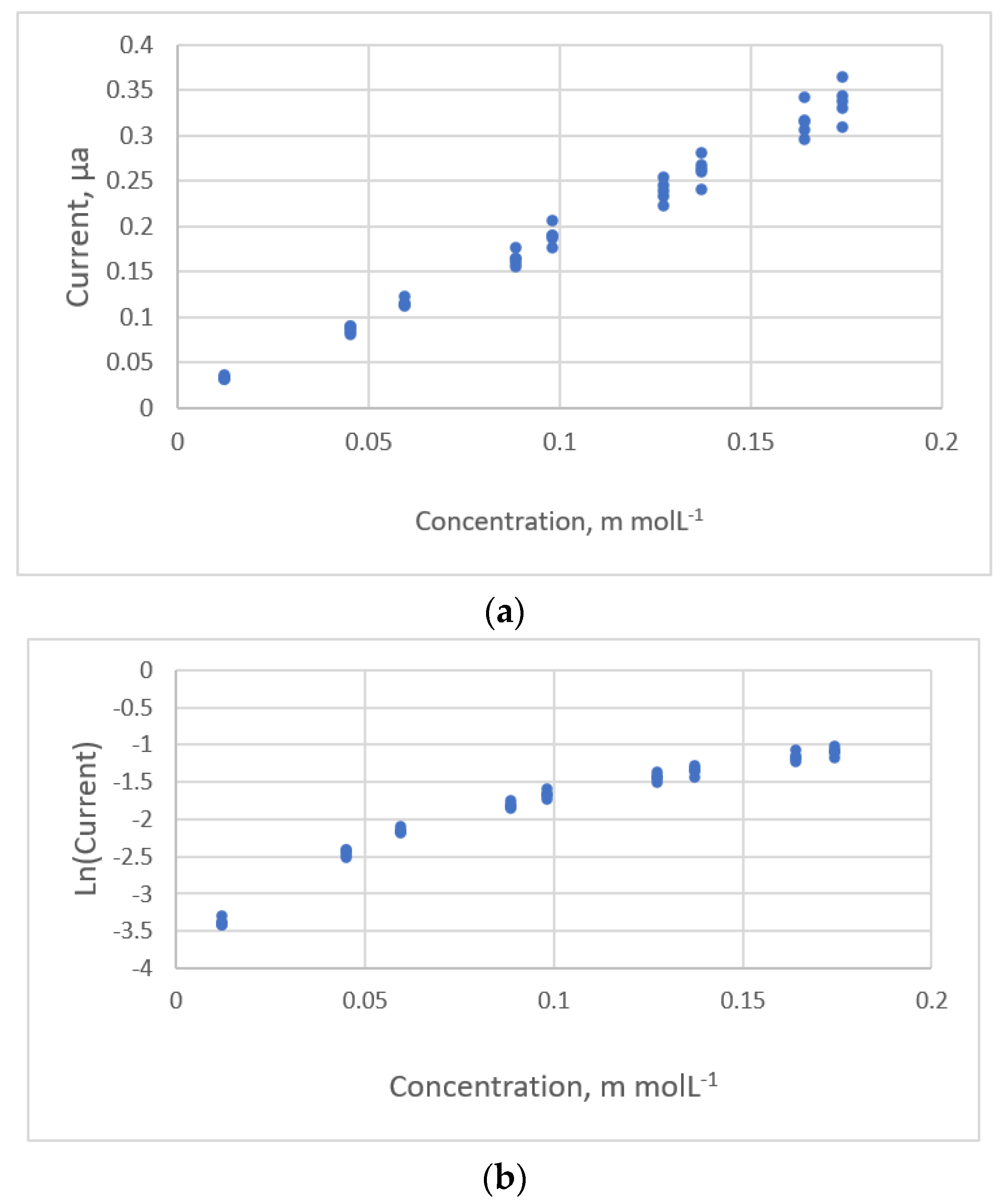
| Ex4. Pulse Polarography | Benzaldehyde | 0.0198~0.1740 mnol/L | 0.033~0.366 μA | linear | Residual plots, s | |
| Kirkup and Mulholl-and [18] | HPLC | Ibuprofen Genisten Biochanin Pseudoephedrine Sodium nitrate | 103.9~305.7 ng 0.159~10.16 mg 0.158~10.09 mg 61.4~181.5 mg 1.006~25.16 | Area 261.357~755.89 0.15508~35.2175 0.12111~34.0687 28,653~85,241 8103~233,405 | Linear polynomicl Y = a + bxm | R2, Radj2, ANOVA, AIC 9, residual plots |
| Rawski et al. [22] | Spectrophotomethic | Albumin | 0~20 μg/mL | 0~450 Peak height × 10−3 | Linear | Lack of fit, R2 |
| Desharnais et al. [17] | LC-MS 6 | Cocaine Naltrexone | 5~1000 ng/mL 5~1000 ng/mL | 0.049~9.209 Area ratio 0.226~16.298 Area ratio | Linear linear | Partial F-test, ANOVA Partial F-test, ANOVA |
| Martin et al. [24] | Ex1. HPLC | Vitamin B12 | 0.23~4.0 ng | 0.14~1.29 Area ratio | High order polynomial | R2 Residual Plots |
| Ex2. HPLC | Blood | 0~90 ng/mL | 0.002~0.272 Area ratio | |||
| Martin et al. [31] | LC-QqQ-MS 7 | MeP | 1–1500 ng/mL | 864–1,470,121 | linear | R2 |
| arsay | HBCDD | 1–1500 ng/mL | 105–175,247 | |||
| PFOS | 2548–1,924,470 | |||||
| PFPeA | 9110–7,597,353 | |||||
| PrP | 2150–3,054,469 | |||||
| PFHpA | 29,847–19,417,533 | |||||
| EtP | 1007–2,062,210 | |||||
| PFOA | 12,569–12,906,640 | |||||
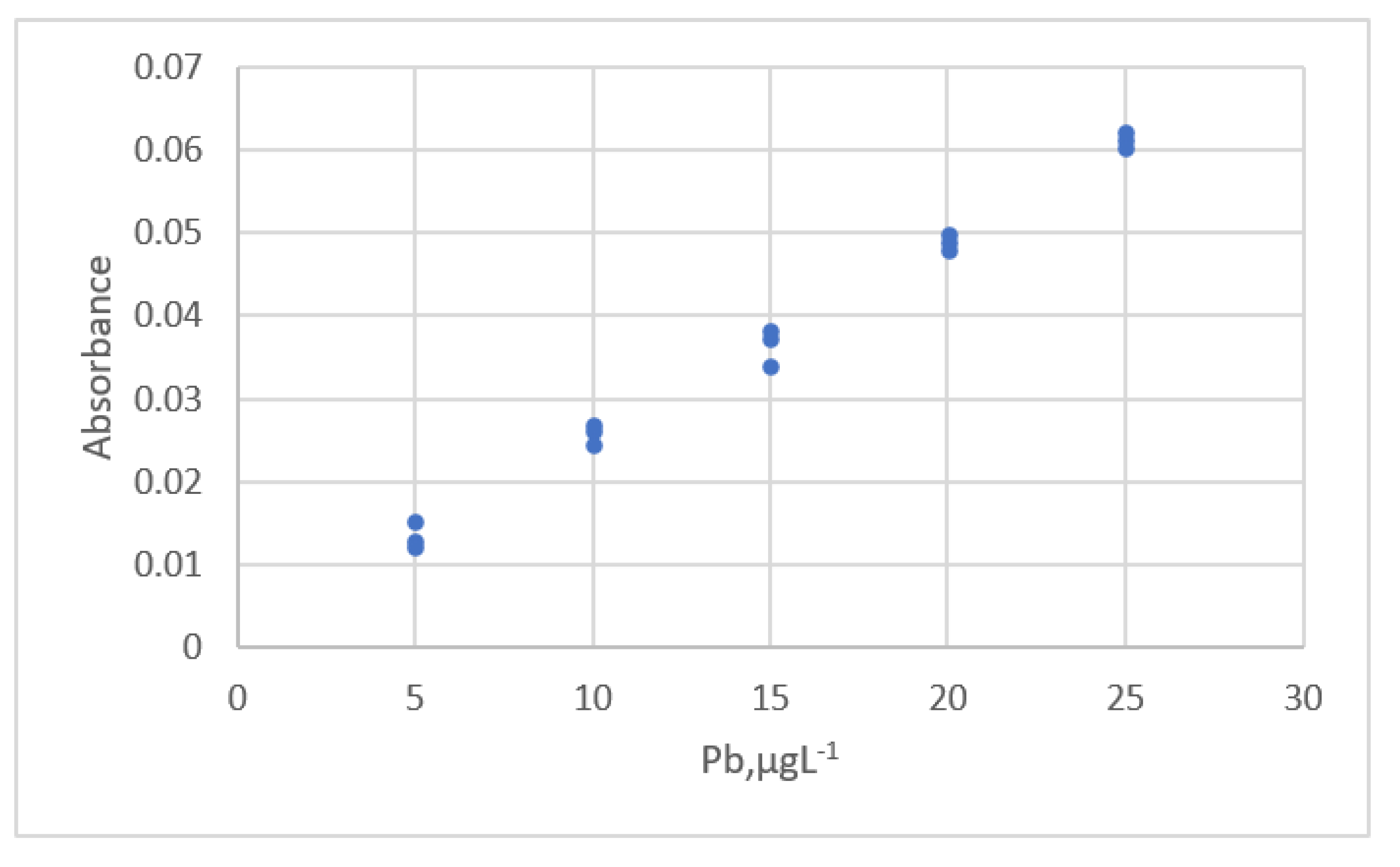
| Njaka et al. [41] | GF-AAS 8 | Pb | 5~25 μg/L | 0.0122~0.0622 Absorbanc | linear | R2 Outliers., Residual plots. |
| Lavin et al. [26] | Ex1.Jmmunoassay moden | unknow | 0~500 μg/mL | 0~99.2 | polynomial | AICs 10, R2 |
| Ex2. Biophotonic sensing cells | Anti-IgG | 1~100 μg/mL | 0.00~6.14 | polynomial | AICs, R2 |
| Equation | s | PRESS | Residual Plots |
|---|---|---|---|
| 1. y = 222.512 + 30812x | 89.644 | 160,637 | Uniform distribution |
| 2. y = 191.243 + 313946.6x − 199117.011x2 | 92.034 | 182,248 | U.D. |
| 3. y = 48234.378(1 − Exp(−7.150x)) | 102.857 | 220,533 | U.D. |
| 4. y = 188.052 + 222889.55(1 − Exp(−1.4113x)) | 92.037 | 182,214 | U.D. |
| 5. y = 255791.66x0.9426 | 92.241 | 176,843 | U.D. |
| 6. y = 160.955 + 290978.8x0.983 | 92.017 | 179,136 | U.D. |
| Equation | s | PRESS | Residual Plots |
|---|---|---|---|
| 1. y = −0.172 + 2.818x | 0.315 | 4.140 | Fixed pattern |
| 2. y = −0.414 + 3.0801x−0.0241x2 | 0.225 | 2.418 | U.D. |
| 3. y = 624.382(1 − Exp(−0.0046x)) | 0.335 | 4.498 | Fixed pattern |
| 4. y = −0.417 + 182.166(1 − Exp(−0.0169x)) | 0.225 | 2.259 | U.D. |
| 5. y = 2.806x0.998 | 0.334 | 4.814 | Fixed pattern |
| 6. y = −0.543 + 3.237x0.945 | 0.241 | 2.472 | U.D. |
| Equation | s | PRESS | Residual Plots |
|---|---|---|---|
| 1. y = 9.832 + 192.469x | 7.587 | 1299.3 | Fixed pattern |
| 2. y = −2.861 + 383.458x − 459.414x2 | 2.986 | 231.49 | Fixed pattern |
| 3. y = 1.620 + 235.042x + 452.872x2 − 1455.64x3 | 1.707 | 81.364 | Fixed pattern |
| 4. y = 3.347 + 124.632x + 1733.643x2 − 6367.25x3 + 5939.812x4 | 1.360 | 70.125 | U.D. |
| 5. y = 103.107(1 − Exp(−3.712x)) | 3.982 | 361.11 | Fixed pattern |
| 6. y = −2.975 + 101.749(1 − Exp(−4.150x)) | 3.966 | 434.6 | Fixed pattern |
| 7. y = 155.549x0.686 | 5.692 | 740.4 | Fixed pattern |
| 8. y = −3.401 + 155.388x0.644 | 5.716 | 1919.1 | Fixed pattern |
| Equation | s | PRESS | Residual Plots |
|---|---|---|---|
| 1. y = 47.773 + 22.047x | 27.408 | 7431 | Fixed pattern |
| 2. y = 4.946 + 36.322x − 0.714x2 | 8.766 | 2718 | U.D |
| 3. y = 617.147(1 − Exp(−0.0654x)) | 8.560 | 2611 | U.D |
| 4. y = 0.707 + 618.310(1 − Exp(−0.650x)) | 8.698 | 2672 | U.D |
| 5. y = 57.694x0.696 | 12.781 | 5976 | Fixed pattern |
| 6. y = −7.232 + 61.790x0.678 | 12.766 | 5948 | Fixed pattern |
| Equation | s | PRESS | Residual Plots |
|---|---|---|---|
| 1. y = −0.670 + 3.510x | 0.280 | 1.253 | Fixed pattern |
| 2. y = −0.473 + 3.731x − 0.022x2 | 0.187 | 0.599 | Fixed pattern |
| 3. y = −6319 + 4.074x − 0.125x2 + 0.007x3 | 0.148 | 0.348 | Fixed pattern |
| 4. y = 2128.294(1 − Exp(−0.0016x)) | 0.356 | 1.595 | Fixed pattern |
| 5.y = −0.477 + 296.738(1 − Exp(−0.0126x)) | 0.186 | 0.567 | U.D. |
| 6. y = 3.443x1.004 | 0.354 | 1.737 | U.D. |
| 7. y = −0.640 + 3.935x0.953 | 0.165 | 0.349 | U.D. |
| Equation | s | PRESS | Residual Plots |
|---|---|---|---|
| 1. y = 0.0186 + 0.0972x | 0.0243 | 0.0554 | Fixed pattern |
| 2. y = 0.010133 + 0.128x − 0.00804x2 | 0.0320 | 0.0475 | Fixed pattern |
| 3. y = 0.664 (1 − Exp(−0.222x)) | 0.0227 | 0.0501 | Fixed pattern |
| 4. y = 0.132x0.790 | 0.0221 | 0.0470 | Fixed pattern |
| Equation | s | RESS | Residual Plots |
|---|---|---|---|
| 1. Lny = −4.165 + 2.356x − 0.403x2 | 0.423 | 16.501 | Fixed pattern |
| 2. Lny = −4.373 + 3.837x − 1.544x2 + 0.201x3 | 0.320 | 9.494 | Fixed pattern |
| 3. Lny = −4.561 + 5.986x − 54.802x2 + 1.439x3 − 0.154x4 | 0.242 | 6.811 | U.D. |
| 4. Lny = −4.537 + 3.393x + 1.678x2 | 0.271 | 6.839 | U.D. |
| 5. Lny = −5.0126 + 2.763x0.309 | 0.224 | 4.578 | U.D. |
| Equation | s | PRESS | Residual Plots |
|---|---|---|---|
| 1. y = 0.00364 + 0.00143x | 0.0266 | 0.0415 | U.D. with outlier |
| 2. y = −0.504(1 − Exp(−0.00340x)) | 0.0267 | 0.0420 | U.D. with outlier |
| 3. y = 0.0024x0.893 | 0.0167 | 0.0411 | U.D. with outlier |
| Equation | s | PRESS | Residual Plots |
|---|---|---|---|
| 1. y = 0.00543 + 0.00126x | 0.0165 | 0.0139 | U.D. |
| 2. y = 0.192(1 − Exp(−0.0101x)) | 0.0158 | 0.0142 | U.D. |
| 3. y = 0.00351x0.779 | 0.0161 | 0.0137 | U.D. |
Publisher’s Note: MDPI stays neutral with regard to jurisdictional claims in published maps and institutional affiliations. |
© 2022 by the authors. Licensee MDPI, Basel, Switzerland. This article is an open access article distributed under the terms and conditions of the Creative Commons Attribution (CC BY) license (https://creativecommons.org/licenses/by/4.0/).
Share and Cite
Chen, H.-Y.; Chen, C. Evaluation of Calibration Equations by Using Regression Analysis: An Example of Chemical Analysis. Sensors 2022, 22, 447. https://doi.org/10.3390/s22020447
Chen H-Y, Chen C. Evaluation of Calibration Equations by Using Regression Analysis: An Example of Chemical Analysis. Sensors. 2022; 22(2):447. https://doi.org/10.3390/s22020447
Chicago/Turabian StyleChen, Hsuan-Yu, and Chiachung Chen. 2022. "Evaluation of Calibration Equations by Using Regression Analysis: An Example of Chemical Analysis" Sensors 22, no. 2: 447. https://doi.org/10.3390/s22020447