
Remote Sensing Image Fusion Based on Morphological Convolutional Neural Networks with Information Entropy for Optimal Scale

Abstract
:1. Introduction
2. Multi-Scale MCA Algorithm
2.1. Image Decomposition via MCA
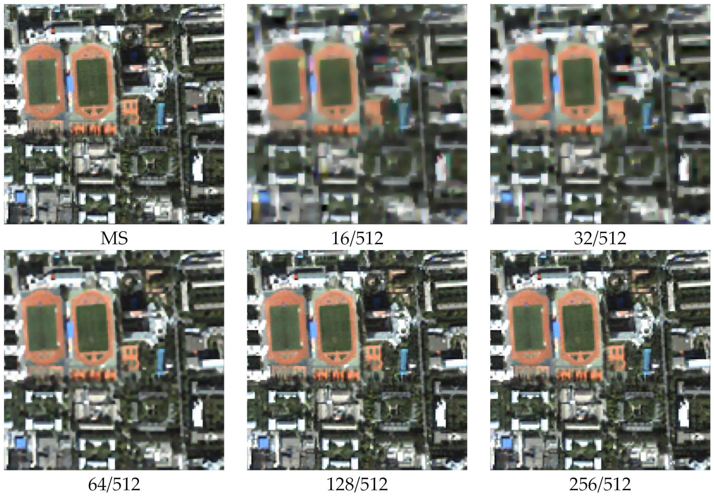
2.2. Decomposition with Different Scales
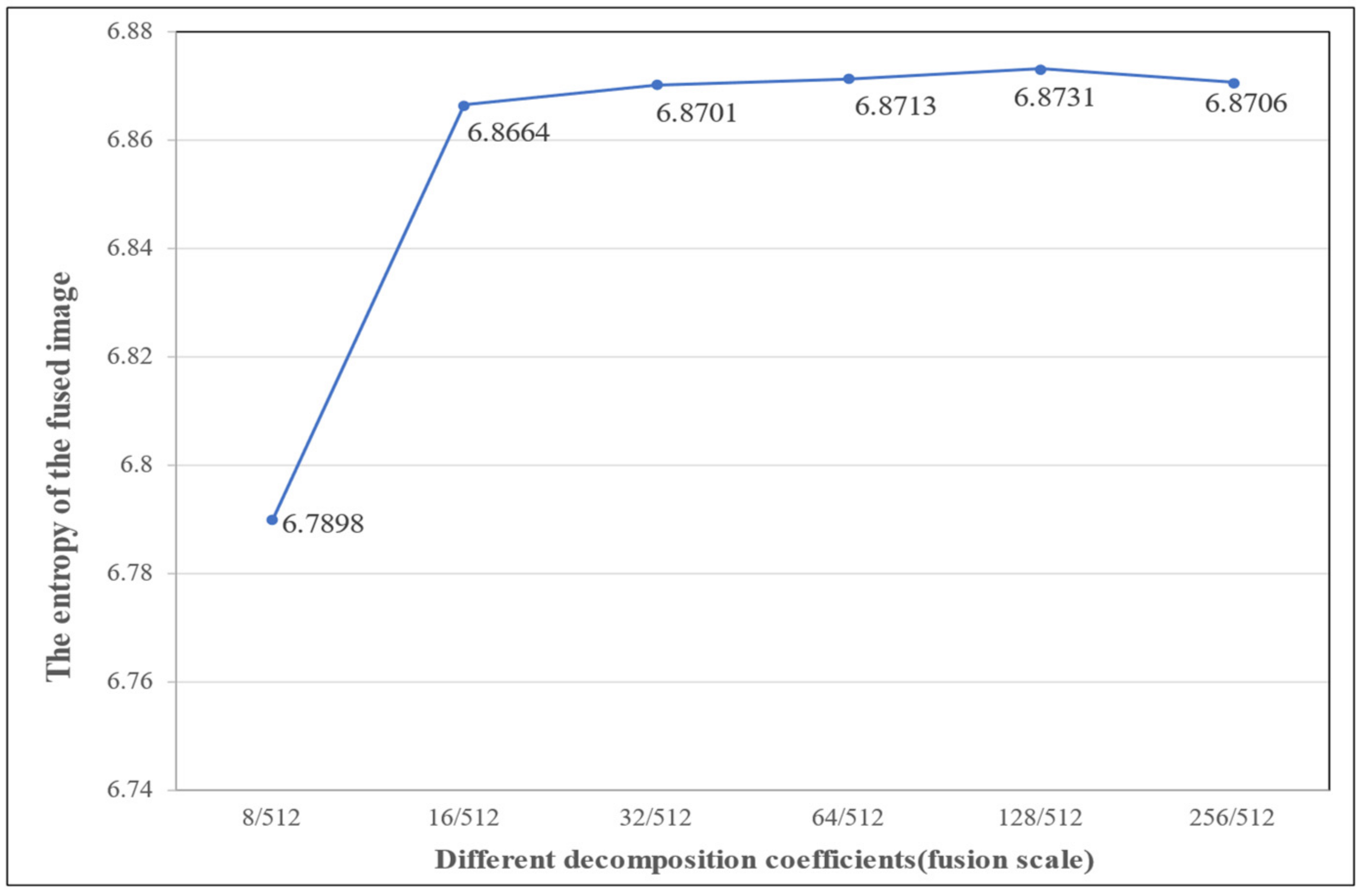
2.3. Information Entropy Metric
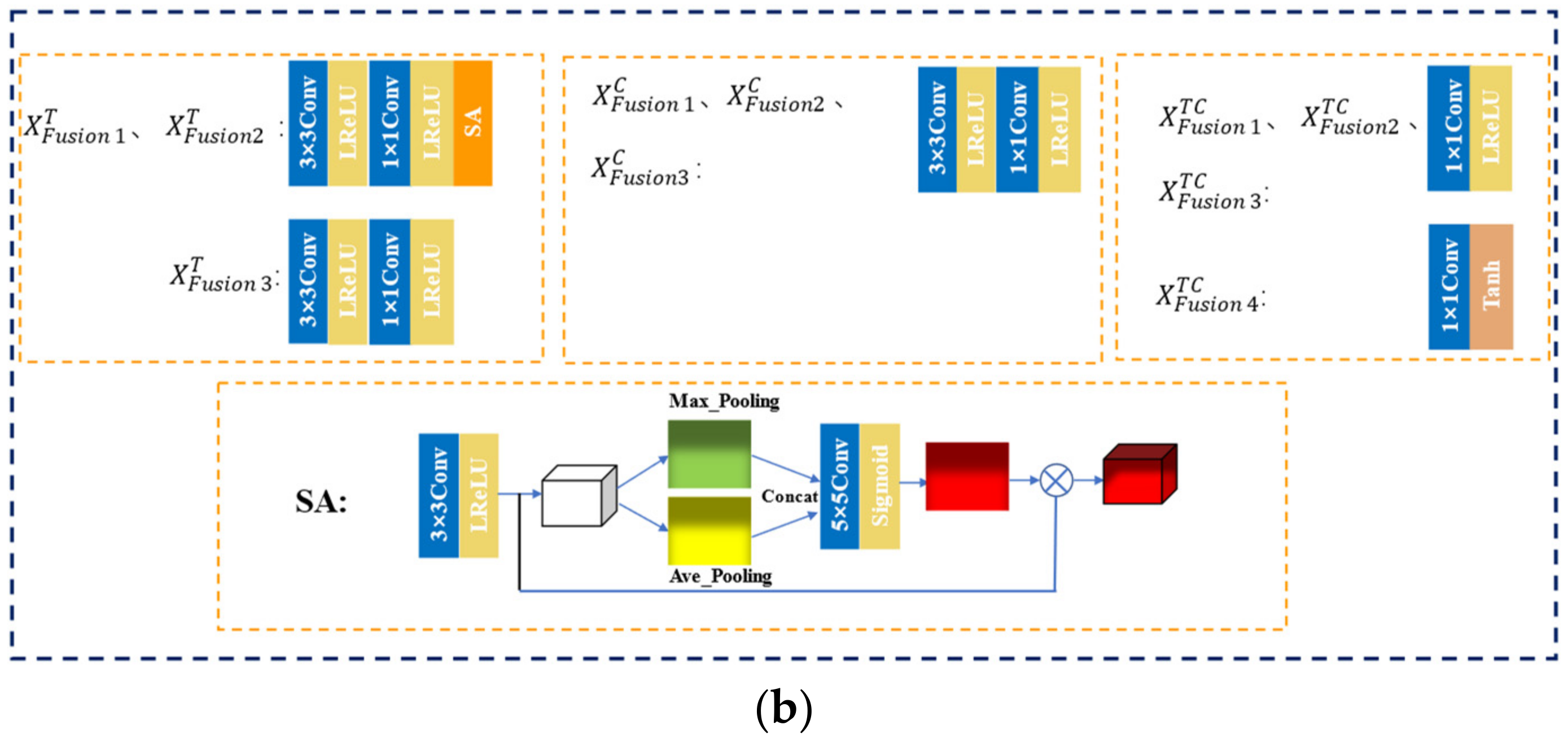
2.4. Multi-Scale Spatial Attention Module
3. Methods
3.1. Network Setup and Multi-Scale Fusion
3.1.1. Algorithm Flow
- A The joint LDCT dictionary and CT dictionary form the decomposition dictionary , and MCA is performed on the input source images PAN and MS at multi-scale to extract the texture component and cartoon components, respectively.
- The threshold values of the parameters are calculated using the information entropy of the fused image from Step 3 to select the best extraction scale for the cartoon component of the MS image and the texture component of the PAN image.
- The optimal-scale cartoon component and texture component are fused by the attentional CNN to produce the final fused image.
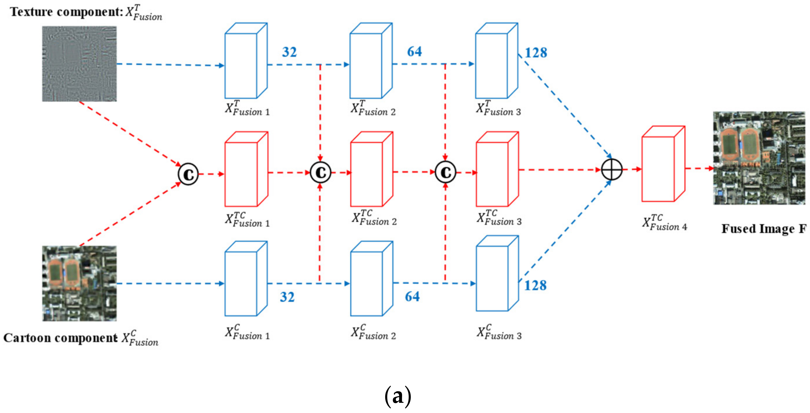
3.1.2. Network Structure
3.1.3. Different Scale Fusion Results
4. Results and Discussion
4.1. Model Training
4.2. Experimental Data
4.3. Evaluation Indexes
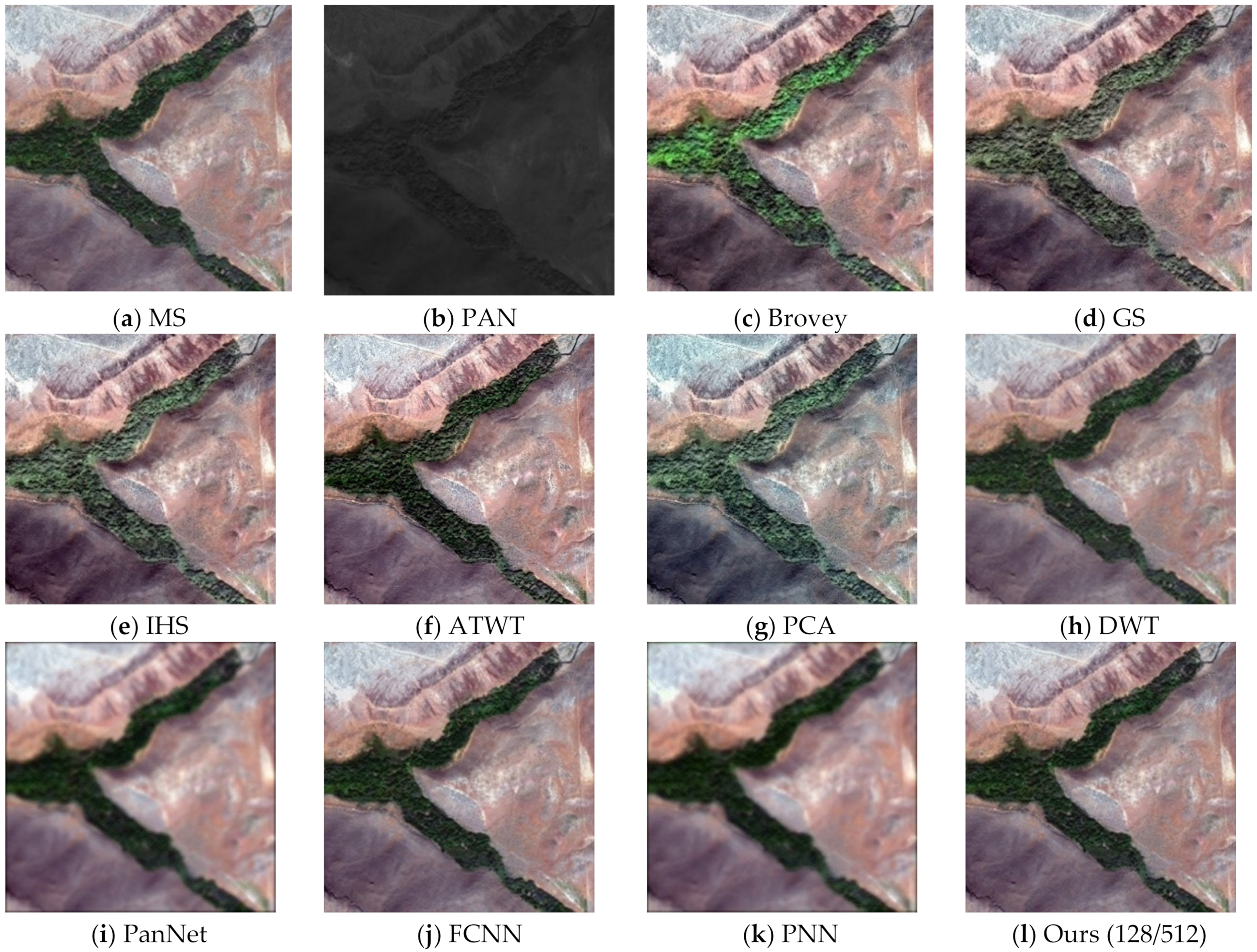
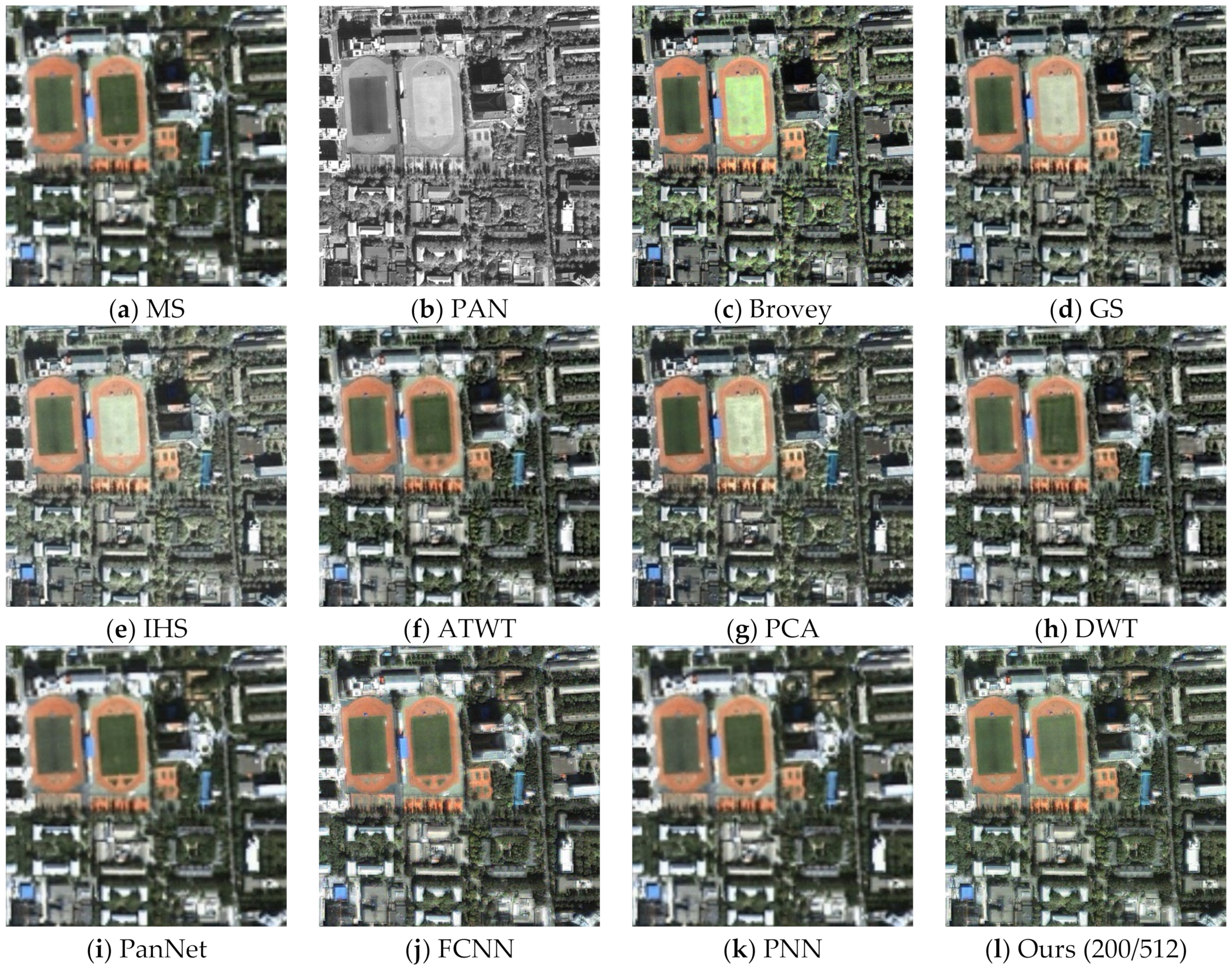
4.4. Experimental Results


5. Conclusions
Author Contributions
Funding
Institutional Review Board Statement
Informed Consent Statement
Data Availability Statement
Conflicts of Interest
References
- Zhou, H.Y.; Liu, Q.J.; Wang, Y.H. PGMAN: An unsupervised generative multiadversarial network for pansharpening. IEEE J. Sel. Top. Appl. Earth Observ. Remote Sens. 2021, 14, 6316–6327. [Google Scholar]
- Choi, J.; Yu, K.; Kim, Y. A new adaptive component-substitution-based satellite image fusion by using partial replacement. IEEE Trans. Geosci. Remote Sens. 2011, 49, 295–309. [Google Scholar]
- Shah, V.P.; Younan, N.H.; King, R.L. An efficient pan-sharpening method via a combined adaptive PCA approach and contourlets. IEEE Trans. Geosci. Remote Sens. 2008, 46, 1323–1335. [Google Scholar]
- Vivone, G.; Simoes, M.; Dalla Mura, M.; Restaino, R.; Bioucas-Dias, J.M.; Licciardi, G.A.; Chanussot, J. Pansharpening based on semiblind deconvolution. IEEE Trans. Geosci. Remote Sens. 2015, 53, 1997–2010. [Google Scholar]
- Li, J.; Sun, W.X.; Jiang, M.H.; Yuan, Q.Q. Self-supervised pansharpening based on a cycle-consistent generative adversarial network. IEEE Trans. Image Process. 2022, 19, 1–5. [Google Scholar]
- Ozcelik, F.; Alganci, U.; Sertel, E.; Unal, G. Rethinking CNN-based pansharpening: Guided colorization of panchromatic images via GANs. IEEE Trans. Geosci. Remote Sens. 2021, 59, 3486–3501. [Google Scholar]
- Deng, L.J.; Vivone, G.; Jin, C.; Chanussot, J. Detail injection-based deep convolutional neural networks for pansharpening. IEEE Trans. Geosci. Remote Sens. 2021, 59, 6995–7010. [Google Scholar] [CrossRef]
- Wang, P.; Yao, H.Y.; Li, C.; Zhang, G.; Leung, H. Multiresolution analysis based on dual-scale regression for pansharpening. IEEE Trans. Geosci. Remote Sens. 2022, 60, 1–19. [Google Scholar] [CrossRef]
- Lu, H.Y.; Yang, Y.; Huang, S.; Tu, W.; Wan, W.G. A unified pansharpening model based on band-adaptive gradient and detail correction. IEEE Trans. Image Process. 2022, 31, 918–933. [Google Scholar]
- Starck, J.L.; Elad, M.; Donoho, D. Redundant multiscale transforms and their application for morphological component separation. Adv. Imageing Elect. Phys. 2004, 132, 287–348. [Google Scholar]
- Starck, J.L.; Elad, M.; Donoho, D.L. Image decomposition via the combination of sparse representations and a variational approach. IEEE Trans. Image Process. 2005, 14, 1570–1582. [Google Scholar] [CrossRef] [PubMed]
- Zhang, Z.; He, H. A customized low-rank prior model for structured cartoon-texture image decomposition. Signal Process. Image Commun. 2021, 96, 116308. [Google Scholar] [CrossRef]
- Deng, X.; Liu, Z. An improved image denoising method applied in resisting mixed noise based on MCA and median filter. In Proceedings of the 2015 11th International Conference on Computational Intelligence and Security (CIS), IEEE, Shenzhen, China, 19–20 December 2015; pp. 162–166. [Google Scholar]
- Elad, M.; Starck, J.L.; Querre, P.; Donoho, D.L. Simultaneous cartoon and texture image inpainting using morphological component analysis (MCA). Appl. Comput. Harmon. A 2005, 19, 340–3358. [Google Scholar] [CrossRef]
- Zhu, M.; Xu, J.; Liu, Z. Remote sensing image fusion based on multi-morphological convolutional neural network. In Machine Learning for Cyber Security; Springer: Cham, Switzerland, 2020; pp. 485–495. [Google Scholar]
- Abdi, A.; Rahmati, M.; Ebadzadeh, M.M. Entropy based dictionary learning for image classification. Pattern Recognit. 2021, 110, 107634. [Google Scholar] [CrossRef]
- Jeon, G. Information entropy algorithms for image, video, and signal processing. Entropy 2021, 23, 926. [Google Scholar] [CrossRef]
- Xu, J.; Ni, M.; Zhang, Y.; Tong, X.; Zheng, Q.; Liu, J. Remote sensing image fusion method based on multiscale morphological component analysis. J. Appl. Remote Sens. 2016, 10, 025018. [Google Scholar] [CrossRef]
- Cho, W.H.; Kim, S.W.; Lee, M.E.; Kim, S.H.; Park, S.Y.; Jeong, C.B. Multimodality image registration using spatial procrustes analysis and modified conditional entropy. J. Signal. Process Syst. 2009, 54, 101–114. [Google Scholar] [CrossRef]
- Qu, Y.; Baghbaderani, R.K.; Qi, H.; Kwan, C. Unsupervised pansharpening based on self-attention mechanism. IEEE Trans. Geosci. Remote Sens. 2021, 59, 3192–3208. [Google Scholar] [CrossRef]
- Diederik, K.; Jimmy, B. Adam: A method for stochastic optimization. arXiv 2014, arXiv:1412.6980. [Google Scholar]
- Yin, J.; Qu, J.; Chen, Q.; Ju, M.; Yu, J. Differential strategy-based multi-level dense network for pansharpening. Remote Sens. 2022, 14, 2347. [Google Scholar] [CrossRef]
- Zhang, H.; Xu, H.; Guo, X. SDPNet: A deep network for pan-sharpening with enhanced information representation. IEEE Trans. Geosci. Remote Sens. 2021, 59, 4120–4134. [Google Scholar]
- Zhong, X.W.; Qian, Y.R.; Liu, H.; Chen, L. Attention_FPNet: Two-branch remote sensing image pansharpening network based on attention feature fusion. IEEE J. Sel. Top. Appl. Earth Observ. Remote Sens. 2021, 14, 11879–11891. [Google Scholar] [CrossRef]
- Alparone, L.; Aiazzi, B.; Baronti, S.; Garzelli, A.; Nencini, F.; Selva, M. Multispectral and panchromatic data fusion assessment without reference. Photogramm. Eng. Remote Sens. 2008, 74, 193–200. [Google Scholar] [CrossRef]
- Li, C.; Zheng, Y.H.; Jeon, B. Pansharpening via subpixel convolutional residual network. IEEE Trans. Geosci. Remote Sens. 2021, 14, 10303–10313. [Google Scholar] [CrossRef]
- Zhang, N.; Wu, Q. Information influence on QuickBird images by brovey fusion and wavelet fusion. Remote Sens. Technol. Appl. 2011, 21, 67–70. [Google Scholar]
- Aiazzi, B.; Baronti, S.; Selva, M. Improving component substitution pansharpening through multivariate regression of MS+Pan data. IEEE Trans. Geosci. Remote Sens. 2007, 45, 3230–3239. [Google Scholar] [CrossRef]
- Carper, W.J.; Lillesand, T.M.; Kiefer, P.W. The use of intensity-hue-saturation transformations for merging SPOT panchromatic and multispectral image data. Photogramm. Eng. Remote Sens. 1990, 56, 459–467. [Google Scholar]
- Shensa, M.J. The discrete wavelet transform: Wedding the a trous and mallat algorithms. IEEE Trans. Signal Process. 1992, 40, 2464–2482. [Google Scholar] [CrossRef]
- Vivone, G.; Alparone, L.; Chanussot, J.; Dalla Mura, M.; Garzelli, A.; Licciardi, G.A.; Restaino, R.; Wald, L. A critical comparison among pansharpening algorithms. IEEE Trans. Geosci. Remote Sens. 2015, 53, 2565–2586. [Google Scholar] [CrossRef]
- Mallat, S.G. A theory for multiresolution signal decomposition: The wavelet representation. IEEE Trans. Pattern. Anal. 1989, 11, 674–693. [Google Scholar] [CrossRef]
- Yang, J.; Fu, X.; Hu, Y.; Huang, Y.; Ding, X.; Paisley, J. PanNet: A deep network architecture for pan-sharpening. In Proceedings of the 2017 IEEE International Conference on Computer Vision (ICCV), IEEE, Venice, Italy, 22–29 October 2017; pp. 1753–1761. [Google Scholar]
- Ye, F.; Li, X.; Zhang, X. FusionCNN: A remote sensing image fusion algorithm based on deep convolutional neural networks. Multimed. Tools Appl. 2019, 78, 14683–14703. [Google Scholar] [CrossRef]
- Masi, G.; Cozzolino, D.; Verdoliva, L.; Scarpa, G. Pansharpening by convolutional neural networks. Remote Sens. 2016, 8, 594. [Google Scholar] [CrossRef] [Green Version]


| Different decomposition coefficients (fusion scale) | 8/512 | 16/512 | 32/512 | 64/512 | 128/512 | 256/512 |
| The entropy of the fused image | 6.7898 | 6.8664 | 6.8701 | 6.8713 | 6.8731 | 6.8706 |
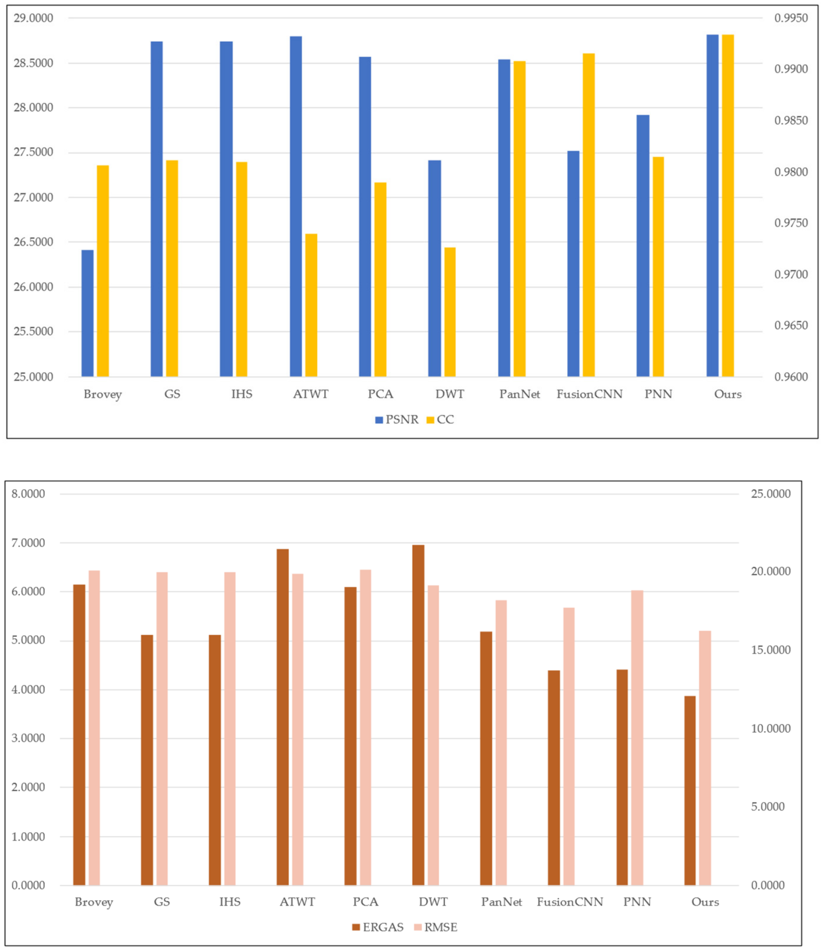
| Fusion Method | PSNR | ERGAS | RMSE | CC |
|---|---|---|---|---|
| Brovey | 26.4100 | 6.1519 | 20.1044 | 0.9806 |
| GS | 28.7420 | 5.1143 | 20.0054 | 0.9811 |
| IHS | 28.7369 | 5.1160 | 20.0105 | 0.9810 |
| ATWT | 28.8015 | 6.8793 | 19.9130 | 0.9740 |
| PCA | 28.5646 | 6.0954 | 20.1777 | 0.9790 |
| DWT | 27.4118 | 6.9636 | 19.1508 | 0.9726 |
| PanNet | 28.5425 | 5.1880 | 18.2084 | 0.9908 |
| FusionCNN | 27.5199 | 4.3925 | 17.7332 | 0.9916 |
| PNN | 27.9194 | 4.4152 | 18.8455 | 0.9815 |
| Ours | 28.8136 | 3.8734 | 16.2711 | 0.9934 |
| Fusion Method | PSNR | ERGAS | RMSE | CC |
|---|---|---|---|---|
| Brovey | 31.9912 | 5.4425 | 27.3828 | 0.8618 |
| GS | 32.5129 | 5.2646 | 26.6783 | 0.8663 |
| IHS | 32.4823 | 5.2995 | 26.7186 | 0.8664 |
| ATWT | 35.8258 | 2.5560 | 12.9034 | 0.9648 |
| PCA | 31.9379 | 5.4145 | 27.4569 | 0.9657 |
| DWT | 34.3709 | 2.6027 | 13.1378 | 0.9635 |
| PanNet | 37.4864 | 3.1304 | 14.7722 | 0.9653 |
| FusionCNN | 37.6786 | 2.5543 | 12.8365 | 0.9804 |
| PNN | 37.5268 | 3.1121 | 14.8292 | 0.9671 |
| Ours | 38.3922 | 2.5403 | 12.7677 | 0.9809 |
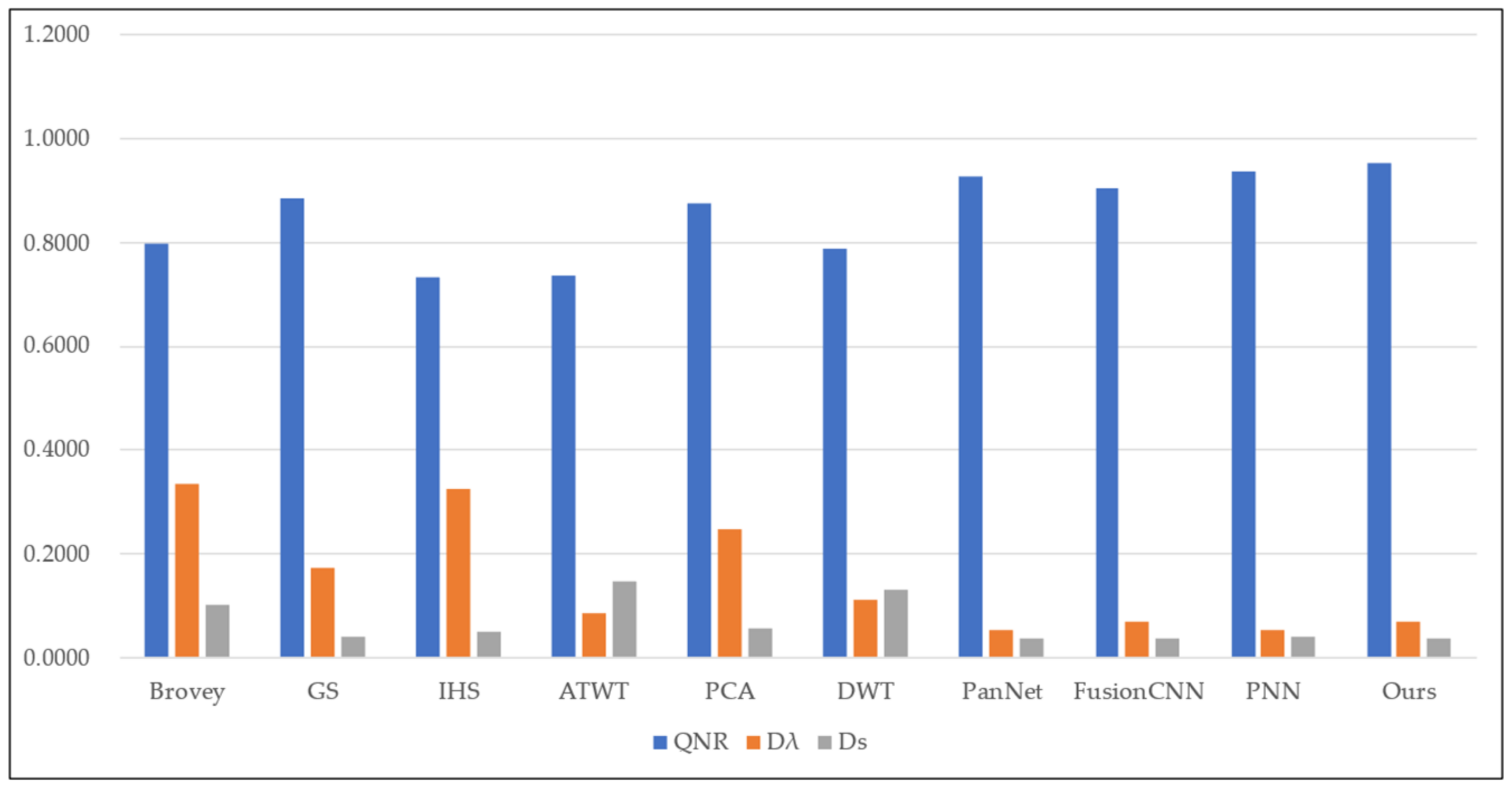
| Fusion Method | QNR | ||
|---|---|---|---|
| Brovey | 0.7979 | 0.3343 | 0.1022 |
| GS | 0.8863 | 0.1717 | 0.0407 |
| IHS | 0.7316 | 0.3245 | 0.0503 |
| ATWT | 0.7375 | 0.0843 | 0.1465 |
| PCA | 0.8767 | 0.2464 | 0.0562 |
| DWT | 0.7886 | 0.1114 | 0.1302 |
| PanNet | 0.9273 | 0.0522 | 0.0373 |
| FusionCNN | 0.9041 | 0.0679 | 0.0356 |
| PNN | 0.9368 | 0.0530 | 0.0396 |
| Ours | 0.9528 | 0.0696 | 0.0348 |
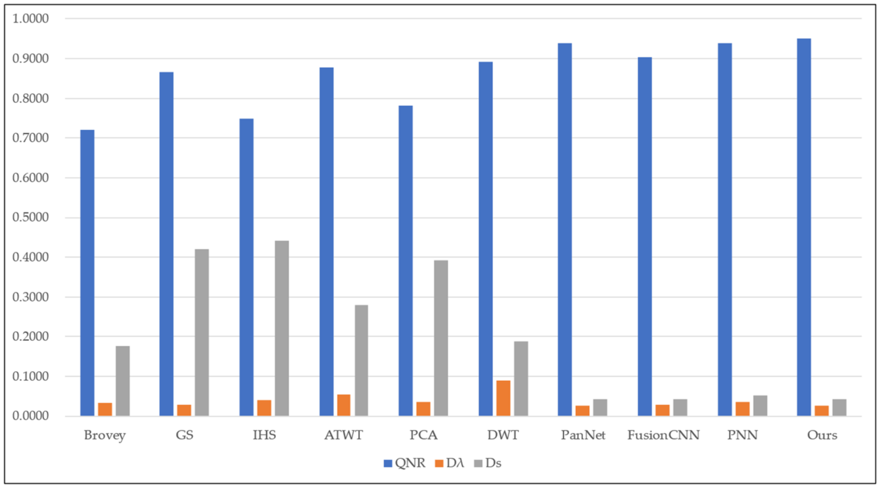
| Fusion Method | QNR | ||
|---|---|---|---|
| Brovey | 0.7200 | 0.0323 | 0.1754 |
| GS | 0.8673 | 0.0278 | 0.4198 |
| IHS | 0.7481 | 0.0399 | 0.4409 |
| ATWT | 0.8777 | 0.0531 | 0.2787 |
| PCA | 0.7813 | 0.0365 | 0.3911 |
| DWT | 0.8917 | 0.0896 | 0.1870 |
| PanNet | 0.9388 | 0.0253 | 0.0424 |
| FusionCNN | 0.9041 | 0.0273 | 0.0427 |
| PNN | 0.9385 | 0.0343 | 0.0528 |
| Ours | 0.9515 | 0.0262 | 0.0418 |
Publisher’s Note: MDPI stays neutral with regard to jurisdictional claims in published maps and institutional affiliations. |
© 2022 by the authors. Licensee MDPI, Basel, Switzerland. This article is an open access article distributed under the terms and conditions of the Creative Commons Attribution (CC BY) license (https://creativecommons.org/licenses/by/4.0/).
Share and Cite
Jia, B.; Xu, J.; Xing, H.; Wu, P. Remote Sensing Image Fusion Based on Morphological Convolutional Neural Networks with Information Entropy for Optimal Scale. Sensors 2022, 22, 7339. https://doi.org/10.3390/s22197339
Jia B, Xu J, Xing H, Wu P. Remote Sensing Image Fusion Based on Morphological Convolutional Neural Networks with Information Entropy for Optimal Scale. Sensors. 2022; 22(19):7339. https://doi.org/10.3390/s22197339
Chicago/Turabian StyleJia, Bairu, Jindong Xu, Haihua Xing, and Peng Wu. 2022. "Remote Sensing Image Fusion Based on Morphological Convolutional Neural Networks with Information Entropy for Optimal Scale" Sensors 22, no. 19: 7339. https://doi.org/10.3390/s22197339