
Spatial Interpolation of Gravimetric Soil Moisture Using EM38-mk Induction and Ensemble Machine Learning (Case Study from Dry Steppe Zone in Volgograd Region)


Abstract
:1. Introduction
2. Materials and Methods
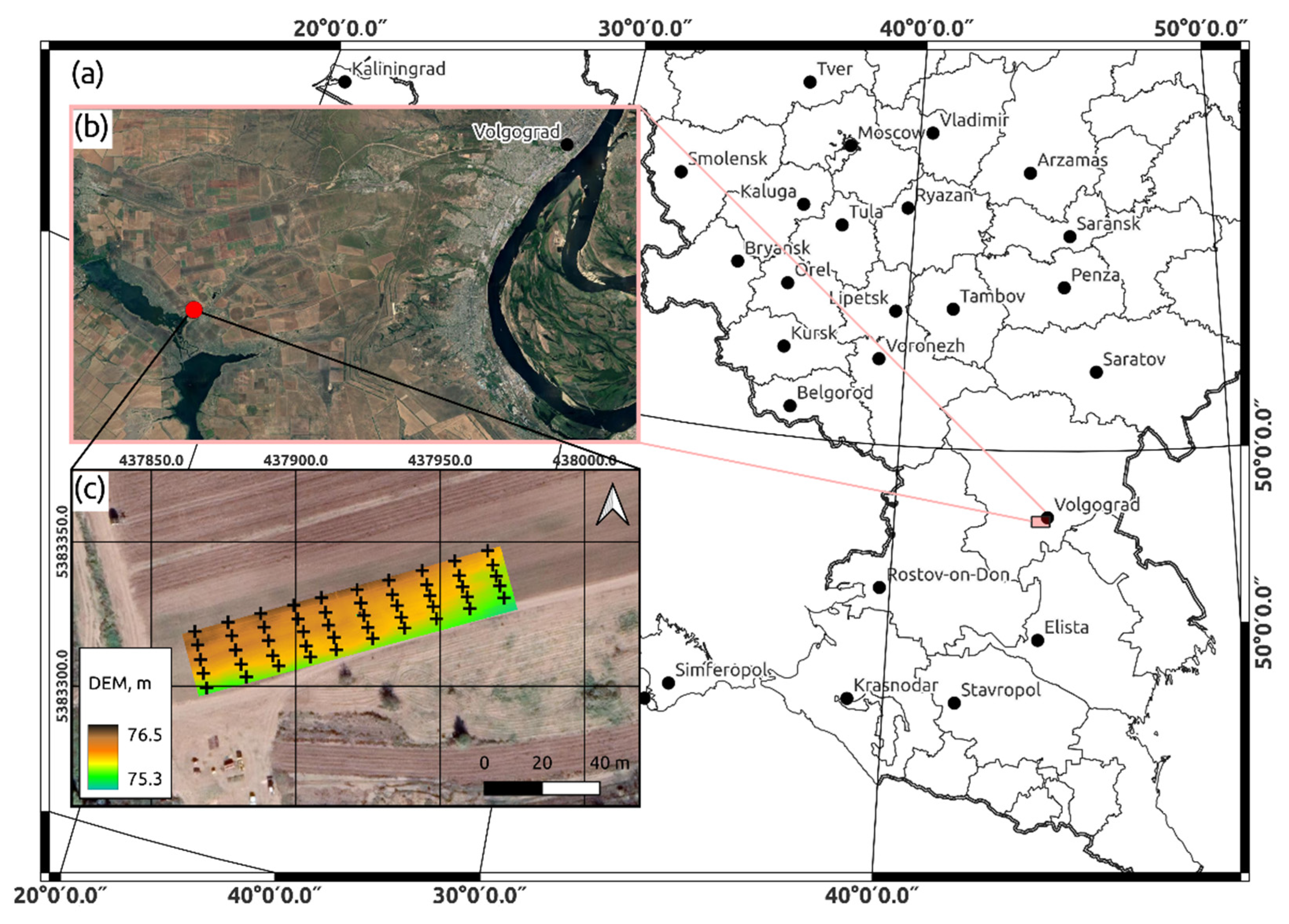
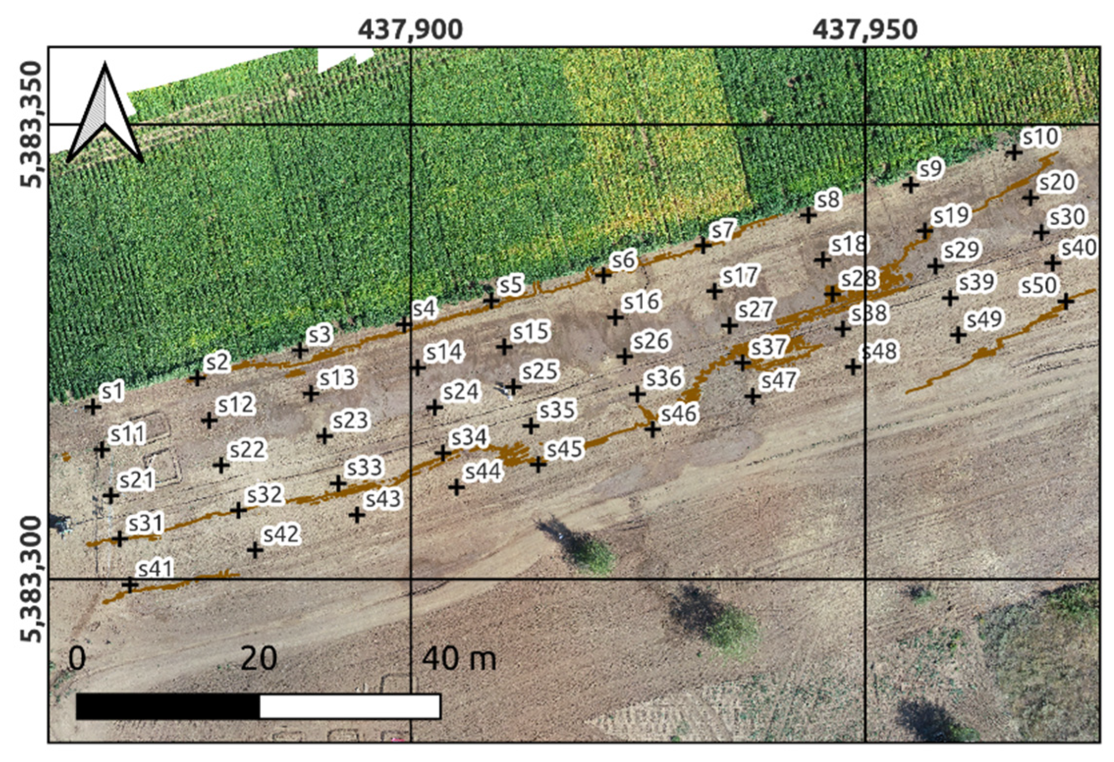
2.1. Study Area
- (a)
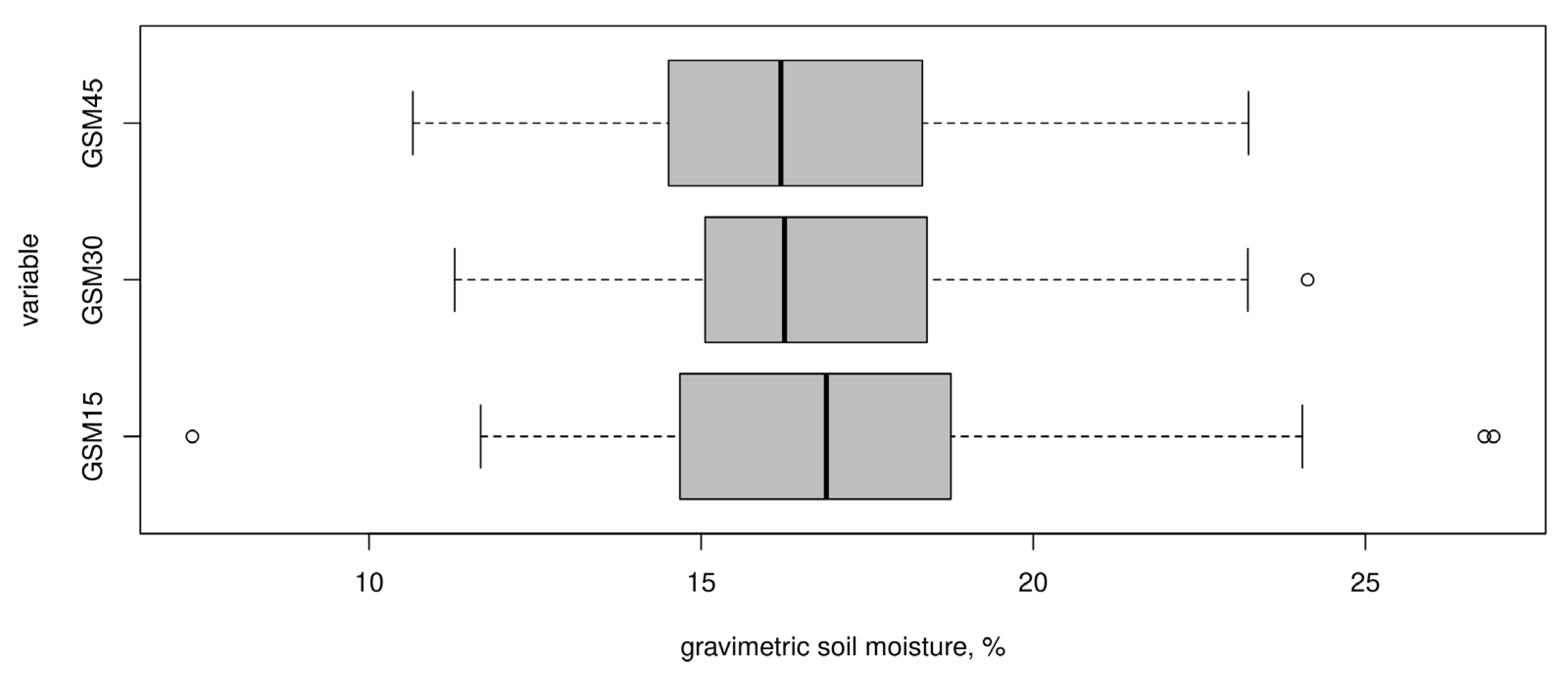
- the moisture of soil samples and the coordinates of sampling places;
- (b)
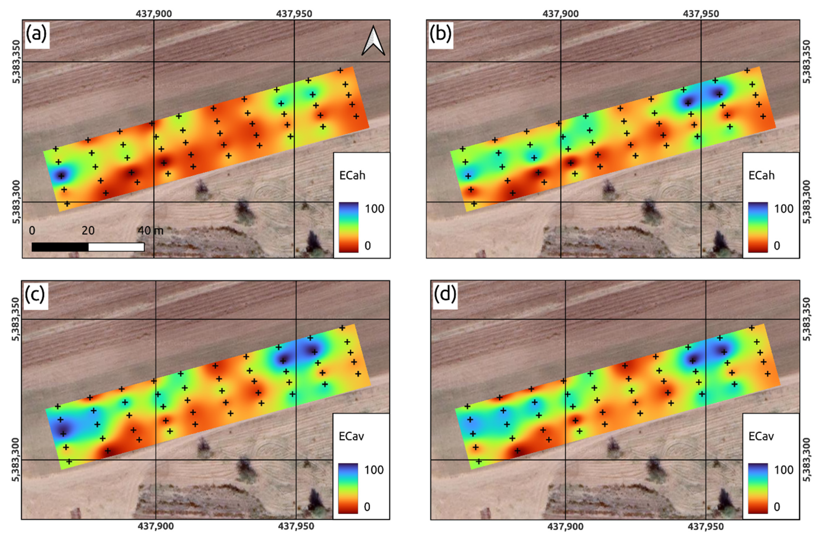
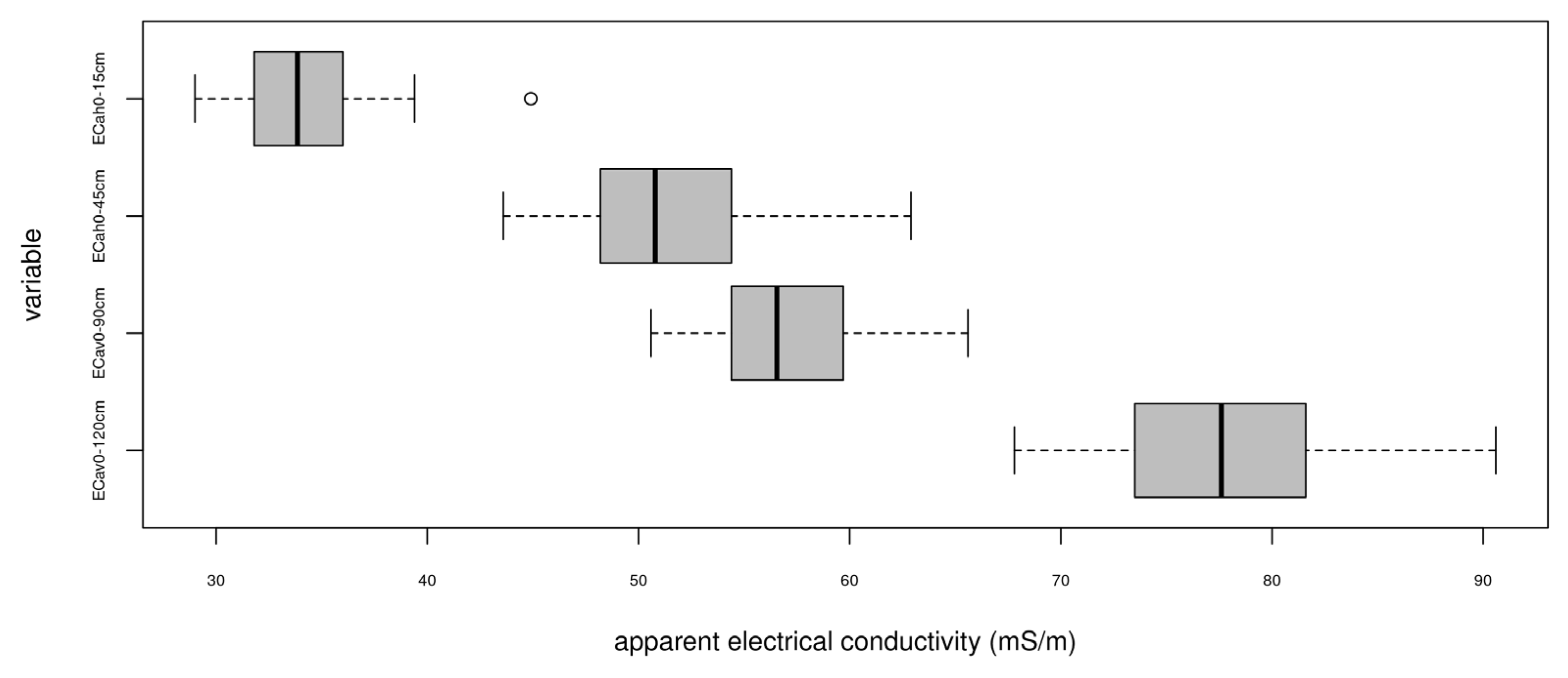
- proximal soil sensing obtained with the EM38-mk Electomagnetic Induction Meter;
- (c)
- the characteristics of a digital elevation model (DEM) calculated from the results of stereophotogrammetric survey from a UAV;
- (d)
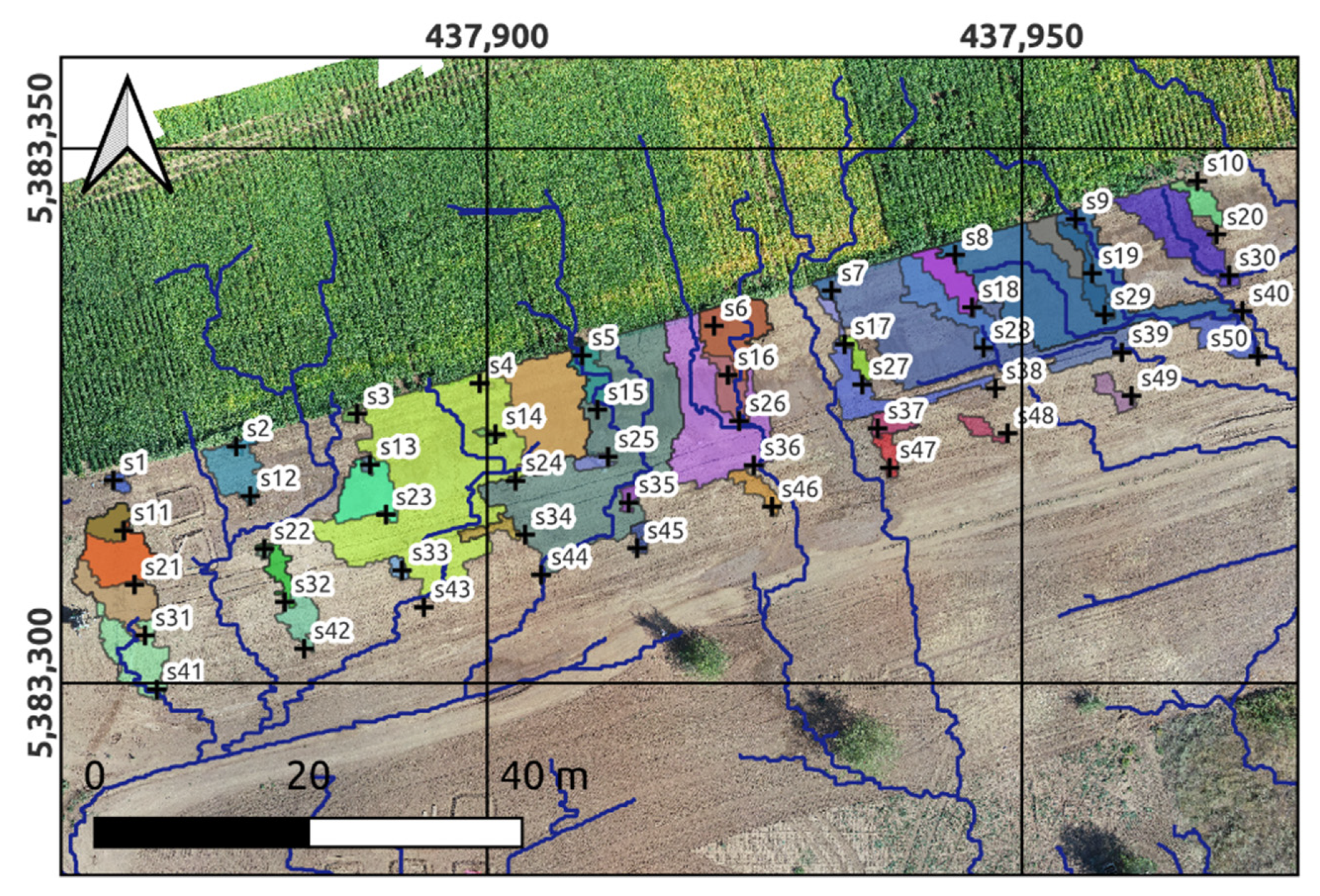
- the characteristics of the relative position of the elements of the hydrological network.
2.2. Methods
2.2.1. Input Data
2.2.2. Modelling Workflow
- the preparation of initial data;
- the intersection (overlay) of the existing observation points and the values of independent variables at these points (the creation of a regression matrix);
- modeling with the stepwise inclusion of independent variables using an ensemble machine learning methods and spatial cross-validation;
- the assessment of the accuracy of the obtained models;
- the spatial prediction of gravimetric soil moisture for each element (pixel) of the raster (prediction on new data).
2.2.3. Ensemble Machine Learning
- Set up the ensemble.
- (a)
- Specify a list of L base (null) algorithms (with a specific set of model parameters);
- (b)
- Specify a metalearning algorithm.
- Train the ensemble.
- (a)
- Train each of the L base algorithms using the training set;
- (b)
- Perform k-fold cross-validation on each of these learners and collect the cross-validated predicted values from each of the L algorithms;
- (c)
- The N cross-validated predicted values from each of the L algorithms can be combined to form a new N × L matrix. This matrix, along with the original response vector, is called the “level-one” data. (N = number of rows in the training set);
- (d)
- Train the metalearning algorithm on the level-one data. The “ensemble model” consists of the L base learning models and the metalearning model, which can then be used to generate predictions on a test set.
- Predict using new data.
- (a)
- To generate ensemble predictions, first generate predictions from the base learners;
- (b)
- Feed those predictions into the metalearner to generate the ensemble prediction.
- the derivation of geographical distances (Euclidean distances to sampling sites, i.e., distances from observation sites. For each observation point, one buffer distance map is generated);
- the conversion of grids to principal components (to remove the multicollinearity effect of some independent variables);
- the automated filling of gaps in gridded data;
- the automated fitting of variogram and the determination of spatial auto-correlation structure;
- spatial overlay;
- model training using spatial cross-validation;
- model stacking, i.e., the fitting of the final EML.
2.2.4. Model Evaluation
3. Results
3.1. Exploratory Data Analysis of Soil and Proximal Data at Sampling Sites
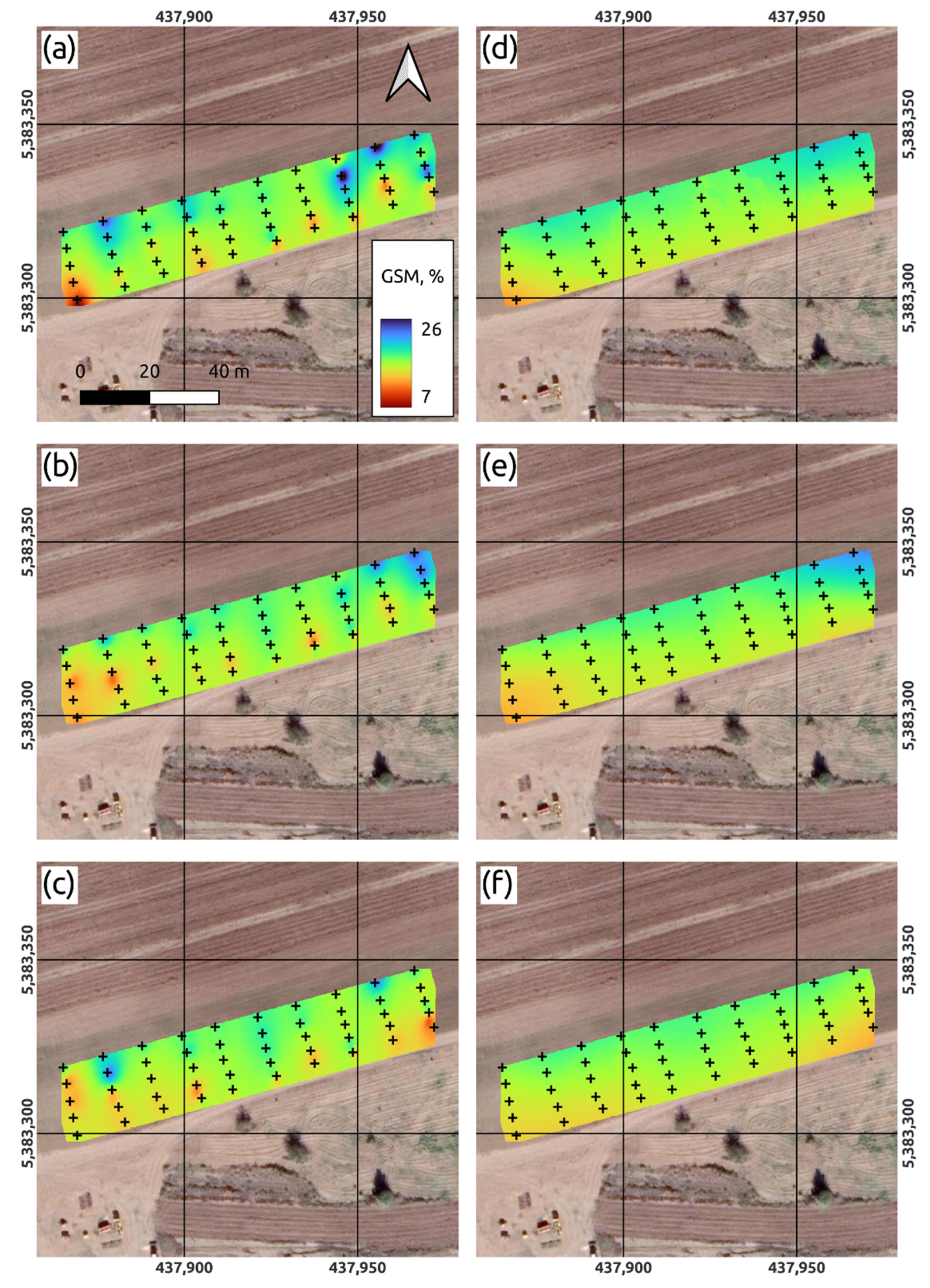
3.2. Evaluation of Model Performance
4. Discussion
5. Conclusions
Author Contributions
Funding
Institutional Review Board Statement
Informed Consent Statement
Data Availability Statement
Acknowledgments
Conflicts of Interest
References
- GCOS. The Global Climate Observing System 2021: The GCOS Status Report; GCOS: Geneva, Switzerland, 2021; Volume 240. [Google Scholar]
- Zinchenko, E.V.; Gorokhova, I.N.; Kruglyakova, N.G.; Khitrov, N.B. Modern State of Irrigated Soils at the South of the Volga Upland. Dokuchaev Soil Bull. 2020, 104, 68–109. [Google Scholar] [CrossRef]
- Khitrov, N.B.; Gorokhova, I.N.; Pankova, Y.I. Remote Sensing of the Carbonate Content in Irrigated Soils of the Dry Steppe Zone in Volgograd Oblast. Eurasian Soil Sci. 2021, 54, 827–842. [Google Scholar] [CrossRef]
- Poggio, L.; de Sousa, L.M.; Batjes, N.H.; Heuvelink, G.B.M.; Kempen, B.; Ribeiro, E.; Rossiter, D. SoilGrids 2.0: Producing Soil Information for the Globe with Quantified Spatial Uncertainty. SOIL 2021, 7, 217–240. [Google Scholar] [CrossRef]
- Arrouays, D.; McKenzie, N.; Hempel, J.; Richer de Forges, A.; McBratney, A.B. Global Soil Map: Basis of the Global Spatial Soil Information System; CRC Press/Balkema: Boca Raton, FL, USA, 2014. [Google Scholar]
- Zeyliger, A.M.; Ermolaeva, O.S. Water Stress Regime of Irrigated Crops Based on Remote Sensing and Ground-Based Data. Agronomy 2021, 11, 1117. [Google Scholar] [CrossRef]
- Savin, I.Y.; Zhogolev, A.V.; Prudnikova, E.Y. Modern Trends and Problems of Soil Mapping. Eurasian Soil Sci. 2019, 52, 471–480. [Google Scholar] [CrossRef]
- McBratney, A.B.; Mendonça Santos, M.L.; Minasny, B. On Digital Soil Mapping. Geoderma 2003, 117, 3–52. [Google Scholar] [CrossRef]
- Hengl, T.; MacMillan, R.A. Predictive Soil Mapping with R; OpenGeoHub Foundation: Wageningen, The Netherlands, 2019; p. 370. [Google Scholar]
- Hartemink, A.E.; Minasny, B. Towards Digital Soil Morphometrics. Geoderma 2014, 230–231, 305–317. [Google Scholar] [CrossRef]
- Zhao, D.; Wang, J.; Zhao, X.; Triantafilis, J. Clay Content Mapping and Uncertainty Estimation Using Weighted Model Averaging. CATENA 2022, 209, 105791. [Google Scholar] [CrossRef]
- Arshad, M.; Zhao, D.; Zare, E.; Sefton, M.; Triantafilis, J. Proximally Sensed Digital Data Library to Predict Topsoil Clay across Multiple Sugarcane Fields of Australia: Applicability of Local and Universal Support Vector Machine. CATENA 2021, 196, 104934. [Google Scholar] [CrossRef]
- Arshad, M.; Li, N.; Bella, L.D.; Triantafilis, J. Field-scale Digital Soil Mapping of Clay: Combining Different Proximal Sensed Data and Comparing Various Statistical Models. Soil Sci. Soc. Am. J. 2020, 84, 314–330. [Google Scholar] [CrossRef]
- Zhao, D.; Li, N.; Zare, E.; Wang, J.; Triantafilis, J. Mapping Cation Exchange Capacity Using a Quasi-3d Joint Inversion of EM38 and EM31 Data. Soil Tillage Res. 2020, 200, 104618. [Google Scholar] [CrossRef]
- Abdu, H.; Robinson, D.A.; Seyfried, M.; Jones, S.B. Geophysical Imaging of Watershed Subsurface Patterns and Prediction of Soil Texture and Water Holding Capacity. Water Resour. Res. 2008, 44, W00D18. [Google Scholar] [CrossRef]
- Cardoso, R.; Dias, A.S. Study of the Electrical Resistivity of Compacted Kaolin Based on Water Potential. Eng. Geol. 2017, 226, 1–11. [Google Scholar] [CrossRef]
- Farzamian, M.; Monteiro Santos, F.A.; Khalil, M.A. Application of EM38 and ERT Methods in Estimation of Saturated Hydraulic Conductivity in Unsaturated Soil. J. Appl. Geophys. 2015, 112, 175–189. [Google Scholar] [CrossRef]
- Khongnawang, T.; Zare, E.; Srihabun, P.; Khunthong, I.; Triantafilis, J. Digital Soil Mapping of Soil Salinity Using EM38 and Quasi-3d Modelling Software (EM4Soil). Soil Use Manag. 2022, 38, 277–291. [Google Scholar] [CrossRef]
- Khongnawang, T.; Zare, E.; Srihabun, P.; Triantafilis, J. Comparing Electromagnetic Induction Instruments to Map Soil Salinity in Two-Dimensional Cross-Sections along the Kham-Rean Canal Using EM Inversion Software. Geoderma 2020, 377, 114611. [Google Scholar] [CrossRef]
- Narjary, B.; Meena, M.D.; Kumar, S.; Kamra, S.K.; Sharma, D.K.; Triantafilis, J. Digital Mapping of Soil Salinity at Various Depths Using an EM38. Soil Use Manag. 2019, 35, 232–244. [Google Scholar] [CrossRef]
- Chinilin, A.V.; Savin, I.Y. The Large Scale Digital Mapping of Soil Organic Carbon Using Machine Learning Algorithms. Dokuchaev Soil Bull. 2018, 91, 46–62. [Google Scholar] [CrossRef]
- Suleymanov, A.; Abakumov, E.; Suleymanov, R.; Gabbasova, I.; Komissarov, M. The Soil Nutrient Digital Mapping for Precision Agriculture Cases in the Trans-Ural Steppe Zone of Russia Using Topographic Attributes. ISPRS Int. J. Geo-Inf. 2021, 10, 243. [Google Scholar] [CrossRef]
- Hengl, T.; Miller, M.A.E.; Križan, J.; Shepherd, K.D.; Sila, A.; Kilibarda, M.; Antonijević, O.; Glušica, L.; Dobermann, A.; Haefele, S.M.; et al. African Soil Properties and Nutrients Mapped at 30 m Spatial Resolution Using Two-Scale Ensemble Machine Learning. Sci. Rep. 2021, 11, 6130. [Google Scholar] [CrossRef]
- Sothe, C.; Gonsamo, A.; Arabian, J.; Snider, J. Large Scale Mapping of Soil Organic Carbon Concentration with 3D Machine Learning and Satellite Observations. Geoderma 2022, 405, 115402. [Google Scholar] [CrossRef]
- Behrens, T.; Schmidt, K.; Viscarra Rossel, R.A.; Gries, P.; Scholten, T.; MacMillan, R.A. Spatial Modelling with Euclidean Distance Fields and Machine Learning. Eur. J. Soil Sci. 2018, 69, 757–770. [Google Scholar] [CrossRef]
- Hengl, T.; Nussbaum, M.; Wright, M.N.; Heuvelink, G.B.M.; Gräler, B. Random Forest as a Generic Framework for Predictive Modeling of Spatial and Spatio-Temporal Variables. PeerJ 2018, 6, e5518. [Google Scholar] [CrossRef] [PubMed]
- Møller, A.B.; Beucher, A.M.; Pouladi, N.; Greve, M.H. Oblique Geographic Coordinates as Covariates for Digital Soil Mapping. SOIL 2020, 6, 269–289. [Google Scholar] [CrossRef]
- Sekulić, A.; Kilibarda, M.; Heuvelink, G.B.M.; Nikolić, M.; Bajat, B. Random Forest Spatial Interpolation. Remote Sens. 2020, 12, 1687. [Google Scholar] [CrossRef]
- FAO. Guidelines for Soil Description 4th Edn. Food and Agriculture Organisation of the United Nations; INSPIRE: Rome, Italy, 2006; Volume 16. [Google Scholar]
- Zeyliger, A.M.; Tuluzakov, M.L. Jelektromagnitnyj induktometr dlja vertikal’nogo profilirovanija vlagozapasov pochvenno-gruntovoj tolshhi. Prirodoobustrojstvo 2013, 4, 36–40. [Google Scholar]
- Conrad, O.; Bechtel, B.; Bock, M.; Dietrich, H.; Fischer, E.; Gerlitz, L.; Wehberg, J.; Wichmann, V.; Böhner, J. System for Automated Geoscientific Analyses (SAGA) v. 2.1.4. Geosci. Model Dev. 2015, 8, 1991–2007. [Google Scholar] [CrossRef]
- Breiman, L. Stacked Regressions. Mach. Learn. 1996, 24, 49–64. [Google Scholar] [CrossRef]
- van der Laan, M.J.; Polley, E.C.; Hubbard, A.E. Super Learner. Stat. Appl. Genet. Mol. Biol. 2007, 6, 25. [Google Scholar] [CrossRef]
- Wolpert, D.H. Stacked Generalization. Neural Netw. 1992, 5, 241–259. [Google Scholar] [CrossRef]
- Li, X.; Luo, J.; Jin, X.; He, Q.; Niu, Y. Improving Soil Thickness Estimations Based on Multiple Environmental Variables with Stacking Ensemble Methods. Remote Sens. 2020, 12, 3609. [Google Scholar] [CrossRef]
- Song, X.-D.; Wu, H.-Y.; Ju, B.; Liu, F.; Yang, F.; Li, D.-C.; Zhao, Y.-G.; Yang, J.-L.; Zhang, G.-L. Pedoclimatic Zone-Based Three-Dimensional Soil Organic Carbon Mapping in China. Geoderma 2020, 363, 114145. [Google Scholar] [CrossRef]
- Taghizadeh-Mehrjardi, R.; Hamzehpour, N.; Hassanzadeh, M.; Heung, B.; Ghebleh Goydaragh, M.; Schmidt, K.; Scholten, T. Enhancing the Accuracy of Machine Learning Models Using the Super Learner Technique in Digital Soil Mapping. Geoderma 2021, 399, 115108. [Google Scholar] [CrossRef]
- R Core Development Team. R: A Language and Environment for Statistical Computing; R Foundation for Statistical Computing: Vienna, Austria, 2016. [Google Scholar]
- Brenning, A. Spatial Prediction Models for Landslide Hazards: Review, Comparison and Evaluation. Nat. Hazards Earth Syst. Sci. 2005, 5, 853–862. [Google Scholar] [CrossRef]
- Mello, D.C.D.; Veloso, G.V.; Lana, M.G.D.; Mello, F.A.D.O.; Poppiel, R.R.; Cabrero, D.R.O.; Di Raimo, L.A.D.L.; Schaefer, C.E.G.R.; Filho, E.I.F.; Leite, E.P.; et al. A New Methodological Framework by Geophysical Sensors Combinations Associated with Machine Learning Algorithms to Understand Soil Attributes. Geosci. Model Dev. Discuss. 2022, 15, 1219–1246. [Google Scholar] [CrossRef]
- Saifuzzaman, M.; Adamchuk, V.; Biswas, A.; Rabe, N. High-Density Proximal Soil Sensing Data and Topographic Derivatives to Characterise Field Variability. Biosyst. Eng. 2021, 211, 19–34. [Google Scholar] [CrossRef]
- Aitkenhead, M.; Coull, M. Mapping Soil Profile Depth, Bulk Density and Carbon Stock in Scotland Using Remote Sensing and Spatial Covariates. Eur. J. Soil Sci. 2020, 71, 553–567. [Google Scholar] [CrossRef]
- Roudier, P.; Burge, O.R.; Richardson, S.J.; McCarthy, J.K.; Grealish, G.J.; Ausseil, A.-G. National Scale 3D Mapping of Soil PH Using a Data Augmentation Approach. Remote Sens. 2020, 12, 2872. [Google Scholar] [CrossRef]
- Nketia, K.A.; Asabere, S.B.; Ramcharan, A.; Herbold, S.; Erasmi, S.; Sauer, D. Spatio-Temporal Mapping of Soil Water Storage in a Semi-Arid Landscape of Northern Ghana—A Multi-Tasked Ensemble Machine-Learning Approach. Geoderma 2022, 410, 115691. [Google Scholar] [CrossRef]
- Meyer, H.; Pebesma, E. Predicting into unknown space? Estimating the area of applicability of spatial prediction models. Methods Ecol. Evol. 2021, 12, 1620–1633. [Google Scholar] [CrossRef]


| 0–15 cm | 15–30 cm | 30–45 cm | |
|---|---|---|---|
| n | 50 | 50 | 50 |
| mean | 17.09 | 16.77 | 16.30 |
| sd | 3.70 | 2.81 | 2.61 |
| median | 16.88 | 16.25 | 16.20 |
| min | 7.34 | 11.29 | 10.66 |
| max | 26.93 | 24.13 | 23.24 |
| range | 19.59 | 12.84 | 12.58 |
| skewness | 0.44 | 0.41 | 0.27 |
| kurtosis | 0.87 | 0.22 | −0.02 |
| se | 0.52 | 0.40 | 0.37 |
| ECav 0–120 cm 1 | ECav 0–90 cm | ECah 0–45 cm | ECah 0–15 cm | |
|---|---|---|---|---|
| n | 50 | 50 | 50 | 50 |
| mean | 77.59 | 57.13 | 51.40 | 33.96 |
| sd | 5.47 | 3.66 | 4.37 | 2.84 |
| median | 77.6 | 56.55 | 50.80 | 33.85 |
| min | 67.8 | 50.60 | 43.60 | 29.00 |
| max | 90.6 | 65.60 | 62.90 | 44.90 |
| range | 22.8 | 15.00 | 19.30 | 15.90 |
| skewness | 0.29 | 0.49 | 0.47 | 1.09 |
| kurtosis | −0.62 | −0.46 | −0.04 | 2.59 |
| se | 0.77 | 0.51 | 0.61 | 0.40 |
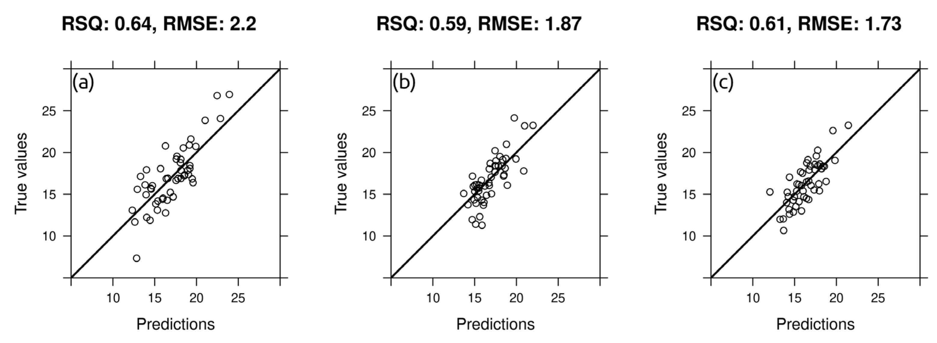
| Target Variables | Independent Variables | R2cv | RMSEcv |
|---|---|---|---|
| GSM 0–15 | DEM and derivatives | 0.28 | 3.29 |
| +buffer distances | 0.43 | 2.62 | |
| +ECa data | 0.57 | 2.50 | |
| PC 1 + buffer distances | 0.64 | 2.24 | |
| GSM 15–30 | DEM and derivatives | 0.31 | 3.13 |
| +buffer distances | 0.39 | 2.78 | |
| +ECa data | 0.53 | 2.19 | |
| PC + buffer distances | 0.59 | 1.87 | |
| GSM 30–45 | DEM and derivatives | 0.32 | 3.31 |
| +buffer distances | 0.39 | 2.74 | |
| +ECa data | 0.57 | 2.01 | |
| PC + buffer distances | 0.61 | 1.73 |
Publisher’s Note: MDPI stays neutral with regard to jurisdictional claims in published maps and institutional affiliations. |
© 2022 by the authors. Licensee MDPI, Basel, Switzerland. This article is an open access article distributed under the terms and conditions of the Creative Commons Attribution (CC BY) license (https://creativecommons.org/licenses/by/4.0/).
Share and Cite
Zeyliger, A.; Chinilin, A.; Ermolaeva, O. Spatial Interpolation of Gravimetric Soil Moisture Using EM38-mk Induction and Ensemble Machine Learning (Case Study from Dry Steppe Zone in Volgograd Region). Sensors 2022, 22, 6153. https://doi.org/10.3390/s22166153
Zeyliger A, Chinilin A, Ermolaeva O. Spatial Interpolation of Gravimetric Soil Moisture Using EM38-mk Induction and Ensemble Machine Learning (Case Study from Dry Steppe Zone in Volgograd Region). Sensors. 2022; 22(16):6153. https://doi.org/10.3390/s22166153
Chicago/Turabian StyleZeyliger, Anatoly, Andrey Chinilin, and Olga Ermolaeva. 2022. "Spatial Interpolation of Gravimetric Soil Moisture Using EM38-mk Induction and Ensemble Machine Learning (Case Study from Dry Steppe Zone in Volgograd Region)" Sensors 22, no. 16: 6153. https://doi.org/10.3390/s22166153