
Monitoring and Identification of Agricultural Crops through Multitemporal Analysis of Optical Images and Machine Learning Algorithms


 , ,
, ,
Abstract
:1. Introduction
1.1. Related Works
1.2. Contributions of This Work
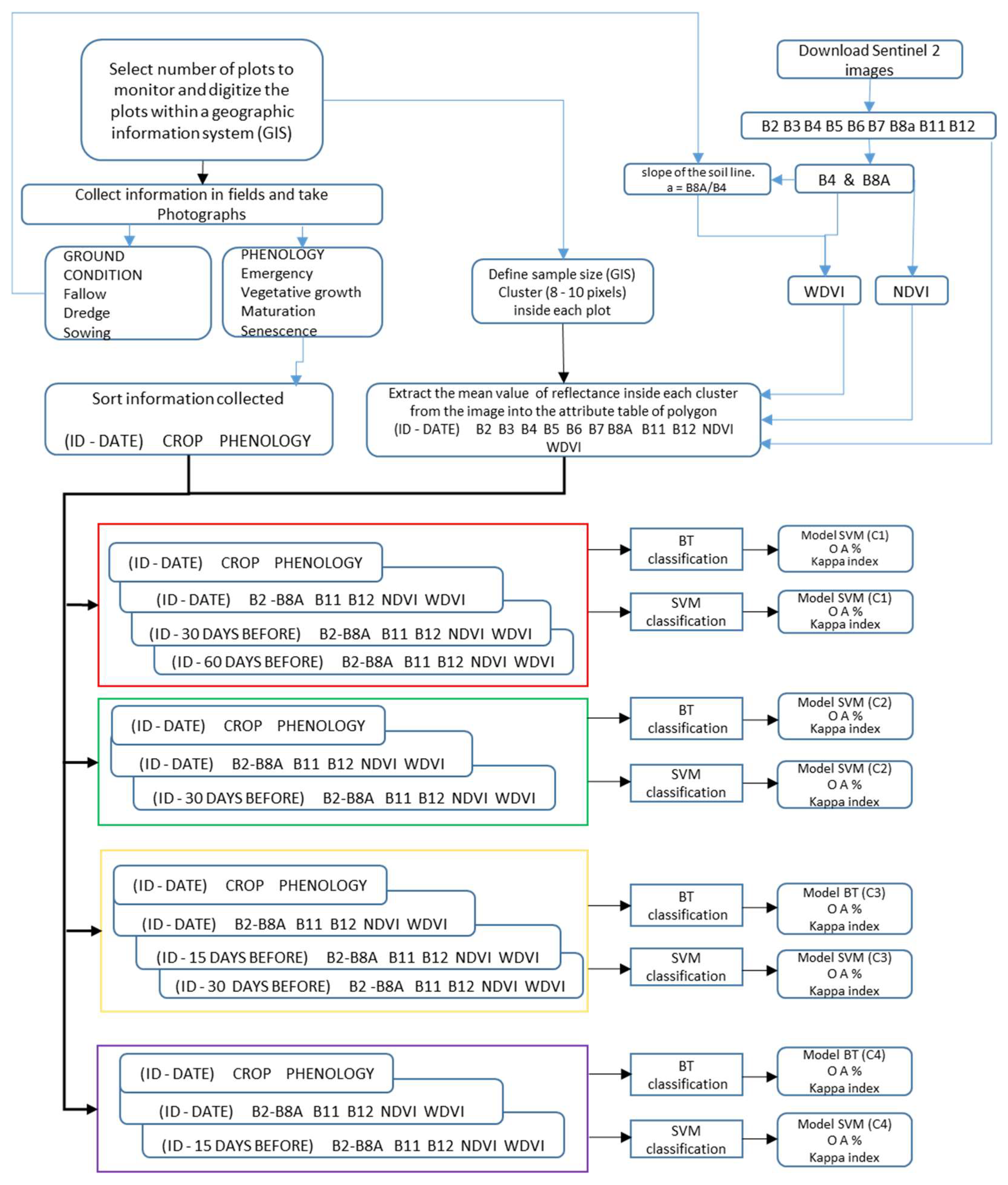
2. Materials and Methods
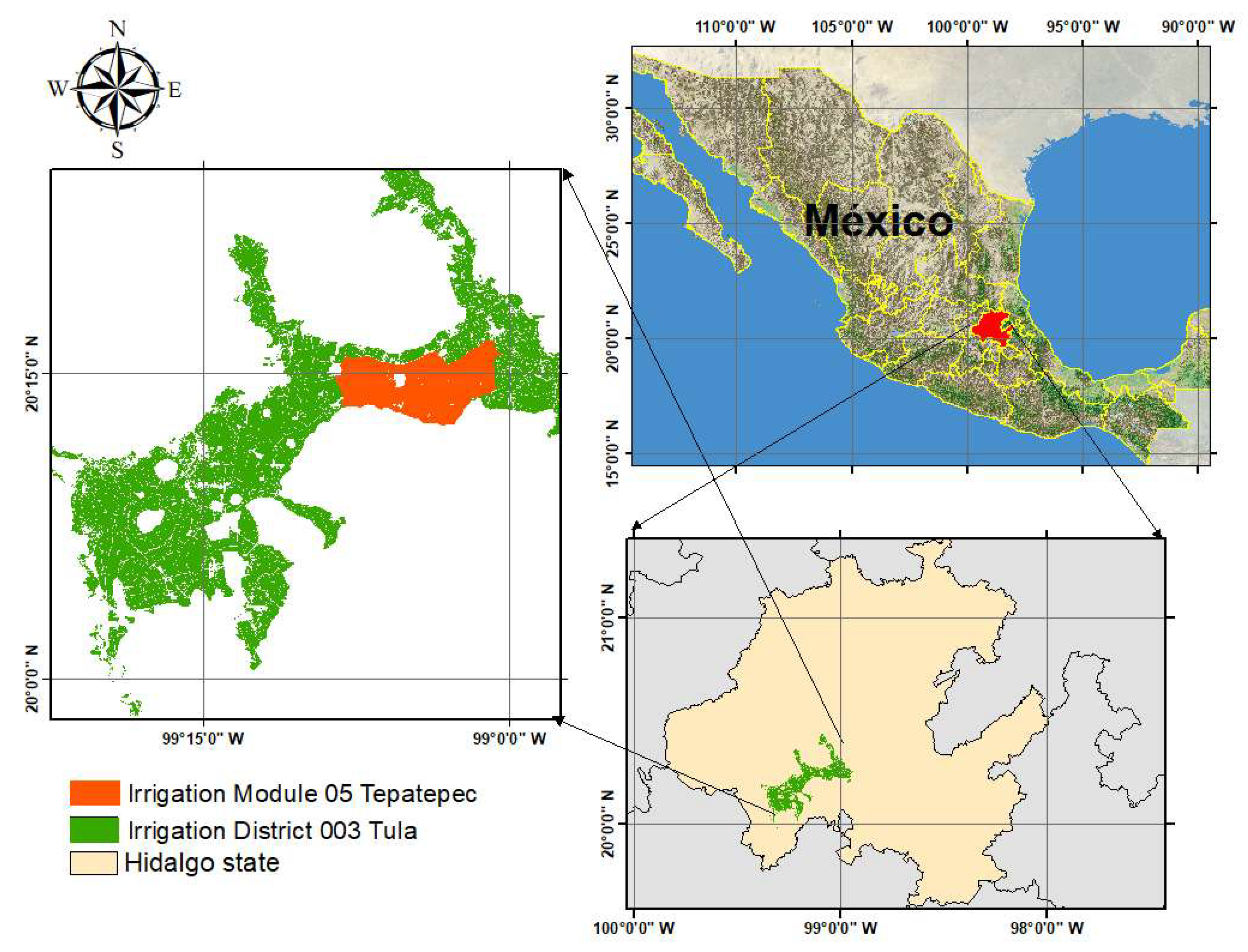
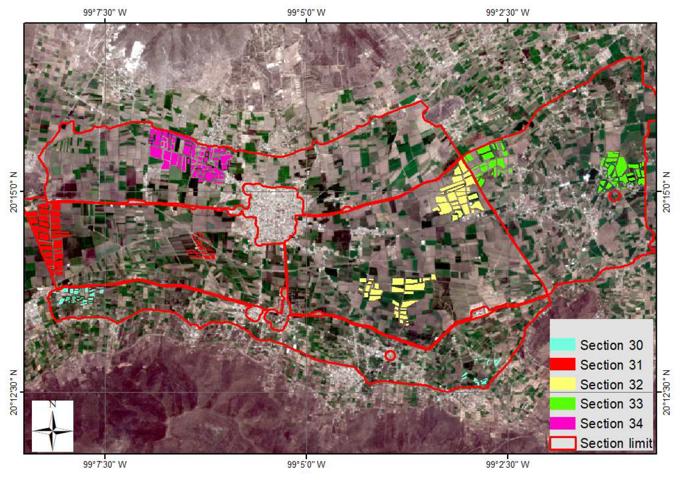
2.1. Study Area
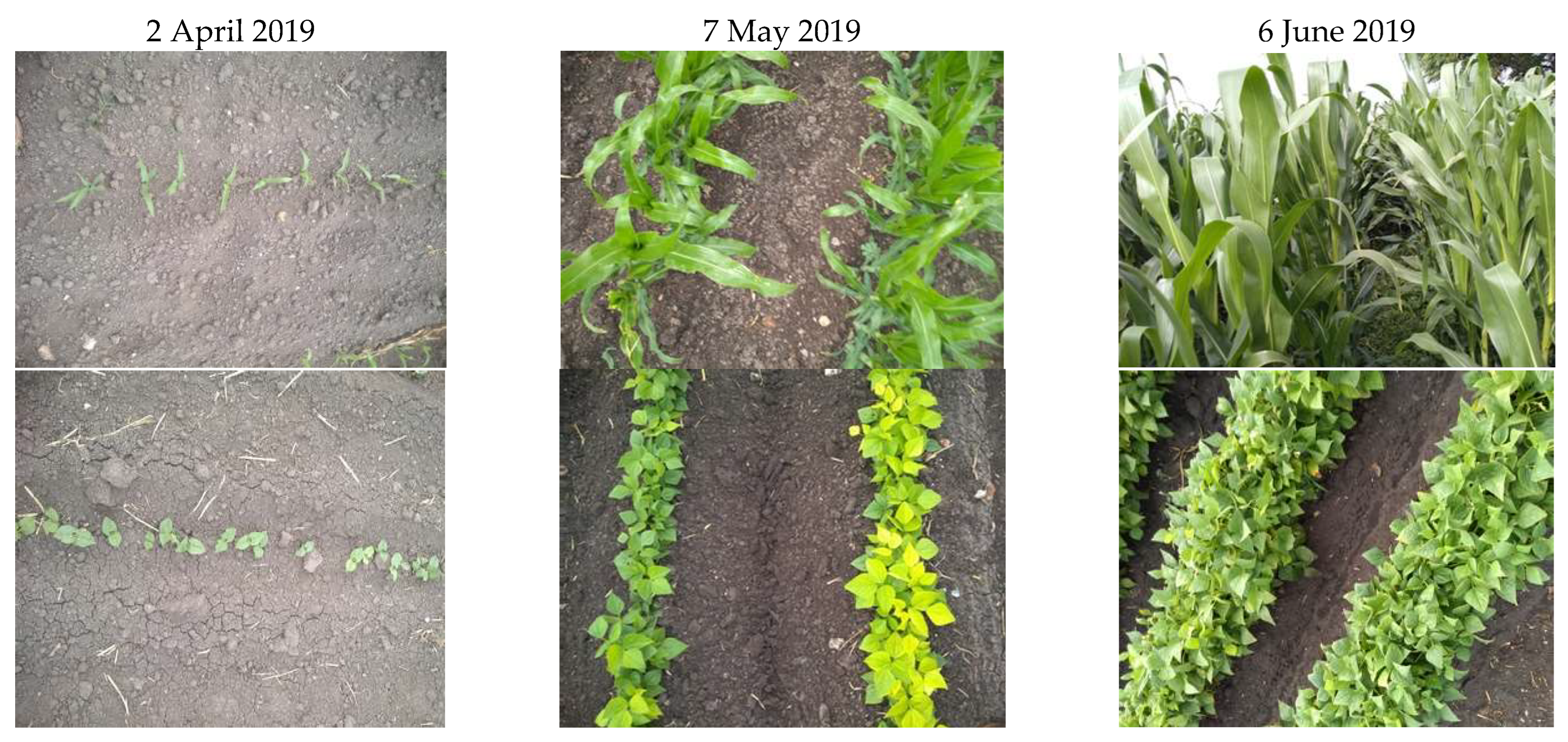
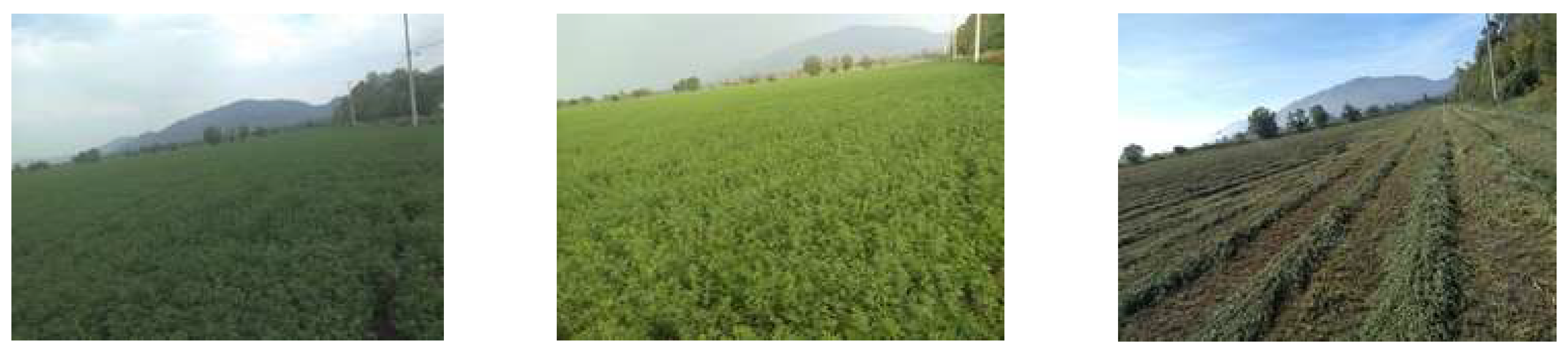
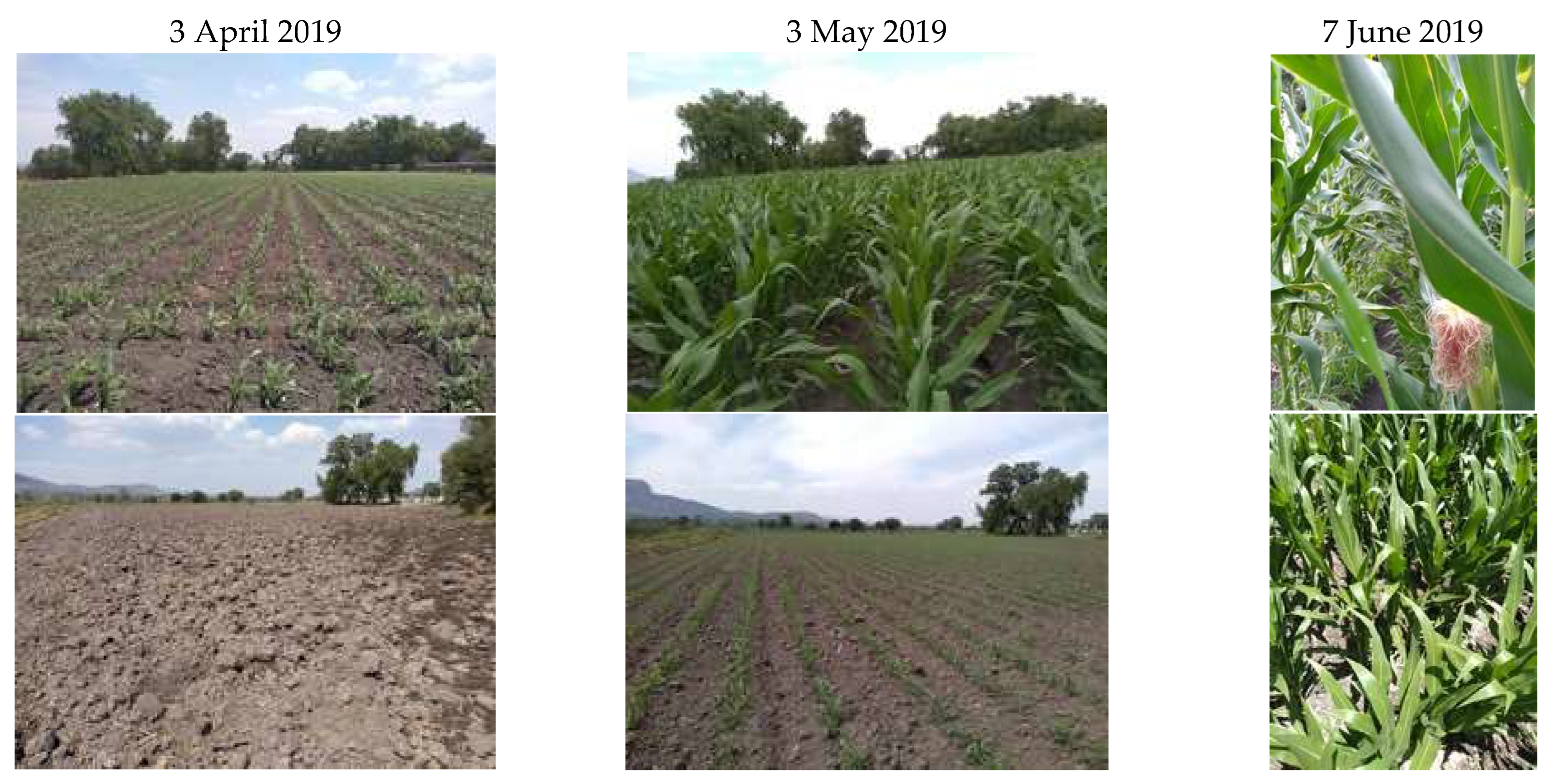
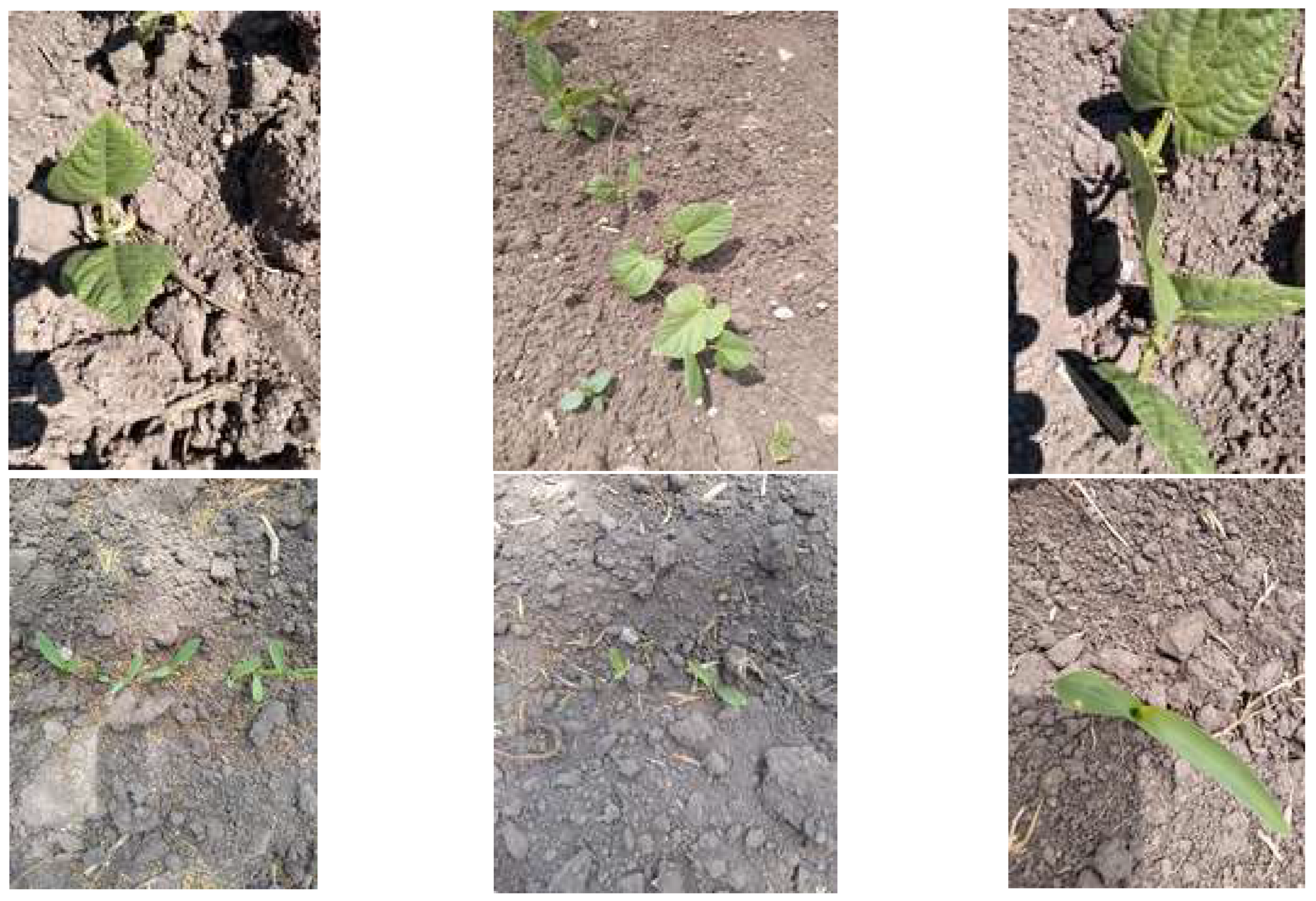
2.2. Crop Pattern
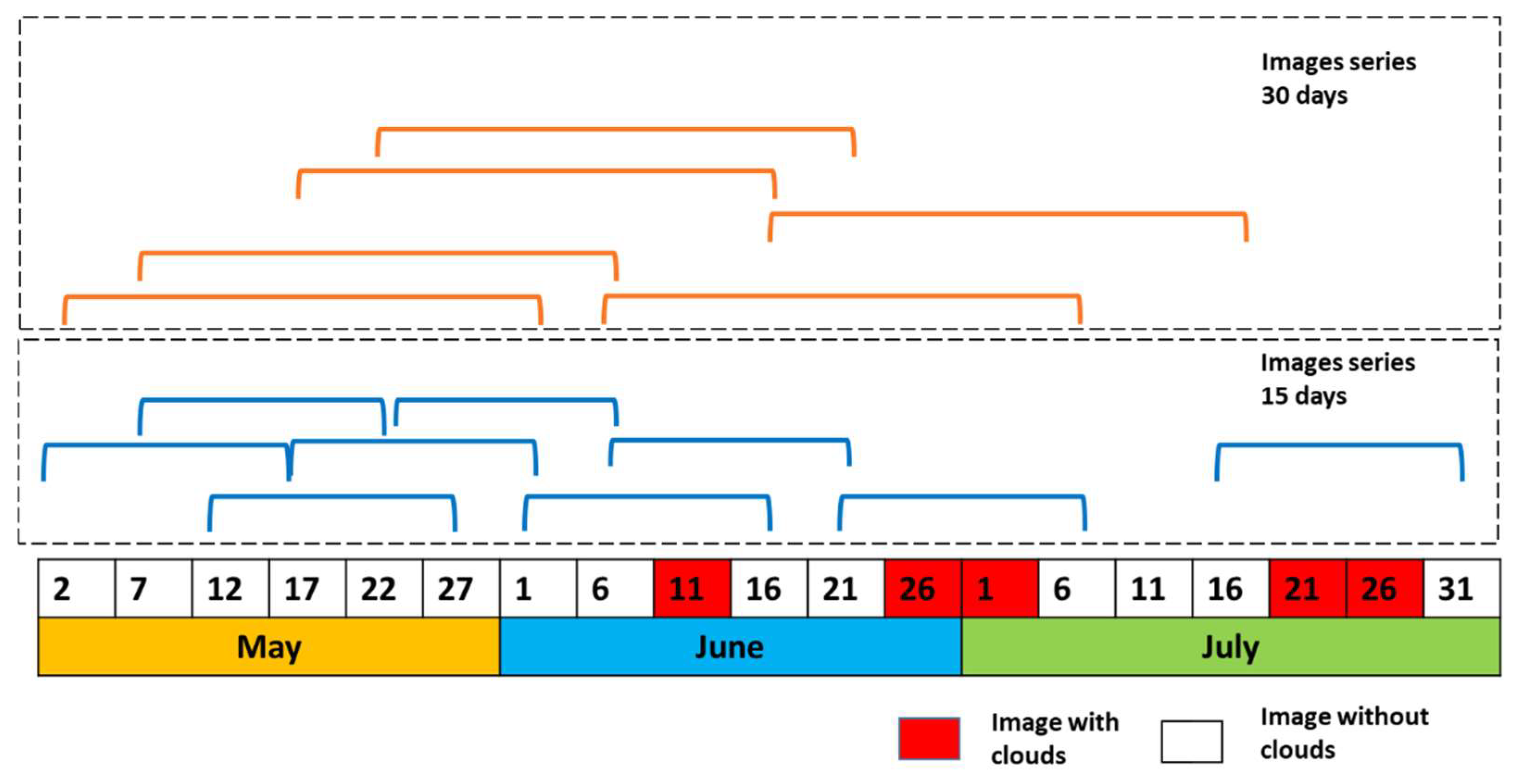
2.3. Data Input and Processing
- (a)
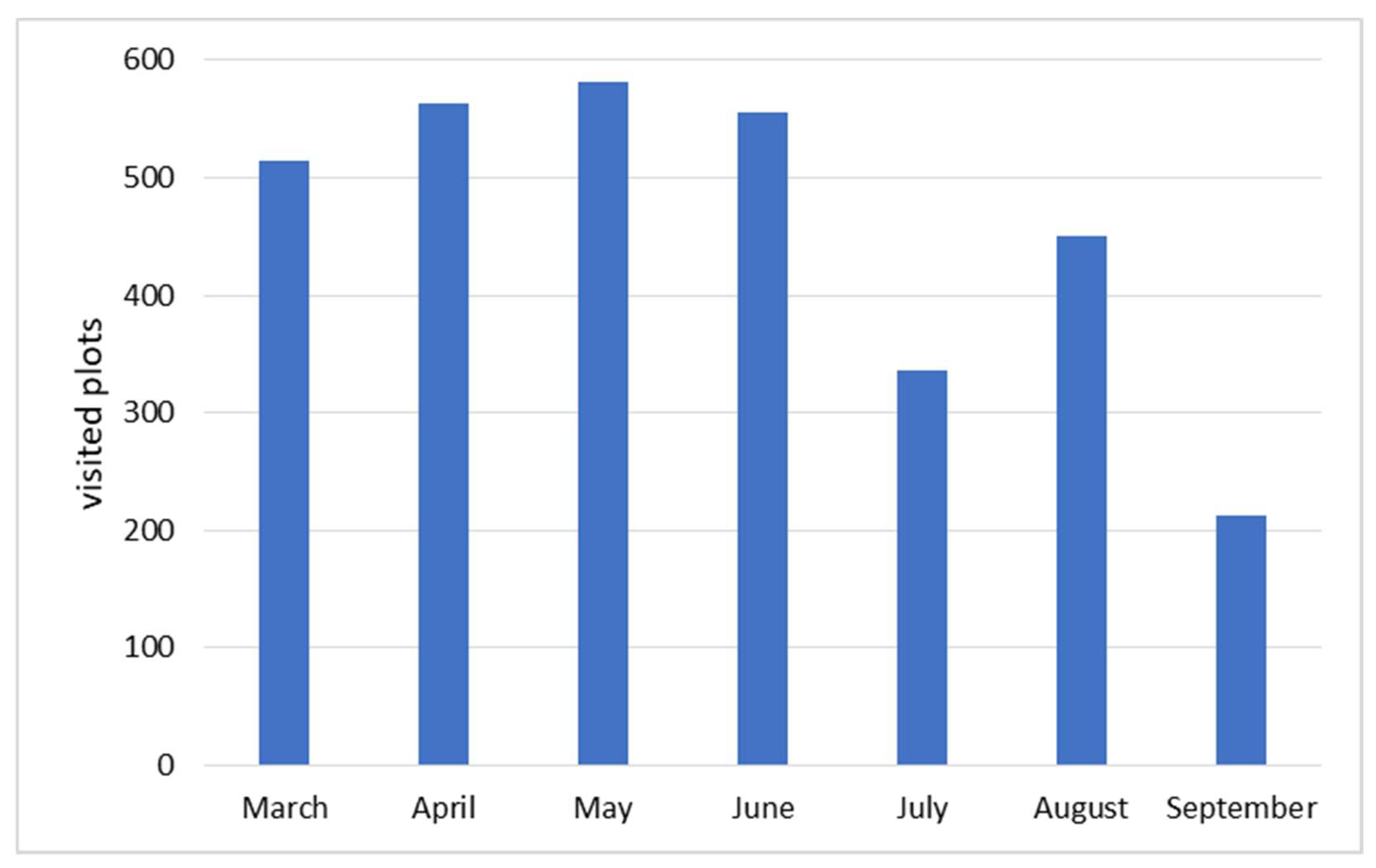
- Field survey data and frequency
- (b)
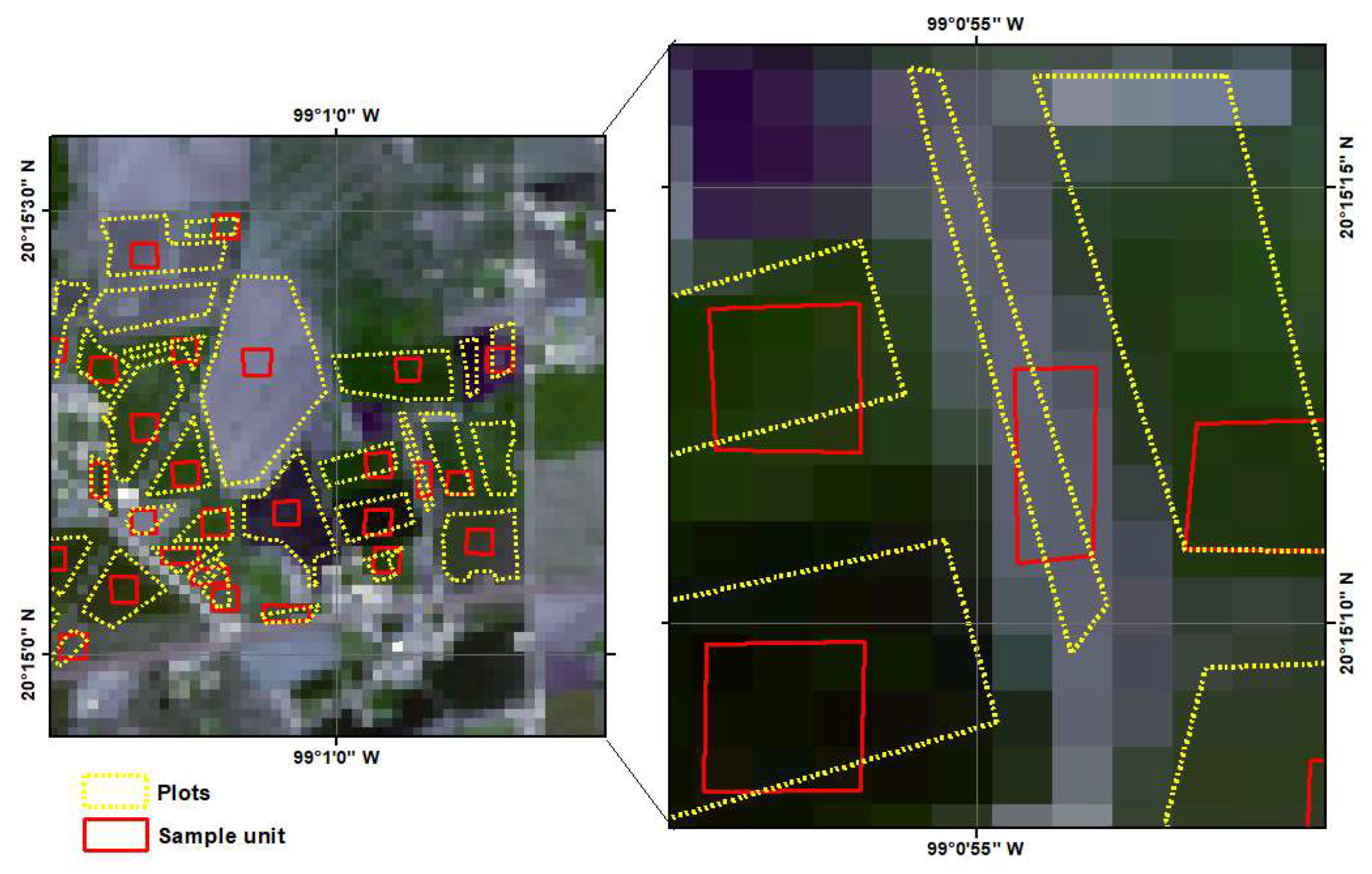
- Sampling unit taken from satellite images
- (c)
- Satellite images used
- (d)
- Characteristics used for training and validation
- (e)
- Database
- (f)
- Classification method and algorithm used
- (g)
- Validation of the models on same crop cycle
- (h)
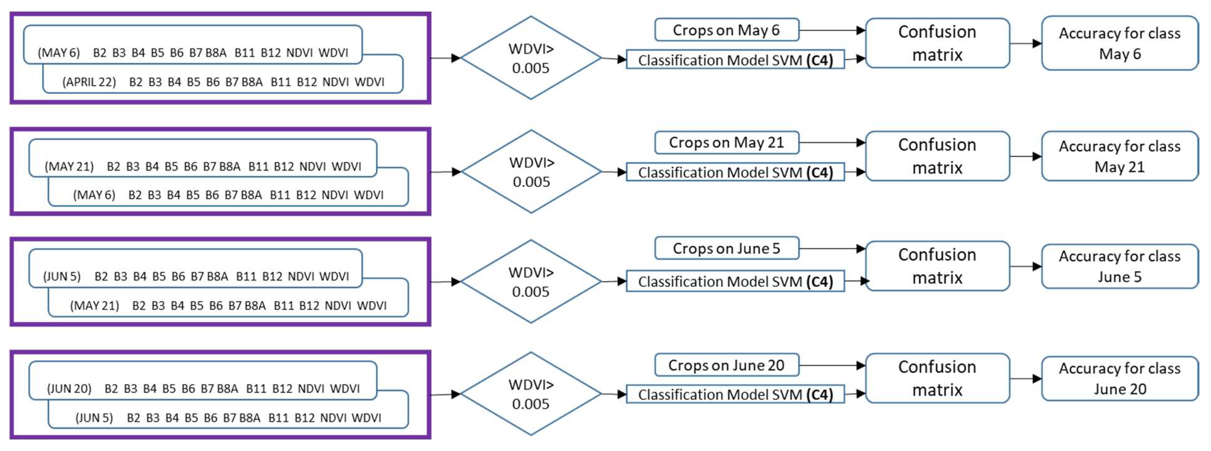
- Testing of the models in the next agricultural cycle
3. Results and Discussion
3.1. Results Obtained with the SVM Algorithm
3.2. Results Obtained with the BT Algorithm
3.3. Comparison of the Results Obtained with the Two Algorithms: SVM and BT
3.4. Test of the SVM Model in the Subsequent Cycle
4. Conclusions
Author Contributions
Funding
Institutional Review Board Statement
Informed Consent Statement
Data Availability Statement
Acknowledgments
Conflicts of Interest
References
- Orynbaikyzy, A.; Gessner, U.; Conrad, C. Crop type classification using a combination of optical and radar remote sensing data: A review. Int. J. Remote Sens. 2019, 40, 6553–6595. [Google Scholar] [CrossRef]
- Salehi, B.; Daneshfar, B.; Davidson, A.M. Accurate crop-type classification using multi-temporal optical and multi-polarization SAR data in an object-based image analysis framework. Int. J. Remote Sens. 2017, 38, 4130–4155. [Google Scholar] [CrossRef]
- Wójtowicz, M.; Wójtowicz, A.; Piekarczyk, J. Application of remote sensing methods in agriculture. Commun. Biometry Crop Sci. 2016, 11, 31–50. [Google Scholar]
- Peña-Barragán, J.M.; Ngugi, M.K.; Plant, R.E.; Six, J. Object-based crop identification using multiple vegetation indices, textural features and crop phenology. Remote Sens. Environ. 2011, 115, 1301–1316. [Google Scholar] [CrossRef]
- Canisius, F.; Shang, J.; Liu, J.; Huang, X.; Ma, B.; Jiao, X.; Geng, X.; Kovacs, J.M.; Walters, D. Tracking crop phenological development using multi-temporal polarimetric Radarsat-2 data. Remote Sens. Environ. 2018, 210, 508–518. [Google Scholar] [CrossRef]
- Delavarpour, N.; Koparan, C.; Nowatzki, J.; Bajwa, S.; Sun, X. A technical study on UAV characteristics for precision agriculture applications and associated practical challenges. Remote Sens. 2021, 13, 1204. [Google Scholar] [CrossRef]
- Pal, M.; Mather, P.M. Support vector machines for classification in remote sensing. Int. J. Remote Sens. 2005, 26, 1007–1011. [Google Scholar] [CrossRef]
- Amat Rodrigo, J. Máquinas de Vector Soporte (Support Vector Machines, SVMs). 2020. Available online: https://www.cienciadedatos.net/documentos/34_maquinas_de_vector_soporte_support_vector_machines#Bibliografía (accessed on 26 October 2021).
- Mathur, A.; Foody, G.M. Multiclass and Binary SVM Classification: Implications for Training and Classification Users. IEEE Geosci. Remote Sens. Lett. 2008, 5, 241–245. [Google Scholar] [CrossRef]
- Breiman, L. Bagging predictors. Mach. Learn. 1996, 24, 123–140. [Google Scholar] [CrossRef]
- Sutton, C.D. Classification and Regression Trees, Bagging, and Boosting; Elsevier Masson SAS: Paris, France, 2005. [Google Scholar]
- Tucker, C.J. Red and photographic infrared linear combinations for monitoring vegetation. Remote Sens. Environ. 1979, 8, 127–150. [Google Scholar] [CrossRef]
- Clevers, J.G.P.W. Application of the WDVI in estimating LAI at the generative stage of barley. ISPRS J. Photogramm. Remote Sens. 1991, 46, 37–47. [Google Scholar] [CrossRef]
- Yang, C.; Everitt, J.H.; Murden, D. Evaluating high resolution SPOT 5 satellite imagery for crop identification. Comput. Electron. Agric. 2011, 75, 347–354. [Google Scholar] [CrossRef]
- Saini, R.; Ghosh, S.K. Crop classification on single date Sentinel-2 imagery using random forest and support vector machine. Int. Arch. Photogramm. Remote Sens. Spat. Inf. Sci. 2018, 42, 683–688. [Google Scholar] [CrossRef]
- Martínez-Casasnovas, J.A.; Martín-Montero, A.; Auxiliadora Casterad, M. Mapping multi-year cropping patterns in small irrigation districts from time-series analysis of Landsat TM images. Eur. J. Agron. 2005, 23, 159–169. [Google Scholar] [CrossRef]
- Zheng, B.; Myint, S.W.; Thenkabail, P.S.; Aggarwal, R.M. A support vector machine to identify irrigated crop types using time-series Landsat NDVI data. Int. J. Appl. Earth Obs. Geoinf. 2015, 34, 103–112. [Google Scholar] [CrossRef]
- Defourny, P.; Bontemps, S.; Bellemans, N.; Cara, C.; Dedieu, G.; Guzzonato, E.; Hagolle, O.; Inglada, J.; Nicola, L.; Rabaute, T.; et al. Near real-time agriculture monitoring at national scale at parcel resolution: Performance assessment of the Sen2-Agri automated system in various cropping systems around the world. Remote Sens. Environ. 2019, 221, 551–568. [Google Scholar] [CrossRef]
- Lin, C.; Zhong, L.; Song, X.-P.; Dong, J.; Lobell, D.B.; Jin, Z. Early- and in-season crop type mapping without current-year ground truth: Generating labels from historical information via a topology-based approach. Remote Sens. Environ. 2022, 274, 22. [Google Scholar] [CrossRef]
- Cai, Y.; Guan, K.; Peng, J.; Wang, S.; Seifert, C.; Wardlow, B.; Li, Z. A high-performance and in-season classification system of field-level crop types using time-series Landsat data and a machine learning approach. Remote Sens. Environ. 2018, 10, 34–57. [Google Scholar] [CrossRef]
- Conrad, C.; Fritsch, S.; Zeidler, J.; Rücker, G.; Dech, S. Per-Field Irrigated Crop Classification in Arid Central Asia Using SPOT and ASTER Data. Remote Sens. 2010, 2, 1035–1056. [Google Scholar] [CrossRef]
- Hegarty-Craver, M.; Polly, J.; O’Neil, M.; Ujeneza, N.; Rineer, J.; Beach, R.H.; Lapidus, D.; Temple, D.S. Remote Crop Mapping at Scale: Using Satellite Imagery and UAV-Acquired Data as Ground Truth. Remote Sens. 2020, 12, 15. [Google Scholar] [CrossRef]
- Prins, A.J.; Van Niekerk, A. Crop type mapping using LiDAR, Sentinel-2 and aerial imagery with machine learning algorithms. Geo Spat. Inf. Sci. 2020, 24, 215–227. [Google Scholar] [CrossRef]
- Konduri, V.S.; Kumar, J.; Hargrove, W.W.; Hoffman, F.M.; Ganguly, A.R. Mapping crops within the growing season across the United States. Remote Sens. Environ. 2020, 251, 112048. [Google Scholar] [CrossRef]
- Tran, K.H.; Zhang, H.K.; McMaine, J.T.; Zhang, X.; Luo, D. 10 m crop type mapping using Sentinel-2 reflectance and 30 m cropland data layer product. Int. J. Appl. Earth Obs. Geoinf. 2022, 107, 102692. [Google Scholar] [CrossRef]
- Blickensdörfer, L.; Schwieder, M.; Pflugmacher, D.; Nendel, C.; Erasmi, S.; Hostert, P. Mapping of crop types and crop sequences with combined time series of Sentinel-1, Sentinel-2 and Landsat 8 data for Germany. Remote Sens. Environ. 2022, 269, 19. [Google Scholar] [CrossRef]
- Congalton, R.G.; Green, K. Sample design considerations. In Assessing the Accuracy of Remotely Sensed Data: Principles and Practices; CRC Press: Boca Raton, FL, USA, 2009; pp. 63–83. [Google Scholar]
- McCoy, R.M. Field Methods in Remote Sensing; The Guilford Press: New York, NY, USA, 2005; ISBN 9781593850791. [Google Scholar]
- Guan, X.; Huang, C.; Liu, G.; Meng, X.; Liu, Q. Mapping rice cropping systems in Vietnam using an NDVI-based time-series similarity measurement based on DTW distance. Remote Sens. 2016, 8, 19. [Google Scholar] [CrossRef]
- Pan, Z.; Huang, J.; Zhou, Q.; Wang, L.; Cheng, Y.; Zhang, H.; Blackburn, G.A.; Yan, J.; Liu, J. Mapping crop phenology using NDVI time-series derived from HJ-1 A/B data. Int. J. Appl. Earth Obs. Geoinf. 2015, 34, 188–197. [Google Scholar] [CrossRef]
- Leite, P.B.C.; Feitosa, R.Q.; Formaggio, A.R.; Da Costa, G.A.O.P.; Pakzad, K.; Sanches, I.D.A. Hidden Markov Models for crop recognition in remote sensing image sequences. Pattern Recognit. Lett. 2011, 32, 19–26. [Google Scholar] [CrossRef]
- Siachalou, S.; Mallinis, G.; Tsakiri-Strati, M. Analysis of Time-Series Spectral Index Data to Enhance Crop Identification over a Mediterranean Rural Landscape. IEEE Geosci. Remote Sens. Lett. 2017, 14, 1508–1512. [Google Scholar] [CrossRef]
- Alagic, Z.; Diaz Cardenas, J.; Halldorsson, K.; Grozman, V.; Wallgren, S.; Suzuki, C.; Helmenkamp, J.; Koskinen, S.K. Deep learning versus iterative image reconstruction algorithm for head CT in trauma. Emerg. Radiol. 2022, 29, 339–352. [Google Scholar] [CrossRef]
- Altman, D.G. Practical Statistics for Medical Research; CRC Press: Boca Raton, FL, USA, 1990; ISBN 9781000228816. [Google Scholar]
- Kussul, N.; Lemoine, G.; Gallego, F.J.; Skakun, S.V.; Lavreniuk, M.; Shelestov, A.Y. Parcel-Based Crop Classification in Ukraine Using Landsat-8 Data and Sentinel-1A Data. IEEE J. Sel. Top. Appl. Earth Obs. Remote Sens. 2016, 9, 2500–2508. [Google Scholar] [CrossRef]
- de Souza, C.H.W.; Mercante, E.; Johann, J.A.; Camargo Lamparelli, R.A.; Uribe-opazo, A. Mapping and discrimination of soya bean and corn crops using spectro- temporal profiles of vegetation indices. Int. J. Remote Sens. 2015, 36, 1809–1824. [Google Scholar] [CrossRef]
- Rahman, S.A.Z.; Mitra, K.C.; Islam, S.M.M. Soil Classification using Machine Learning Methods and Crop Suggestion Based on Soil Series. In Proceedings of the 2018 21st International Conference of Computer and Information Technology (ICCIT), Dhaka, Bangladesh, 21–23 December 2018. [Google Scholar]
- Chakhar, A.; Hernández-López, D.; Ballesteros, R.; Moreno, M.A. Improving the Accuracy of Multiple Algorithms for Crop Classification by Integrating Sentinel-1 Observations with Sentinel-2 Data. Remote Sens. 2021, 13, 243. [Google Scholar] [CrossRef]
- Adam, E.; Mutanga, O.; Odindi, J.; Abdel-Rahman, E.M. Land-use/cover classification in a heterogeneous coastal landscape using RapidEye imagery: Evaluating the performance of random forest and support vector machines classifiers. Int. J. Remote Sens. 2014, 35, 3440–3458. [Google Scholar] [CrossRef]
- Löw, F.; Schorcht, G.; Michel, U.; Dech, S.; Conrad, C. Per-field crop classification in irrigated agricultural regions in middle Asia using random forest and support vector machine ensemble. In Proceedings of the Earth Resources and Environmental Remote Sensing/GIS Applications III, Edinburgh, UK, 24–26 September 2012; Volume 8538, pp. 187–197. [Google Scholar]
- Mardani, M.; Mardani, H.; Simone, L.D.; Varas, S.; Kita, N.; Saito, T. Integration of Machine Learning and Open Access Geospatial Data for Land Cover Mapping. Remote Sens. 2019, 11, 1907. [Google Scholar] [CrossRef]
- Pal, M. Random forest classifier for remote sensing classification. Int. J. Remote Sens. 2005, 26, 217–222. [Google Scholar] [CrossRef]
- Macedo-Cruz, A.; Pajares, G.; Santos, M.; Villegas-Romero, I. Digital Image Sensor-Based Assessment of the Status of Oat (Avena sativa L.) Crops after Frost Damage. Sensors 2011, 11, 6015–6036. [Google Scholar] [CrossRef]
- Cohen, J. A coefficient of agreement for nominal scales. Educ. Psychol. Meas. 1960, 20, 37–46. [Google Scholar] [CrossRef]


| Author | Range of Images | Images | Training Samples | Classification Method | Within-Season Mapping |
|---|---|---|---|---|---|
| Martínez et al. [16] | multi-year | Landsat TM y ETM | Fields survey | Cross classification (IDRISI sotware) | No |
| Zheng et al. [17] | Agricultural year | Landsat TM y ETM | Fields survey | SVM | No |
| Conrad et al. [21] | Crop Cycle | SPOT 5 y ASTER | Expert knowledge | Rules of classification | No |
| Saini and Ghosh [15] | Crop Cycle | Sentinel 2 | Fields Survey | RF and SVM | No |
| Yang et al. [14] | Crop Cycle | SPOT 5 | Fields survey | MD, M-distance, MLE, SAM and SVM | No |
| Hegarty-Craver et al. [22] | Crop Cycle | Image UAV, Sentinel 1 y Sentinel 2 | Fields survey | RF | No |
| Prins and Van Niekerk [23] | Crop Cycle | Aerial Image, LIDAR image, Sentinel 2 | Crop type database | RF, DTs, XGBoost, k-NN, LR, NB, NN, d-NN, SVM-L, and SVM RBF | No |
| Cai et al. [20] | Multi-year | Landsat TM y ETM | CDL (USDA) | d-NN | Yes |
| Konduri et al. [24] | Multi-year | MODIS | CDL (USDA) | unsupervised classification (phenoregions) | Yes |
| Lin et al. [19] | Multi-year | Sentinel 2, Landsat 8 | CDL (USDA) | RF | Yes |
| Tran et al. [25] | Crop Cycle | Sentinel 2 | CDL (USDA) | RF | No |
| Blickensdörfer et al. [26] | Multi-year | Sentinel 1 Sentinel 2 Landsat 8 | Land Parcel Information System (LPIS). | RF | No |
| Defourny et al. [18] | Multi-year | Sentinel 2 | Ground truth data | RF | Yes |
| Crop | March | April | May | June | July | August | September | October | ||||||||||||||||||||||||
|---|---|---|---|---|---|---|---|---|---|---|---|---|---|---|---|---|---|---|---|---|---|---|---|---|---|---|---|---|---|---|---|---|
| Bean | ||||||||||||||||||||||||||||||||
| Corn | ||||||||||||||||||||||||||||||||
| Alfalfa | ||||||||||||||||||||||||||||||||
| Month | Available Images | Images Used | Image Acquisition Date | ||||||
|---|---|---|---|---|---|---|---|---|---|
| April | 6 | 6 | 2 | 7 | 12 | 17 | 22 | 27 | |
| May | 6 | 6 | 2 | 7 | 12 | 17 | 22 | 27 | |
| June | 6 | 4 | 1 | 6 | 11 | 16 | 21 | 26 | |
| July | 7 | 4 | 1 | 6 | 11 | 16 | 21 | 26 | 31 |
| August | 6 | 6 | 5 | 10 | 15 | 20 | 25 | 30 | |
| September | 6 | 1 | 4 | ||||||
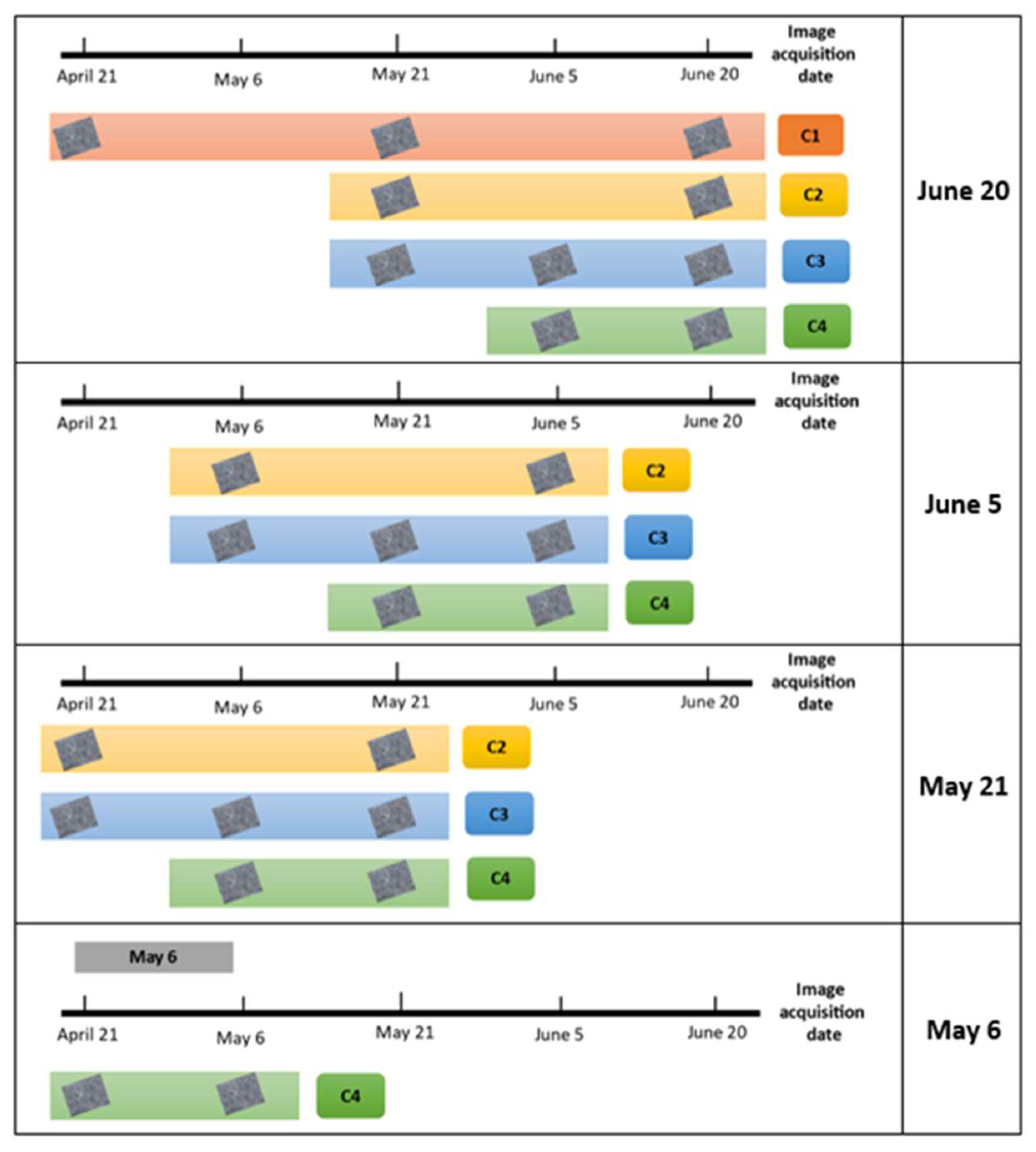
| Combination | Number of Descriptors | Number of Images | Dates of Scenes Used | ||
|---|---|---|---|---|---|
| C1 | 33 | 3 | CD | 30 DB (6 PS) | 60 DB (12 PS) |
| C2 | 22 | 2 | CD | 30 DB (6 PS) | |
| C3 | 33 | 3 | CD | 15 DB (3 PS) | 30 DB (6 PS) |
| C4 | 22 | 2 | CD | 15 DB (3 PS) | |
| Combination | Scenes Used | ||
|---|---|---|---|
| C1 | 6 July 2019 | 6 June 2019 | 7 May 2019 |
| C2 | 6 July 2019 | 6 June 2019 | |
| C3 | 6 July 2019 | 21 June 2019 | 6 June 2019 |
| C4 | 6 July 2019 | 21 June 2019 | |
| Cultivation Type | Date of Analysis | Dates of Images or Scenes Included in the Database | ||
|---|---|---|---|---|
| corn 1 | 6 September | 4 September | 5 August | 6 July |
| corn 1 | 5 August | 5 August | 6 July | 6 June |
| corn 1 | 6 July | 6 July | 6 June | 7 May |
| corn 1 | 6 June | 6 June | 7 May | 7 April |
| corn 77 | 4 September | 4 September | 5 August | 6 July |
| corn 77 | 5 August | 5 August | 6 July | 6 June |
| corn 77 | 6 July | 6 July | 6 June | 7 May |
| corn 77 | 6 June | 6 June | 7 May | 7 April |
| Combination | Kappa Coefficient | Overall Accuracy % | Corn | Alfalfa | Bean | |||
|---|---|---|---|---|---|---|---|---|
| PA % | UA % | PA % | UA % | PA % | UA % | |||
| C1 | 0.91 | 94.8 | 97.2 | 96.0 | 94.1 | 97.4 | 89.2 | 87.5 |
| C2 | 0.89 | 93.4 | 95.8 | 95.1 | 94.6 | 96.0 | 85.2 | 84.9 |
| C3 | 0.91 | 94.4 | 96.6 | 95.0 | 93.9 | 98.0 | 89.0 | 87.5 |
| C4 | 0.86 | 91.5 | 94.3 | 93.3 | 90.5 | 97.4 | 85.1 | 80.4 |
| Combination | Kappa Coefficient | Overall Accuracy % | Corn | Alfalfa | Bean | |||
|---|---|---|---|---|---|---|---|---|
| PA % | UA % | PA % | UA % | PA % | UA % | |||
| C1 | 0.87 | 91.8 | 95.8 | 95.9 | 89.3 | 91.8 | 84.9 | 81.3 |
| C2 | 0.79 | 87.4 | 94.2 | 90.4 | 87.9 | 88.3 | 67.6 | 75.9 |
| C3 | 0.84 | 90.6 | 95.1 | 91.5 | 93.1 | 94.1 | 73.8 | 81.6 |
| C4 | 0.74 | 84.9 | 93.0 | 85.2 | 89.6 | 90.9 | 57.8 | 74.5 |
| 3 scenes | C3 | C1 | ||||
| SVM | BT | SVM | BT | |||
| Kappa coefficient | 0.91 | 0.84 | 0.91 | 0.87 | ||
| Global accuracy | 94.4% | 90.6% | 94.8% | 91.8% | ||
| 2 scenes | C4 | C2 | ||||
| SVM | BT | SVM | BT | |||
| 0.86 | 0.74 | 0.89 | 0.79 | Kappa coefficient | ||
| 91.5% | 84.9% | 93.4% | 87.4% | Overall accuracy | ||
| 15 days | 30 days | 60 days | ||||
| Combination | Kappa Coefficient | Overall Accuracy % | Corn | Alfalfa | Bean | |||
|---|---|---|---|---|---|---|---|---|
| PA % | UA % | PA % | UA % | PA % | UA % | |||
| C4 | 0.53 | 71.9 | 67.2 | 94.3 | 80.5 | 82.4 | 77.1 | 14.2 |
| Combination | Kappa Coefficient | Overall Accuracy % | Corn | Alfalfa | Bean | |||
|---|---|---|---|---|---|---|---|---|
| PA % | UA % | PA % | UA % | PA % | UA % | |||
| C2 | 0.68 | 83.1 | 81.7 | 95.5 | 89.3 | 76.2 | 57.1 | 30.8 |
| C3 | 0.65 | 81.0 | 78.5 | 95.3 | 85.5 | 80.6 | 80.0 | 25.2 |
| C4 | 0.63 | 80.0 | 77.7 | 95.0 | 83.3 | 80.3 | 82.5 | 24.3 |
| Combination | Kappa Coefficient | Overall Accuracy % | Corn | Alfalfa | Bean | |||
|---|---|---|---|---|---|---|---|---|
| PA % | UA % | PA % | UA % | PA % | UA % | |||
| C2 | 0.70 | 85.2 | 89.2 | 91.2 | 81.1 | 84.6 | 52.6 | 32.3 |
| C3 | 0.72 | 86.2 | 86.8 | 95.1 | 88.6 | 79.0 | 60.5 | 40.4 |
| C4 | 0.72 | 85.9 | 87.5 | 93.9 | 86.7 | 80.6 | 56.4 | 37.3 |
| Combination | Kappa Coefficient | Overall Accuracy % | Corn | Alfalfa | Bean | |||
|---|---|---|---|---|---|---|---|---|
| PA % | UA % | PA % | UA % | PA % | UA % | |||
| C1 | 0.70 | 84.4 | 82.6 | 95.5 | 90.5 | 79.5 | 62.1 | 28.6 |
| C2 | 0.74 | 87.5 | 89.4 | 94.0 | 88.2 | 83.5 | 51.4 | 36.7 |
| C3 | 0.73 | 86.8 | 86.9 | 94.9 | 89.7 | 80.0 | 61.8 | 41.2 |
| C4 | 0.73 | 86.9 | 88.2 | 94.0 | 87.5 | 83.4 | 58.8 | 35.1 |
Publisher’s Note: MDPI stays neutral with regard to jurisdictional claims in published maps and institutional affiliations. |
© 2022 by the authors. Licensee MDPI, Basel, Switzerland. This article is an open access article distributed under the terms and conditions of the Creative Commons Attribution (CC BY) license (https://creativecommons.org/licenses/by/4.0/).
Share and Cite
Espinosa-Herrera, J.M.; Macedo-Cruz, A.; Fernández-Reynoso, D.S.; Flores-Magdaleno, H.; Fernández-Ordoñez, Y.M.; Soria-Ruíz, J. Monitoring and Identification of Agricultural Crops through Multitemporal Analysis of Optical Images and Machine Learning Algorithms. Sensors 2022, 22, 6106. https://doi.org/10.3390/s22166106
Espinosa-Herrera JM, Macedo-Cruz A, Fernández-Reynoso DS, Flores-Magdaleno H, Fernández-Ordoñez YM, Soria-Ruíz J. Monitoring and Identification of Agricultural Crops through Multitemporal Analysis of Optical Images and Machine Learning Algorithms. Sensors. 2022; 22(16):6106. https://doi.org/10.3390/s22166106
Chicago/Turabian StyleEspinosa-Herrera, José M., Antonia Macedo-Cruz, Demetrio S. Fernández-Reynoso, Héctor Flores-Magdaleno, Yolanda M. Fernández-Ordoñez, and Jesús Soria-Ruíz. 2022. "Monitoring and Identification of Agricultural Crops through Multitemporal Analysis of Optical Images and Machine Learning Algorithms" Sensors 22, no. 16: 6106. https://doi.org/10.3390/s22166106