Indoor Path-Planning Algorithm for UAV-Based Contact Inspection

 , , and
Abstract
:1. Introduction
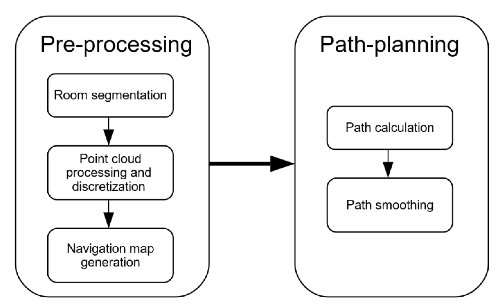
2. Methodology
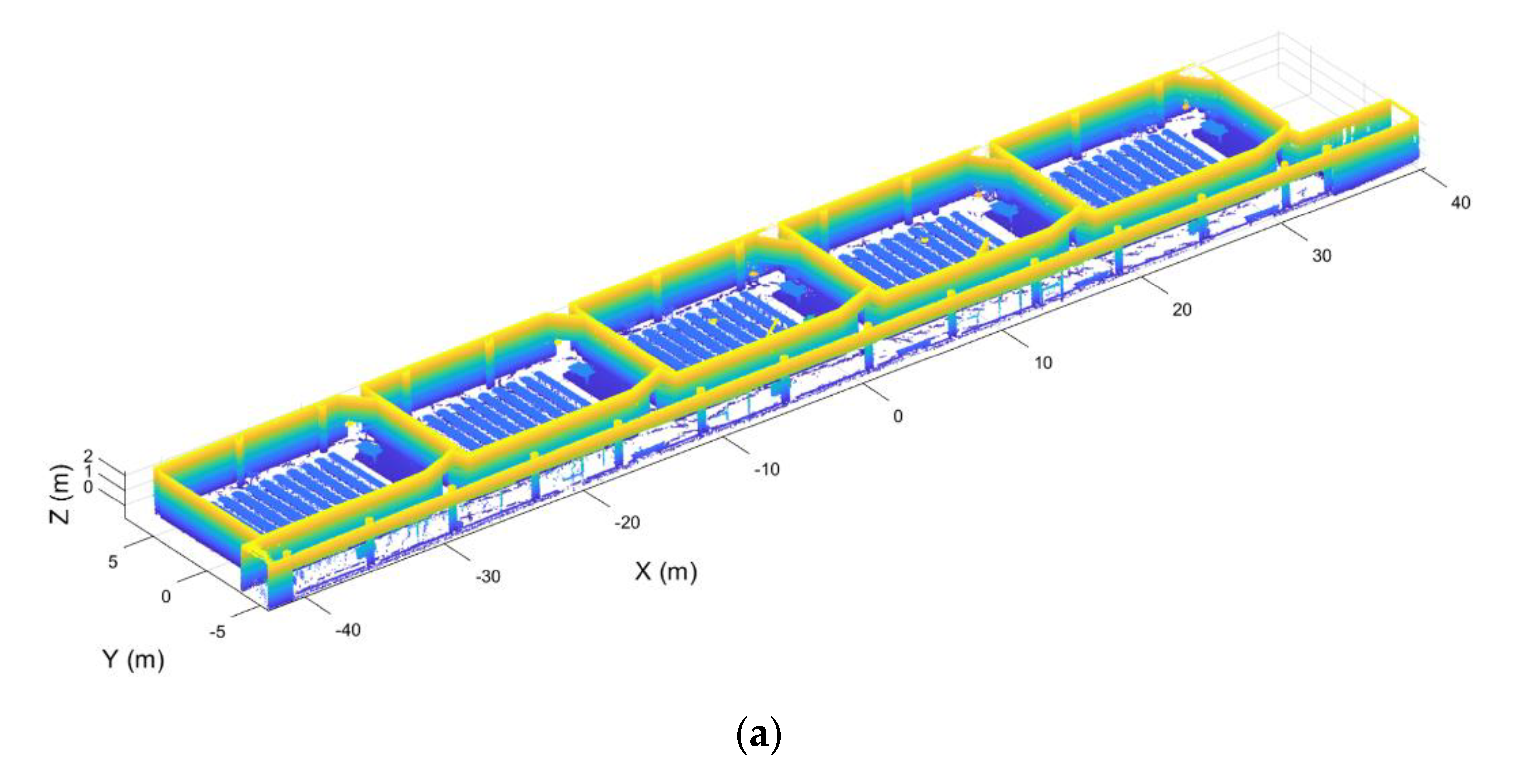
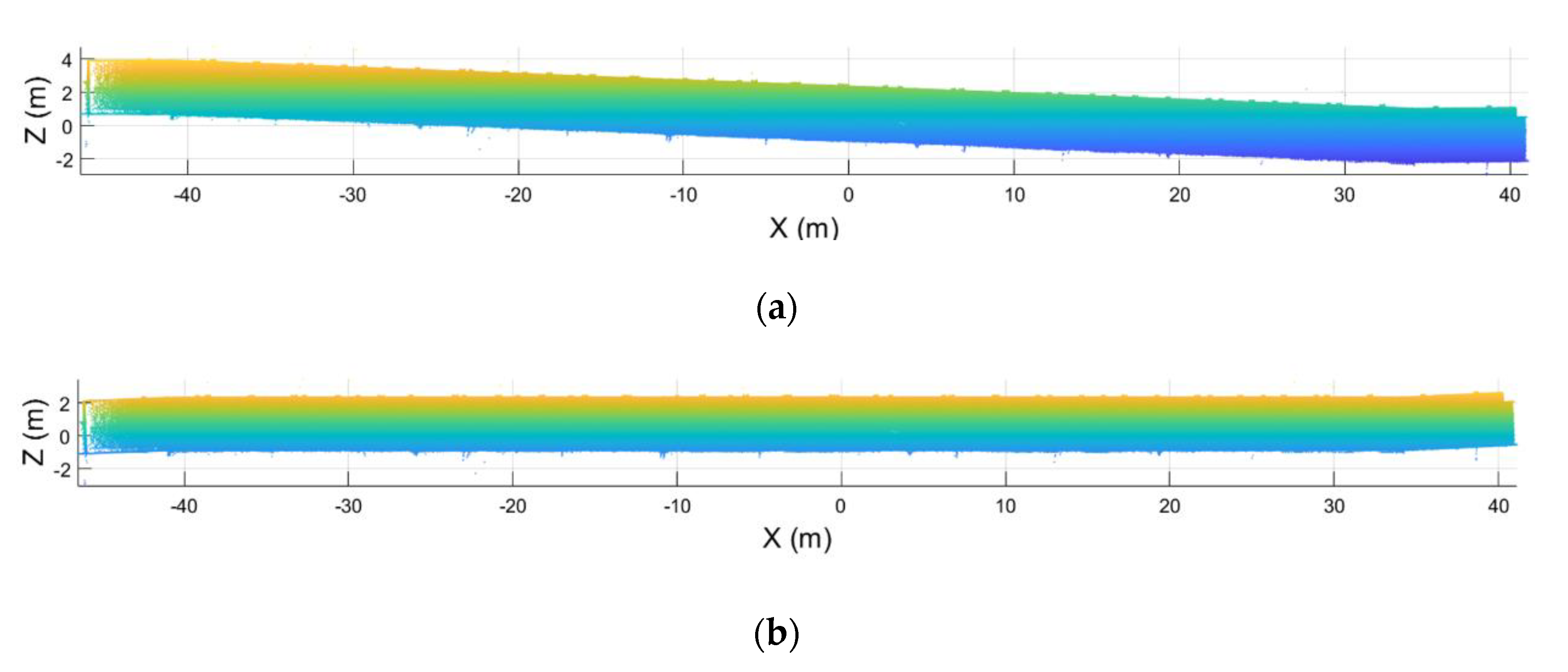
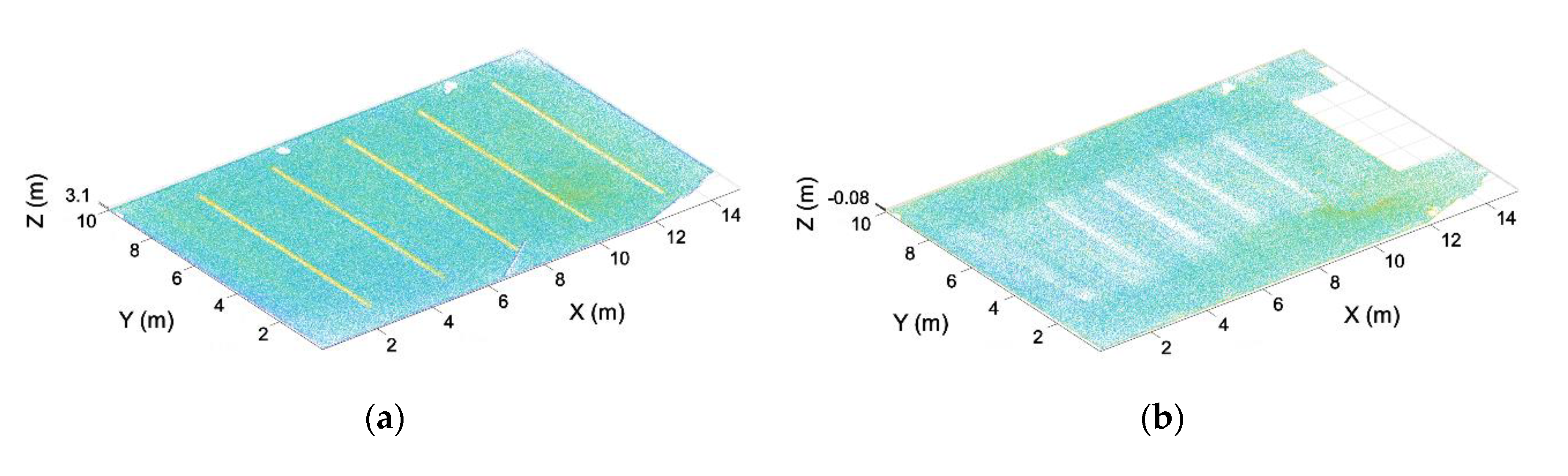
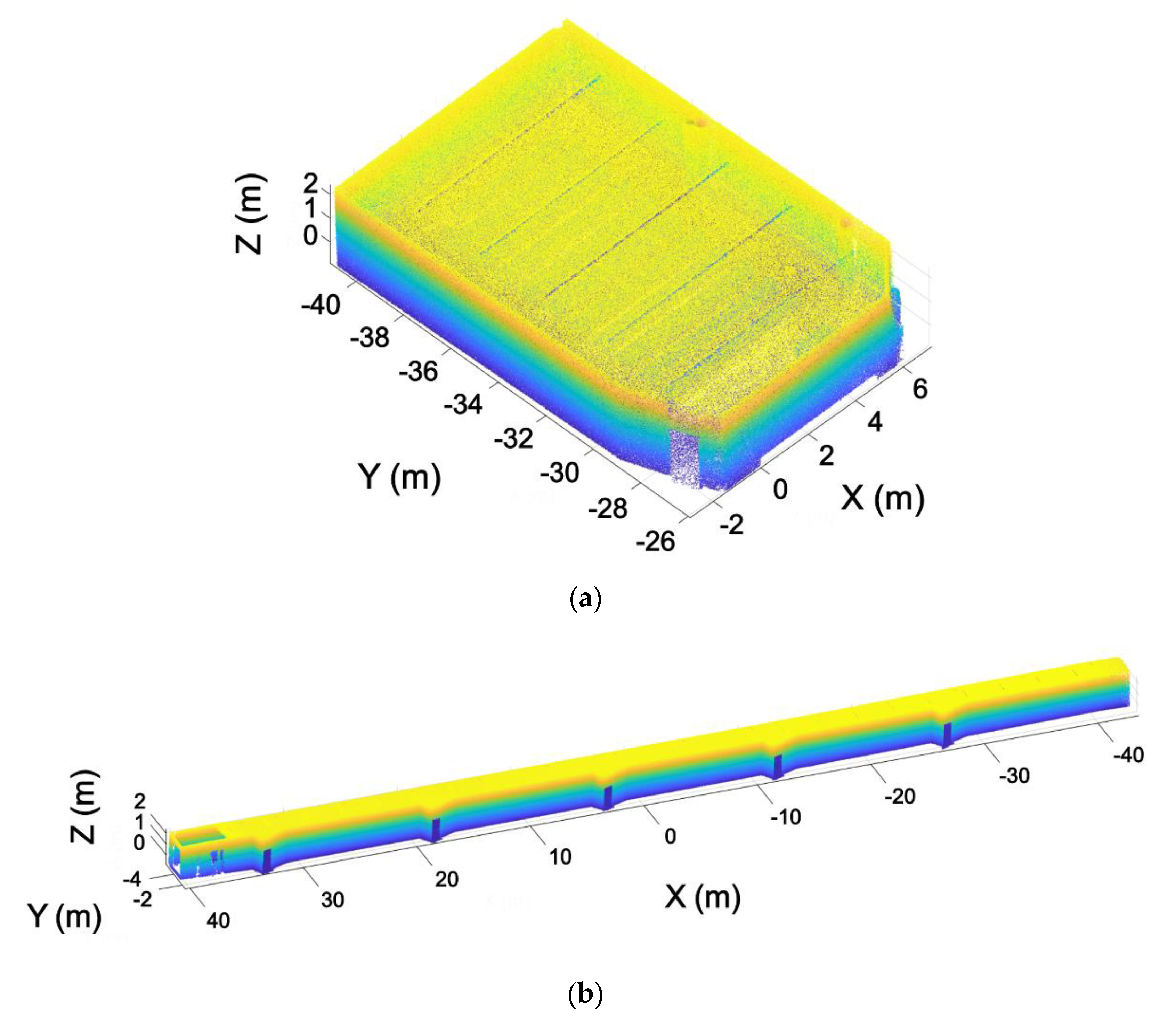
2.1. Point Cloud Pre-Processing
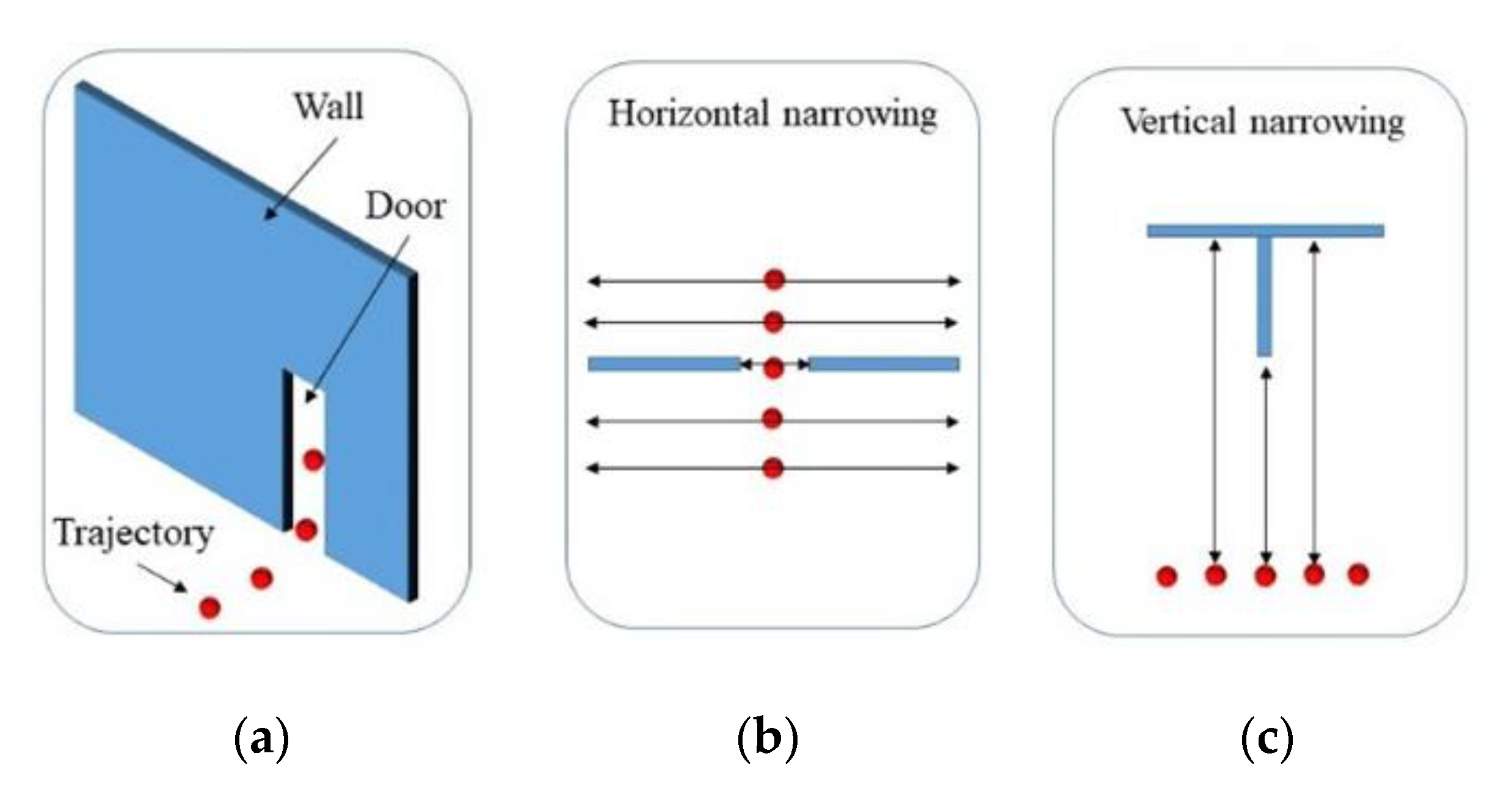
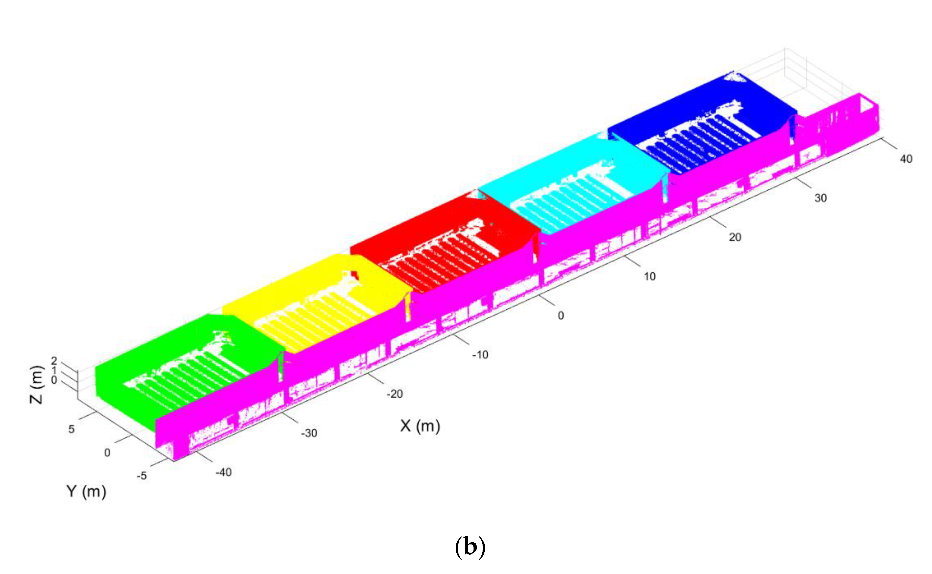
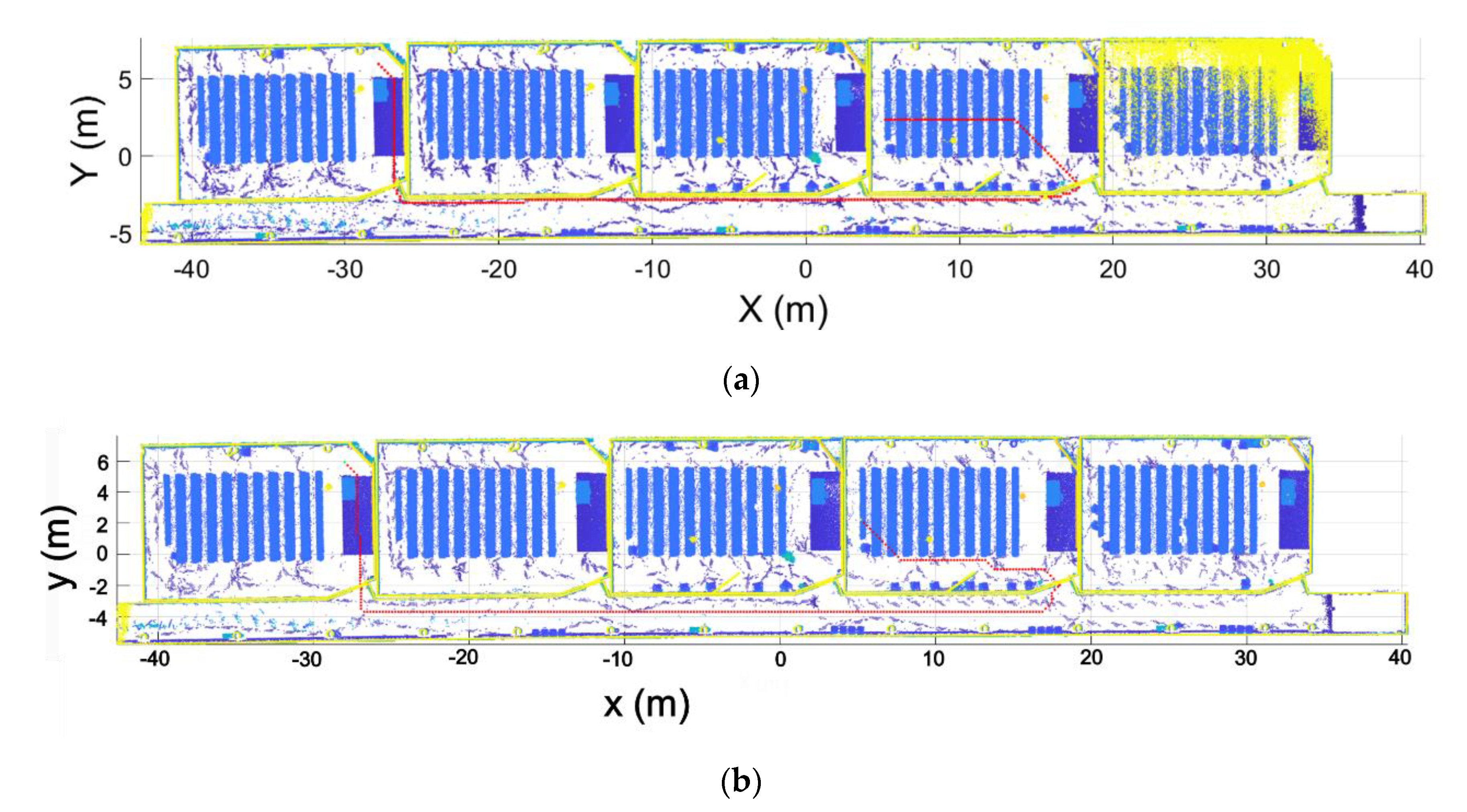
2.1.1. Room Segmentation
| Algorithm 1 Door Location Algorithm |
|
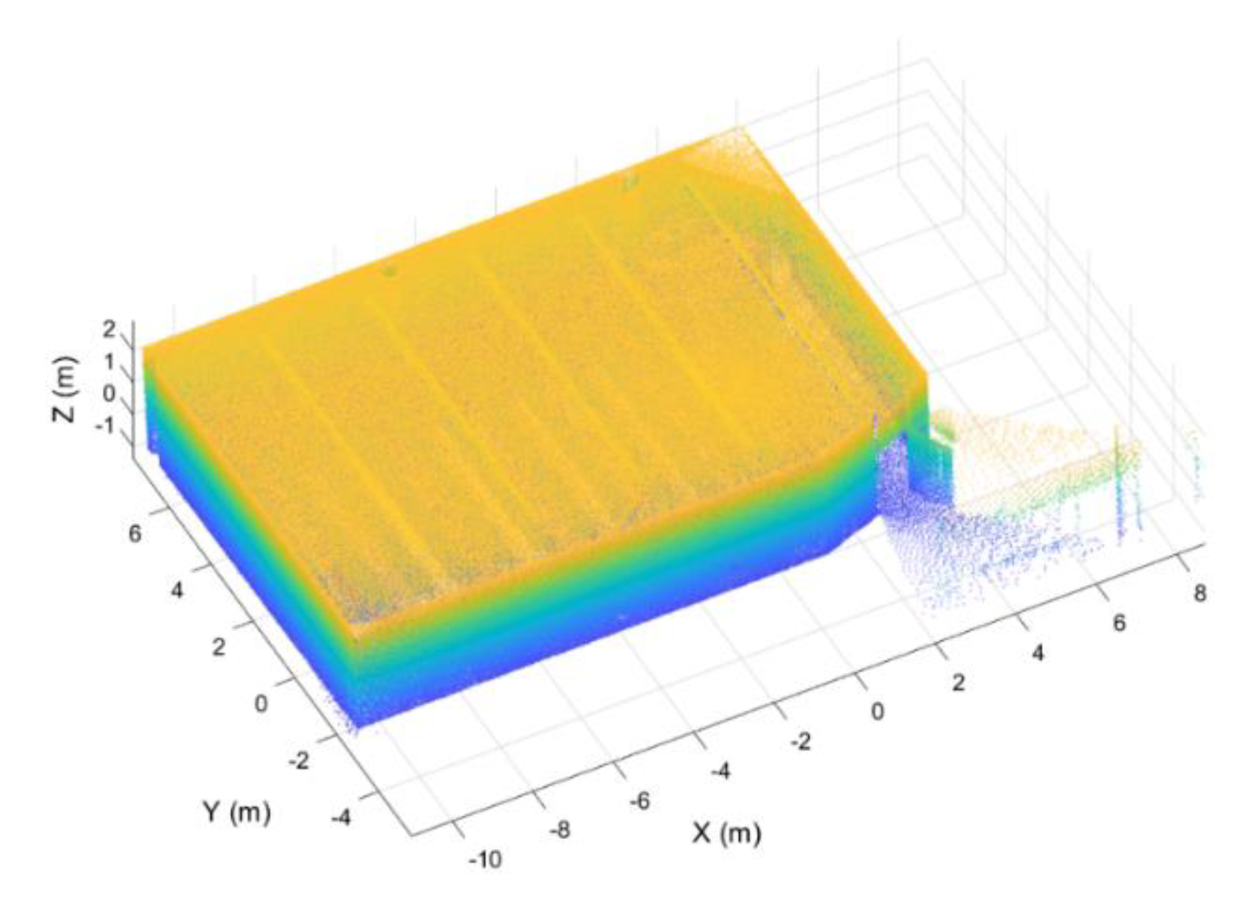
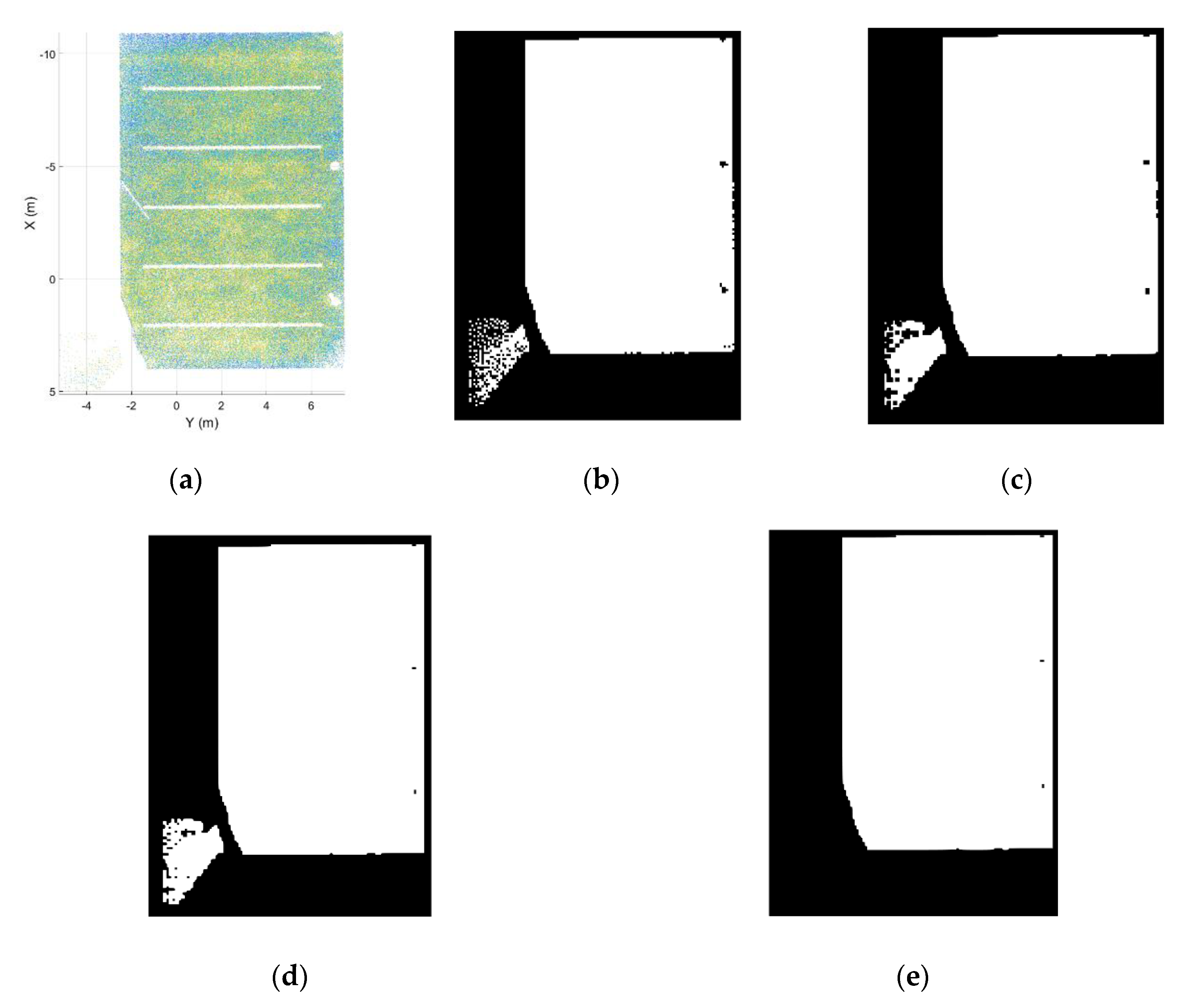
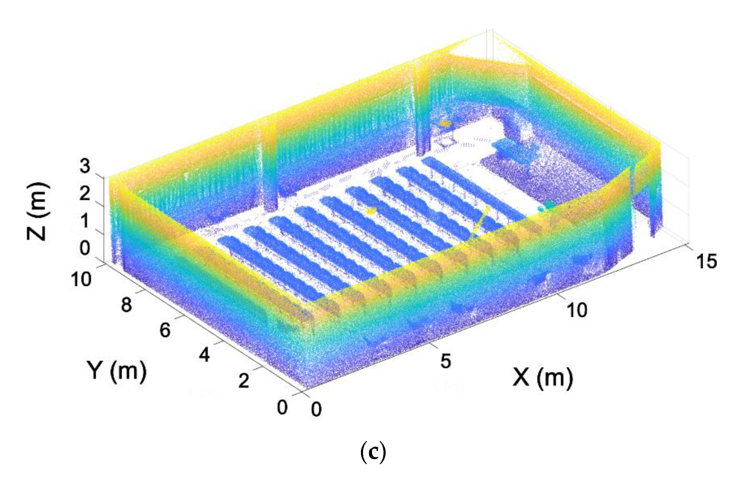
2.1.2. Point Cloud Pre-Processing
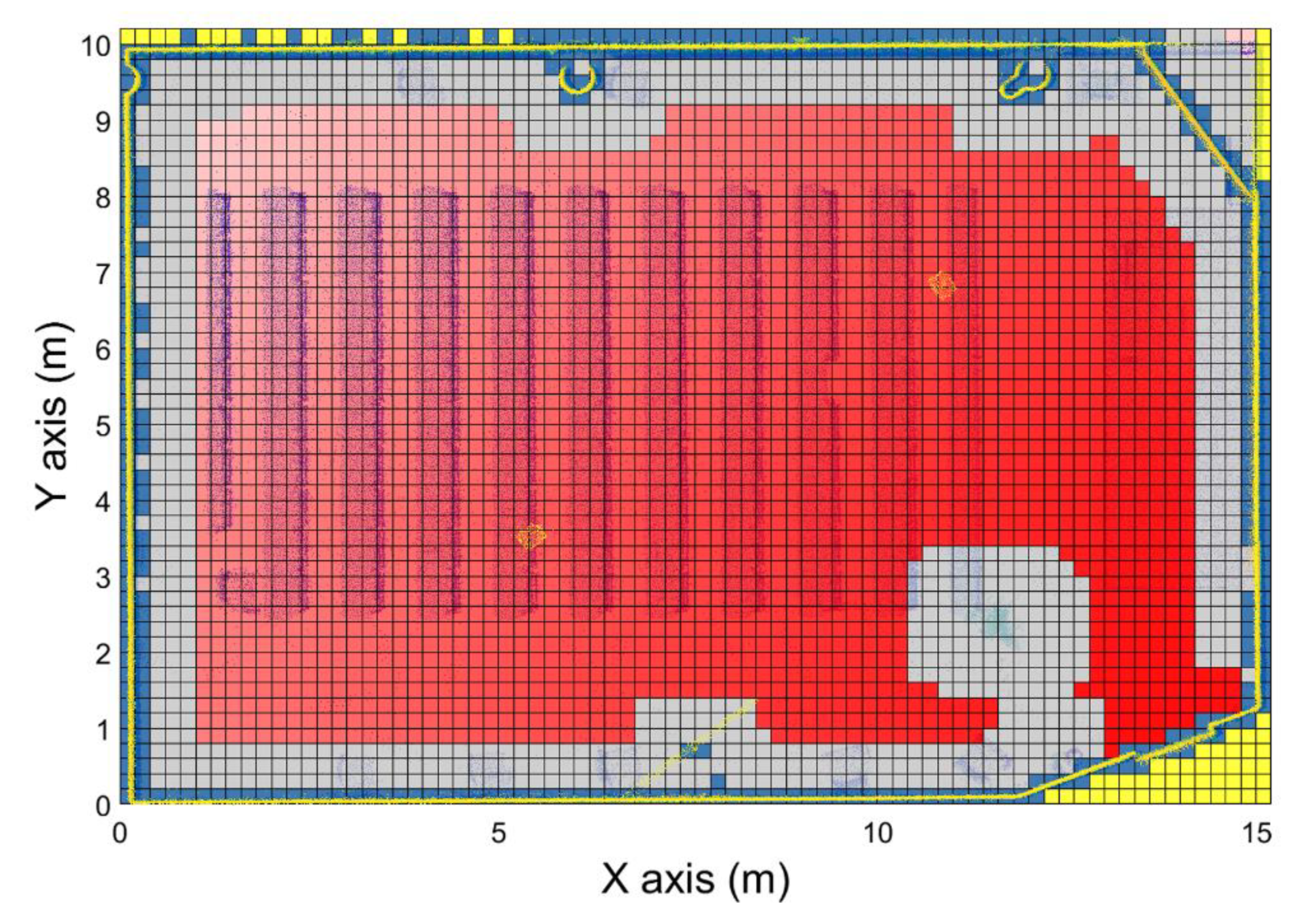
- Empty: Voxels that do not contain points inside.
- Occupied: Voxels that contain points inside.
- Security-offset: Empty voxels that are near an occupied one, and therefore, are not navigable by the drone.
- Exterior: Empty voxels that are outside the room.
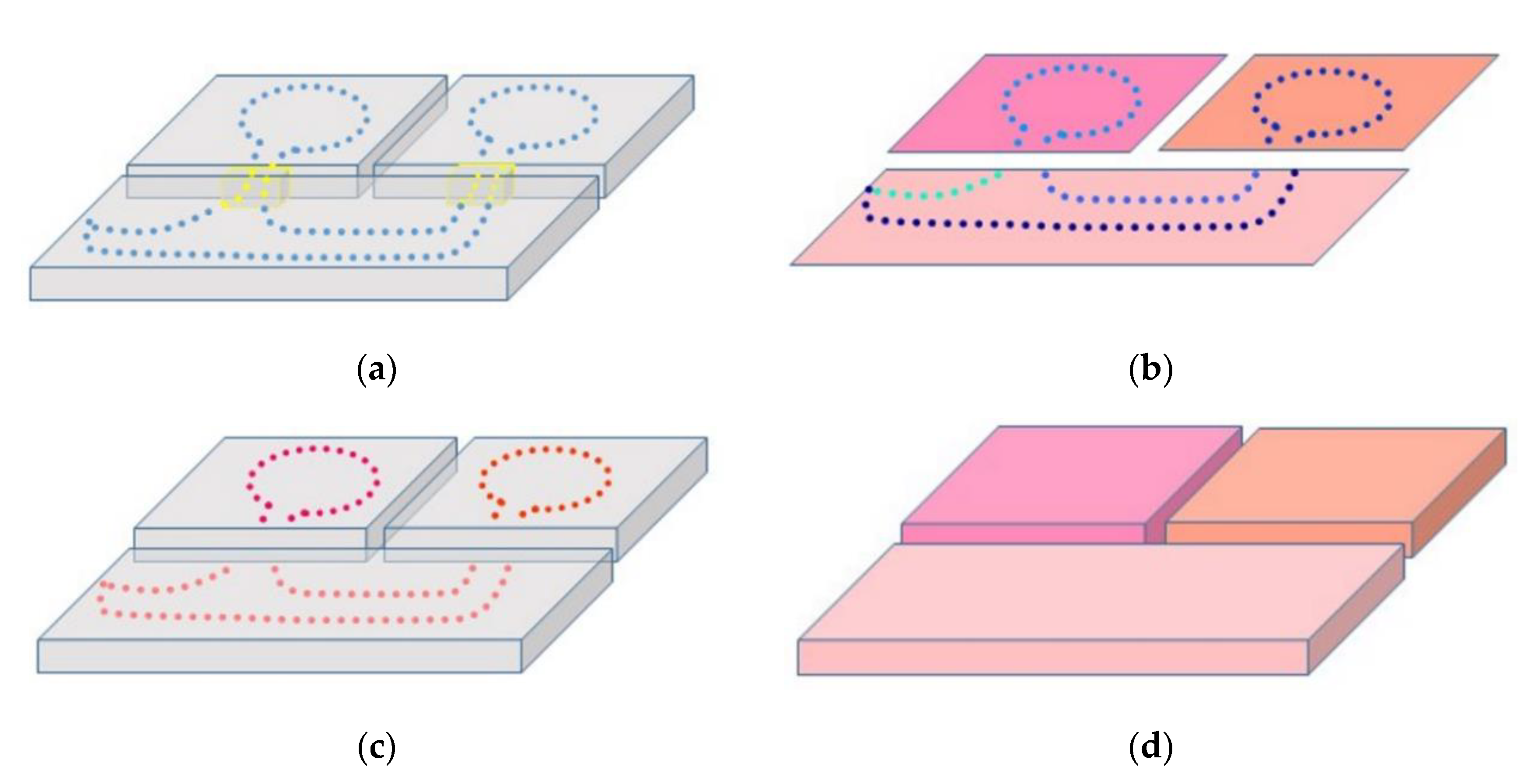
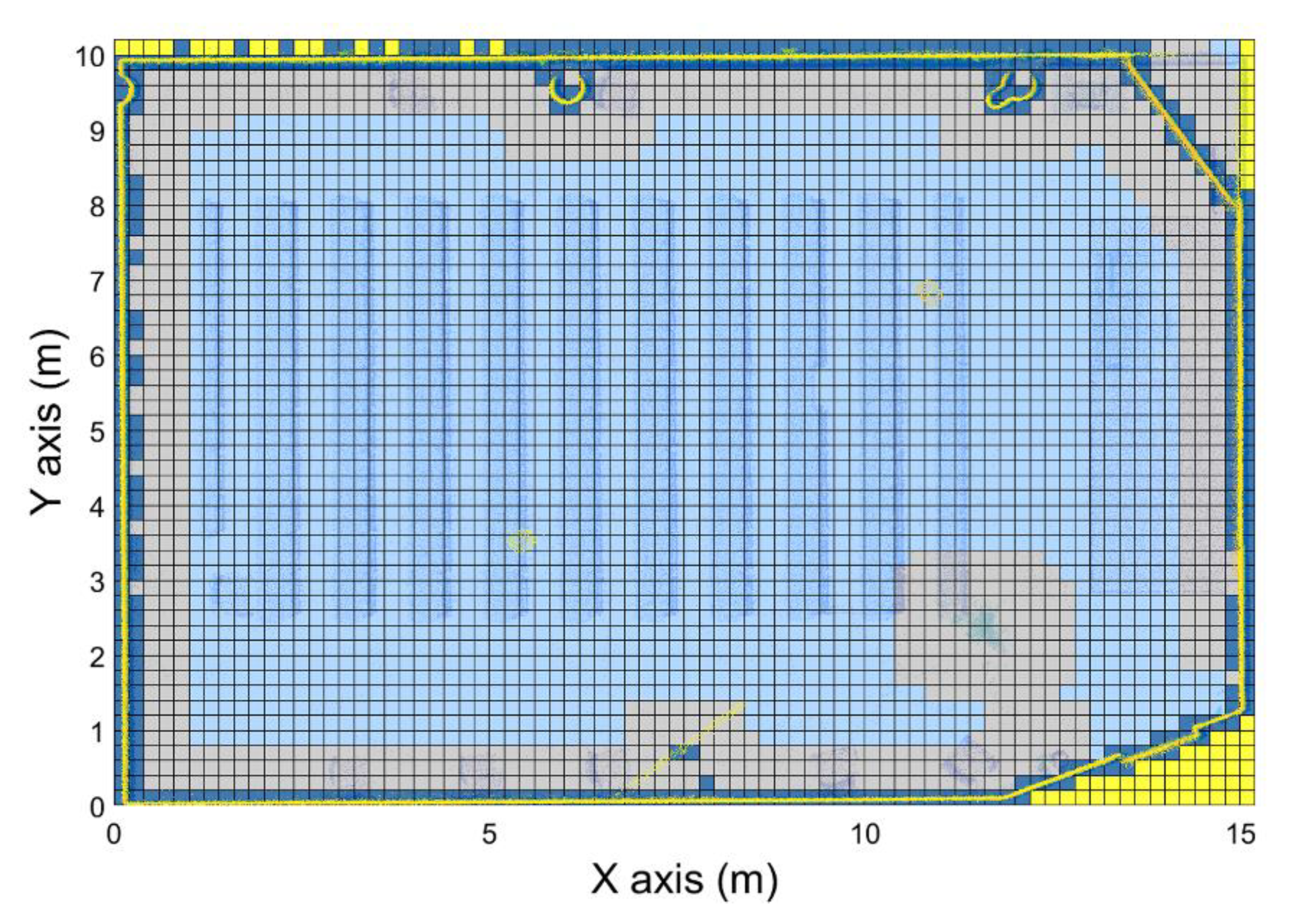
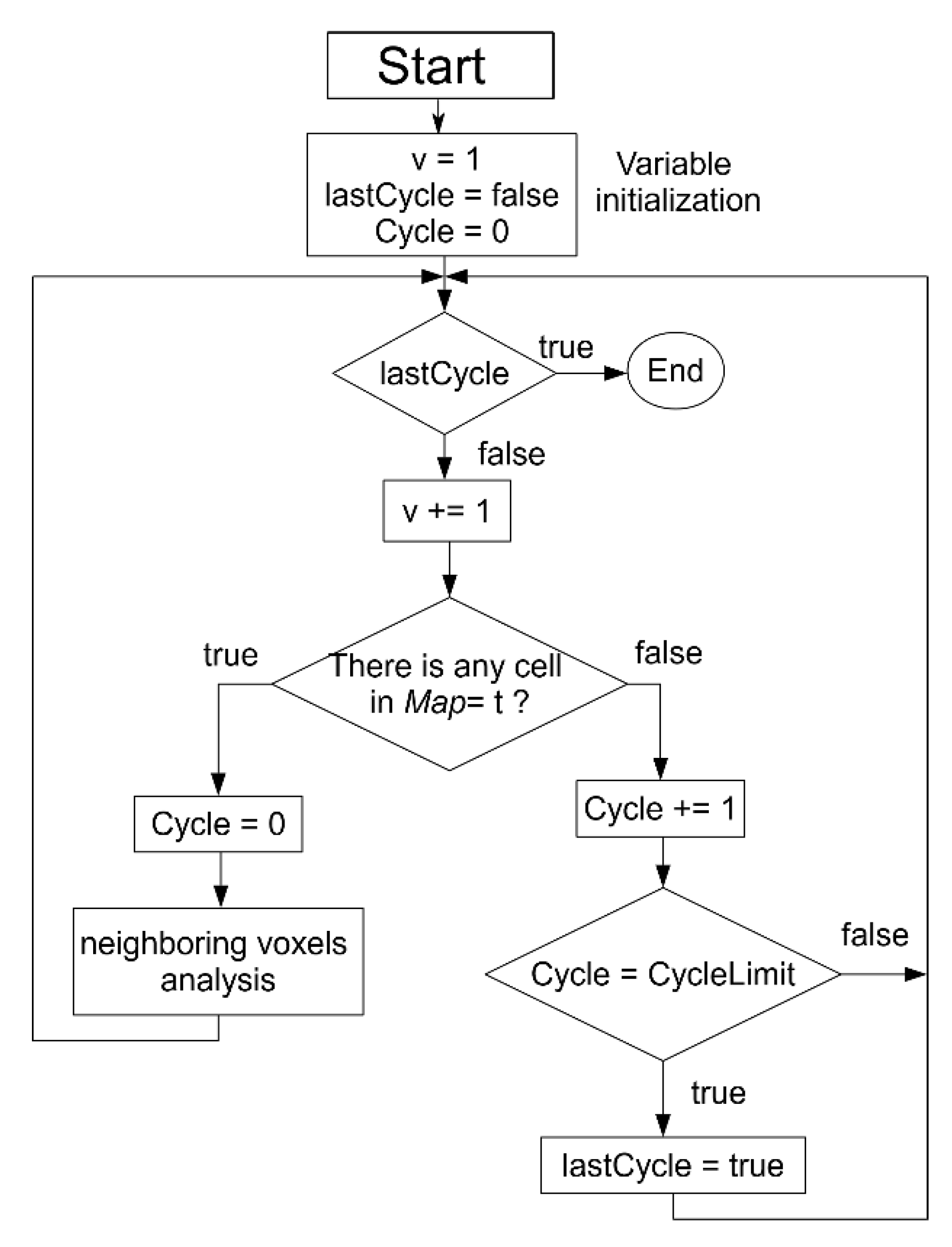
2.1.3. Navigation Map Generation
- Target voxel is the empty voxel that contains the door position and labeled with a “1”.
- Navigable voxels are empty voxels directly connected to the target voxel, meaning that there is at least one path from the voxel to the target. The label of these voxels depends on the number of surrounding voxels and the distance to the target.
- Nonnavigable voxels are empty voxels that are not directly connected to the target voxel, meaning that there is no possible path between them and the target voxel. These voxels are given a label value of “−1”.
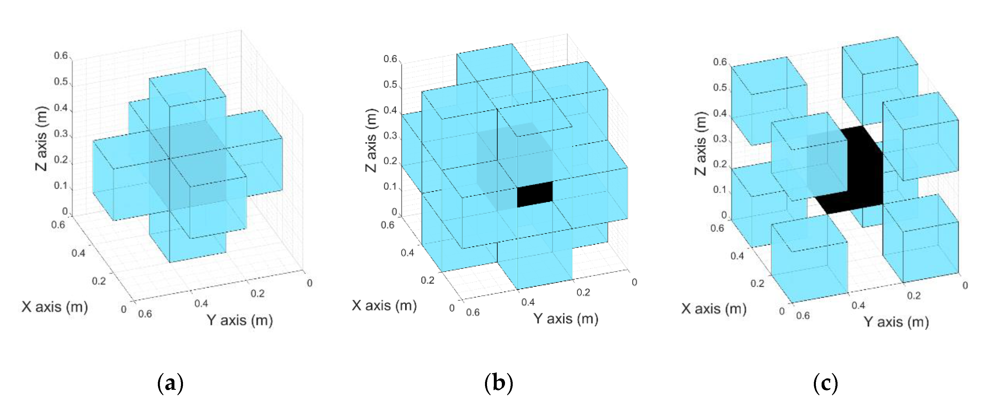
- Common face: Voxels surrounding the study voxels that have a common face. This means that the surrounding voxels and the study one have two coincident indices.
- Common edge: Voxels surrounding the study voxel that have a common edge. This means that the surrounding voxels and the study one have one coincident index.
- Common vertex: Voxels surrounding the study voxel that have a common vertex. This means that the surrounding voxels and the study voxel do not have any coincident indices.
- The route cannot pass through the same room twice.
- If two or more routes pass through the same room, the one containing the lower number of rooms is selected as the best route.
- If two routes are valid and do not share any part of the path, that containing the lowest number of waypoints, i.e., the shortest path, is selected.
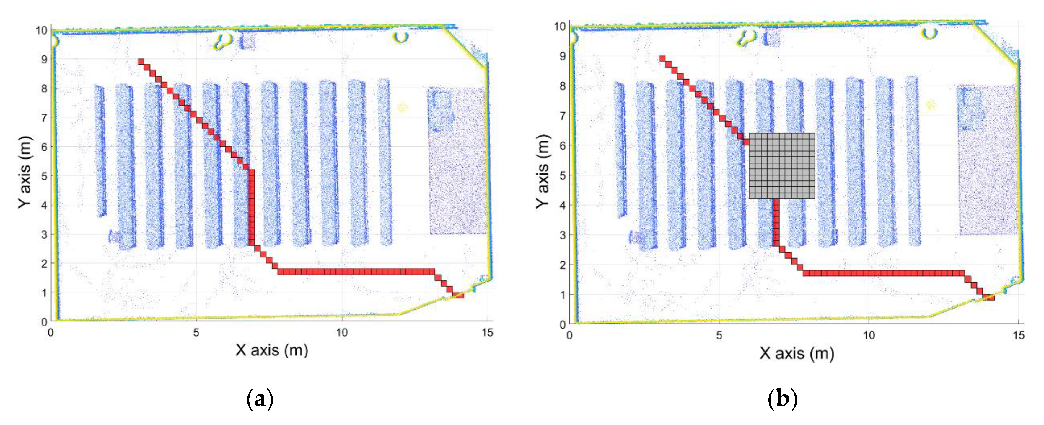
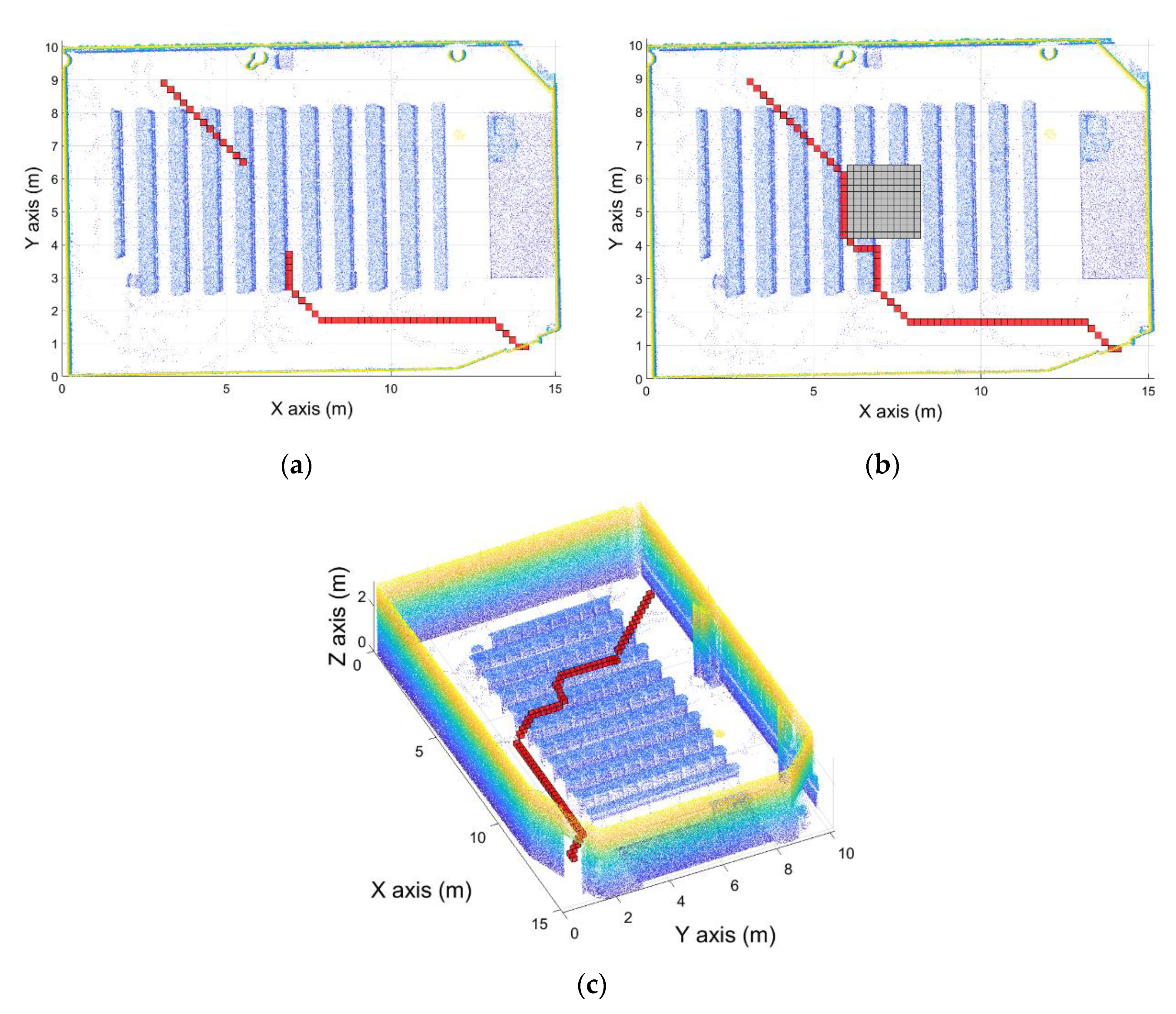
2.2. Path Planning
| Algorithm 2 Path Planning Algorithm |
|
3. Result and Discussion
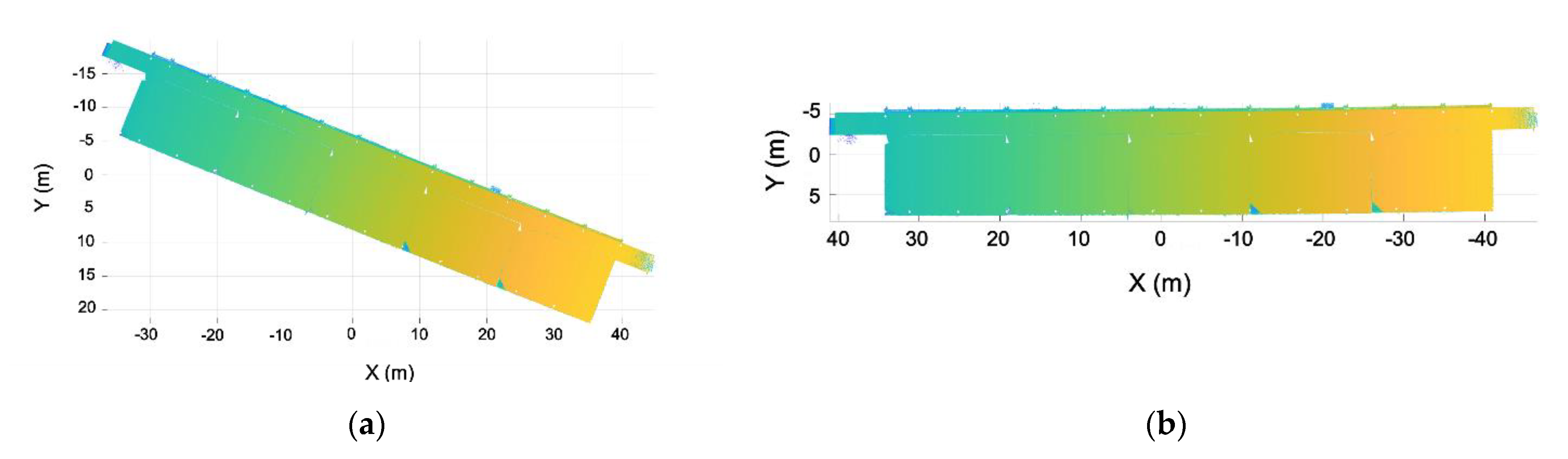
3.1. Case Study
3.2. Results
4. Conclusions
- The pre-processing step segments the entire point cloud into rooms, and each room is discretized, calculating the navigation map for each one using the doors as the target position.
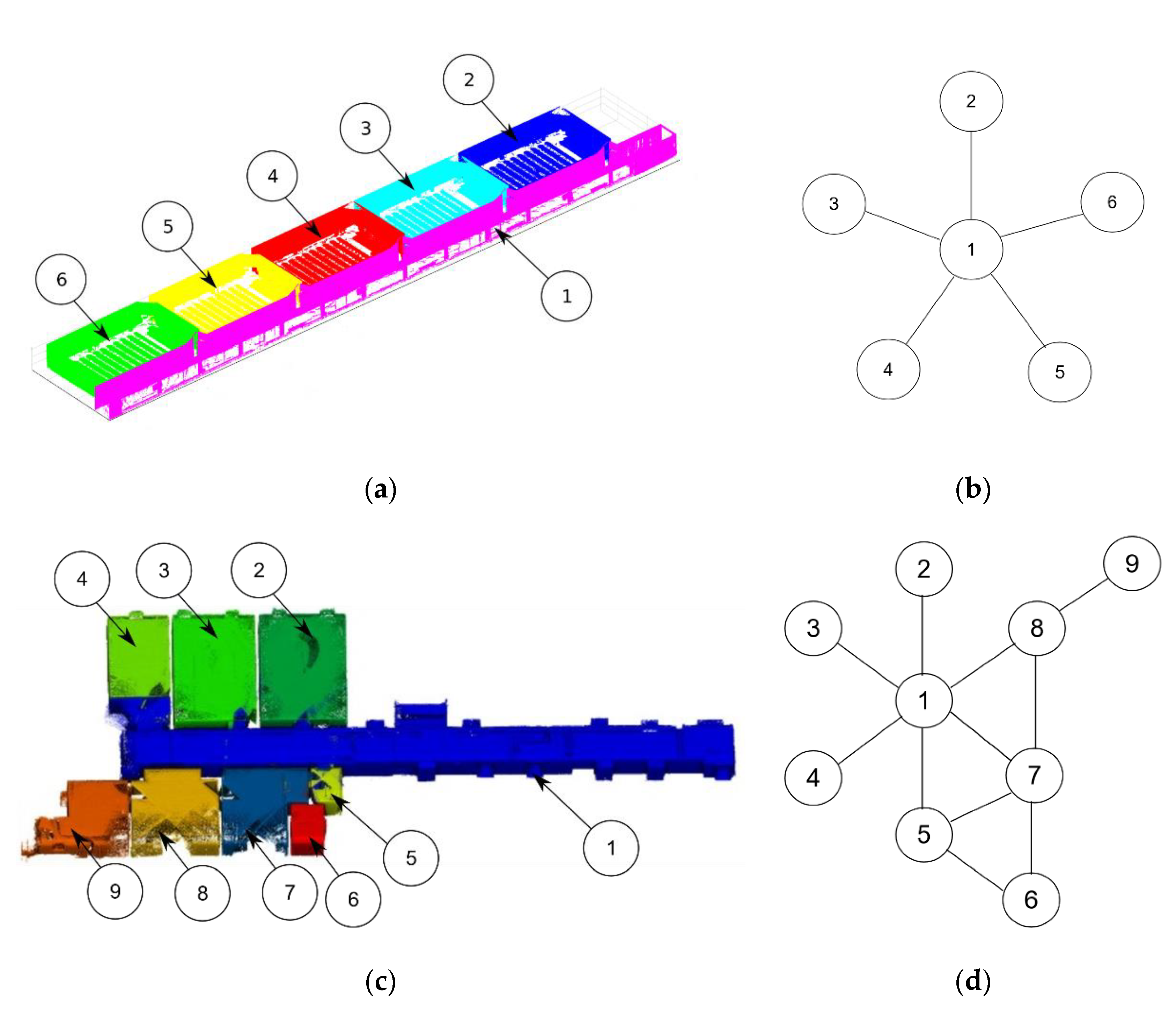
- The algorithm calculates the navigation graph of the building where the system is going to navigate.
- The path planning algorithm uses the navigation graph to calculate the rooms that the UAV has to cross in order to go from an initial point in one room to a final point in another one.
- The path planner algorithm also uses the navigation map generated in the pre-processing step to calculate the path, making this calculation in real time.
Author Contributions
Funding
Institutional Review Board Statement
Informed Consent Statement
Data Availability Statement
Conflicts of Interest
References
- Greenwood, W.W.; Lynch, J.P.; Zekkos, D. Applications of UAVs in Civil Infrastructure. J. Infrastruct. Syst. 2019, 25, 04019002. [Google Scholar] [CrossRef]
- Seo, J.; Duque, L.; Wacker, J.P. Field Application of UAS-Based Bridge Inspection. Transp. Res. Rec. J. Transp. Res. Board 2018, 2672, 72–81. [Google Scholar] [CrossRef]
- Ellenberg, A.; Kontsos, A.; Moon, F.; Bartoli, I. Bridge related damage quantification using unmanned aerial vehicle imagery. Struct. Control. Health Monit. 2016, 23, 1168–1179. [Google Scholar] [CrossRef]
- Remondino, F.; Barazzetti, L.; Nex, F.C.; Scaioni, M.; Sarazzi, D. UAV Photogrammetry for Mapping and 3d Modeling–Current Status And Future Perspectives. ISPRS Int. Arch. Photogramm. Remote. Sens. Spat. Inf. Sci. 2012, 25–31. [Google Scholar] [CrossRef] [Green Version]
- Teng, G.E.; Zhou, M.; Li, C.; Wu, H.H.; Li, W.; Meng, F.R.; Zhou, C.C.; Ma, L. Mini-UAV Lidar for Power Line Inspection. ISPRS Int. Arch. Photogramm. Remote. Sens. Spat. Inf. Sci. 2017, 2, 297–300. [Google Scholar] [CrossRef] [Green Version]
- Márquez, F.P.G.; Ramírez, I.S.; Segovia, I. Condition monitoring system for solar power plants with radiometric and thermographic sensors embedded in unmanned aerial vehicles. Meas. J. Int. Meas. Confed. 2019, 139, 152–162. [Google Scholar] [CrossRef] [Green Version]
- Sony, S.; LaVenture, S.; Sadhu, A. A literature review of next-generation smart sensing technology in structural health monitoring. Struct. Control. Health Monit. 2019, 26, e2321. [Google Scholar] [CrossRef]
- Ikeda, T.; Yasui, S.; Fujihara, M.; Ohara, K.; Ashizawa, S.; Ichikawa, A.; Okino, A.; Oomichi, T.; Fukuda, T. Wall contact by octo-rotor UAV with one DoF manipulator for bridge inspection. In Proceedings of the 2017 IEEE/RSJ International Conference on Intelligent Robots and Systems (IROS), Vancouver, BC, Canada, 24–28 September 2017; pp. 5122–5127. [Google Scholar]
- Sanchez-Cuevas, P.J.; Ramon-Soria, P.; Arrue, B.; Ollero, A.; Heredia, G. Robotic System for Inspection by Contact of Bridge Beams Using UAVs. Sensors 2019, 19, 305. [Google Scholar] [CrossRef] [Green Version]
- Han, H.; Wang, J.; Wang, J.; Tan, X. Performance Analysis on Carrier Phase-Based Tightly-Coupled GPS/BDS/INS Integration in GNSS Degraded and Denied Environments. Sensors 2015, 15, 8685–8711. [Google Scholar] [CrossRef] [Green Version]
- González-Desantos, L.; Martínez-Sánchez, J.; González-Jorge, H.; Navarro-Medina, F.; Arias, P. UAV payload with collision mitigation for contact inspection. Autom. Constr. 2020, 115, 103200. [Google Scholar] [CrossRef]
- Potorti, F.; Palumbo, F.; Crivello, A. Sensors and Sensing Technologies for Indoor Positioning and Indoor Navigation. Sensors 2020, 20, 5924. [Google Scholar] [CrossRef] [PubMed]
- Deng, H.; Fu, Q.; Quan, Q.; Yang, K.; Cai, K.-Y. Indoor Multi-Camera-Based Testbed for 3-D Tracking and Control of UAVs. IEEE Trans. Instrum. Meas. 2020, 69, 3139–3156. [Google Scholar] [CrossRef]
- Xin, C.; Wu, G.; Zhang, C.; Chen, K.; Wang, J.; Wang, X. Research on Indoor Navigation System of UAV Based on LIDAR. In Proceedings of the 2020 12th International Conference on Measuring Technology and Mechatronics Automation (ICMTMA), Phuket, Thailand, 28–29 February 2020; pp. 763–766. [Google Scholar]
- Chen, Y.; Gonzalez-Prelcic, N.; Heath, R.W. Collision-Free UAV Navigation with a Monocular Camera Using Deep Reinforcement Learning. In Proceedings of the 2020 IEEE 30th International Workshop on Machine Learning for Signal Processing (MLSP), Espoo, Finland, 21–24 September 2020. [Google Scholar]
- Moussa, M.; Zahran, S.; Mostafa, M.; Moussa, A.; El-Sheimy, N.; Elhabiby, M. Optical and Mass Flow Sensors for Aiding Vehicle Navigation in GNSS Denied Environment. Sensors 2020, 20, 6567. [Google Scholar] [CrossRef] [PubMed]
- Youn, W.; Ko, H.; Choi, H.S.; Choi, I.H.; Baek, J.-H.; Myung, H. Collision-free Autonomous Navigation of a Small UAV Using Low-cost Sensors in GPS-denied Environments. Int. J. Control Autom. Syst. 2020, 1–16. [Google Scholar] [CrossRef]
- Aggarwal, S.; Kumar, N. Path planning techniques for unmanned aerial vehicles: A review, solutions, and challenges. Comput. Commun. 2020, 149, 270–299. [Google Scholar] [CrossRef]
- Dijkstra, E.W. A note on two problems in connection with graphs. Numer. Math. 1959, 1, 269–271. [Google Scholar] [CrossRef] [Green Version]
- Yang, L.; Qi, J.; Xiao, J.; Yong, X. A literature review of UAV 3D path planning. In Proceeding of the 11th World Congress on Intelligent Control and Automation, Shenyang, China, 29 June–4 July 2014; pp. 2376–2381. [Google Scholar] [CrossRef]
- Iacono, M.; Sgorbissa, A. Path following and obstacle avoidance for an autonomous UAV using a depth camera. Robot. Auton. Syst. 2018, 106, 38–46. [Google Scholar] [CrossRef]
- Valenti, F.; Giaquinto, D.; Musto, L.; Zinelli, A.; Bertozzi, M.; Broggi, A. Enabling Computer Vision-Based Autonomous Nav-igation for Unmanned Aerial Vehicles in Cluttered GPS-Denied Environments. In Proceedings of the 2018 21st International Conference on Intelligent Transportation Systems (ITSC), Maui, HI, USA, 4–7 November 2018; pp. 3886–3891. [Google Scholar]
- Lakas, A.; Belkhouche, B.; Benkraouda, O.; Shuaib, A.; Alasmawi, H.J. A Framework for a Cooperative UAV-UGV System for Path Discovery and Planning. In Proceedings of the 2018 International Conference on Innovations in Information Technology (IIT), Al Ain, UAE, 18–19 November 2018; pp. 42–46. [Google Scholar]
- Yan, W.; Culp, C.; Graf, R. Integrating BIM and gaming for real-time interactive architectural visualization. Autom. Constr. 2011, 20, 446–458. [Google Scholar] [CrossRef]
- Peralta, F.; Arzamendia, M.; Gregor, D.; Reina, D.; Toral, S. A Comparison of Local Path Planning Techniques of Autonomous Surface Vehicles for Monitoring Applications: The Ypacarai Lake Case-study. Sensors 2020, 20, 1488. [Google Scholar] [CrossRef] [Green Version]
- Korkmaz, M.; Durdu, A. Comparison of optimal path planning algorithms. In Proceedings of the 2018 14th International Conference on Advanced Trends in Radioelecrtronics, Telecommunications and Computer Engineering (TCSET), Slavske, Ukraine, 20–24 January 2018; pp. 255–258. [Google Scholar]
- Huang, X.; Cao, Q.; Zhu, X. Mixed path planning for multi-robots in structured hospital environment. J. Eng. 2019, 2019, 512–516. [Google Scholar] [CrossRef]
- Maoudj, A.; Hentout, A. Optimal path planning approach based on Q-learning algorithm for mobile robots. Appl. Soft Comput. 2020, 97, 106796. [Google Scholar] [CrossRef]
- Hernández-Mejía, C.; Vázquez-Leal, H.; Sánchez-González, A.; Corona-Avelizapa, Á. A Novel and Reduced CPU Time Modeling and Simulation Methodology for Path Planning Based on Resistive Grids. Arab. J. Sci. Eng. 2019, 44, 2321–2333. [Google Scholar] [CrossRef]
- Ambroziak, T.; Malesa, A.; Kostrzewski, M. Analysis of multicriteria transportation problem connected to minimization of means of transport number applied in a selected example. WUT J. Transp. Eng. 2018, 123, 5–20. [Google Scholar] [CrossRef]
- Dang, T.; Tranzatto, M.; Khattak, S.; Mascarich, F.; Alexis, K.; Hutter, M. Graph-based subterranean exploration path planning using aerial and legged robots. J. Field Robot. 2020. [Google Scholar] [CrossRef]
- Li, H.; Savkin, A.V.; Vucetic, B. Autonomous Area Exploration and Mapping in Underground Mine Environments by Unmanned Aerial Vehicles. Robotica 2020, 38, 442–456. [Google Scholar] [CrossRef]
- Ltd, G. ZEB-REVO Laser Scanner. Available online: https://download.geoslam.com/docs/zeb-revo/ZEB-REVOUserGuideV3.0.0.pdf (accessed on 3 November 2020).
- González-Desantos, L.M.; Martínez-Sánchez, J.; González-Jorge, H.; Arias, P. Path planning for indoor contact inspection tasks with UAVS. Int. Arch. Photogramm. Remote Sens. Spat. Inf. Sci. 2020, 43, 345–351. [Google Scholar] [CrossRef]
- Díaz-Vilariño, L.; Verbree, E.; Zlatanova, S.; Diakite, A. Indoor modelling from SLAM-based laser scanner: Door detection to envelope reconstruction. Int. Arch. Photogramm. Remote Sens. Spat. Inf. Sci. 2017, 42, 345–352. [Google Scholar] [CrossRef] [Green Version]
- Fischler, M.A.; Bolles, R.C. Random sample consensus: A paradigm for model fitting with applications to image analysis and automated cartography. Commun. ACM 1981, 24, 381–395. [Google Scholar] [CrossRef]
- González-Desantos, L.M.; Díaz-Vilariño, L.; Balado, J.; Martínez-Sánchez, J.; González-Jorge, H.; Sánchez-Rodríguez, A. Autonomous Point Cloud Acquisition of Unknown Indoor Scenes. ISPRS Int. J. Geo-Inf. 2018, 7, 250. [Google Scholar] [CrossRef] [Green Version]


| N. Path | Initial Pos. (m) | Final Pos. (m) | Vec. Dir. | Time (s) | N. Waypoints. |
|---|---|---|---|---|---|
| 1 | [−27.9, 5.85, −0.8] | [4.2, 2.3, 1] | [−1, 0, 0] | 0.008745 | 345 |
| 2 | [−13.5, 5.85, −0.8] | [19.4, 2.3, 1] | [−1, 0, 0] | 0.006259 | 340 |
| 3 | [1.2, 5.85, −0.8] | [−10.6, 2.3, 1] | [−1, 0, 0] | 0.00851 | 342 |
| 4 | [17.2, 5.85, −0.8] | [−25.5, 2.3, 1] | [−1, 0, 0] | 0.012885 | 263 |
| 5 | [32, 5.85, −0.8] | [−40.6, 2.3, 1] | [−1, 0, 0] | 0.006533 | 415 |
| 6 | [−27.9, 5.85, −0.8] | [18.4, 2.5, 1] | [1, 0, 0] | 0.008942 | 303 |
| 7 | [−13.5, 5.85, −0.8] | [33.5, 3, 1] | [1, 0, 0] | 0.005645 | 289 |
| 8 | [17.2, 5.85, −0.8] | [3.4, 3, 1] | [1, 0, 0] | 0.009818 | 151 |
| 9 | [17.2, 5.85, −0.8] | [−11.5, 3, 1] | [1, 0, 0] | 0.005481 | 239 |
| 10 | [32, 5.85, −0.8] | [−26.7, 3, 1] | [1, 0, 0] | 0.006902 | 377 |
| N. Path | Time A* (s) | Time Modified A* (s) | |
|---|---|---|---|
| 1 | 1.550767 | 0.008745 | 177.33 |
| 2 | 1.576993 | 0.006259 | 251.96 |
| 3 | 1.416444 | 0.00851 | 166,44 |
| 4 | 1.538592 | 0.012885 | 119.41 |
| 5 | 1.591487 | 0.006533 | 243.61 |
| 6 | 1.411514 | 0.008942 | 250.05 |
| 7 | 1.522057 | 0.005645 | 269.63 |
| 8 | 1.339394 | 0.009818 | 136.42 |
| 9 | 1.509533 | 0.005481 | 275.41 |
| 10 | 1.647614 | 0.006902 | 238.72 |
Publisher’s Note: MDPI stays neutral with regard to jurisdictional claims in published maps and institutional affiliations. |
© 2021 by the authors. Licensee MDPI, Basel, Switzerland. This article is an open access article distributed under the terms and conditions of the Creative Commons Attribution (CC BY) license (http://creativecommons.org/licenses/by/4.0/).
Share and Cite
González de Santos, L.M.; Frías Nores, E.; Martínez Sánchez, J.; González Jorge, H. Indoor Path-Planning Algorithm for UAV-Based Contact Inspection. Sensors 2021, 21, 642. https://doi.org/10.3390/s21020642
González de Santos LM, Frías Nores E, Martínez Sánchez J, González Jorge H. Indoor Path-Planning Algorithm for UAV-Based Contact Inspection. Sensors. 2021; 21(2):642. https://doi.org/10.3390/s21020642
Chicago/Turabian StyleGonzález de Santos, Luis Miguel, Ernesto Frías Nores, Joaquín Martínez Sánchez, and Higinio González Jorge. 2021. "Indoor Path-Planning Algorithm for UAV-Based Contact Inspection" Sensors 21, no. 2: 642. https://doi.org/10.3390/s21020642