Article

ROBINA: Rotational Orbit-Based Inter-Node Adjustment for Acoustic Routing Path in the Internet of Underwater Things (IoUTs)

1
Department of Computer Science, Lahore Campus, CUI, Lahore 54000, Punjab, Pakistan
2
Department of Computer Science, University of Sahiwal, Sahiwal 57000, Punjab, Pakistan
3
Department of Computer Science, University of Okara, Okara 56300, Punjab, Pakistan
4
Department of Computer Science, Sahiwal Campus, CUI, Sahiwal 57000, Punjab, Pakistan
5
Department of Computre Engineering, University of Engineering and Technology, UET, Texila 47080, Punjab, Pakistan
6
Electrical and Computer Engineering, University of Windsor, Windsor, ON N9B 3P4, Canada
7
College of Electronics and Convergence Engineering, Kyung Hee University, Yongin 446-901, Korea
*
Author to whom correspondence should be addressed.
Sensors 2021, 21(17), 5968; https://doi.org/10.3390/s21175968
Submission received: 5 July 2021 / Revised: 22 August 2021 / Accepted: 23 August 2021 / Published: 6 September 2021
(This article belongs to the Special Issue Wireless Sensor Networks for Water and Environmental Monitoring)

Abstract

:
The Internet of Underwater Things (IoUTs) enables various underwater objects be connected to accommodate a wide range of applications, such as oil and mineral exportations, disaster detection, and tracing tracking systems. As about 71% of our earth is covered by water and one-fourth of the population lives around this, the IoUT expects to play a vital role. It is imperative to pursue reliable communication in this vast domain, as human beings’ future depends on water activities and resources. Therefore, there is a urgent need for underwater communication to be reliable, end-to-end secure, and collision/void node-free, especially when the routing path is established between sender and sonobuoys. The foremost issue discussed in this area is its routing path, which has high security and bandwidth without simultaneous multiple reflections. Short communication range is also a problem (because of an absence of inter-node adjustment); the acoustic signals have short ranges and maximum-scaling factors that cause a delay in communication. Therefore, we proposed Rotational Orbit-Based Inter Node Adjustment (ROBINA) with variant Path-Adjustment (PA-ROBINA) and Path Loss (PL-ROBINA) for IoUTs to achive reliable communication between the sender and sonobuoys. Additionally, the mathematical-based path loss model was discussed to cover the PL-ROBINA strategy. Extensive simulations were conducted with various realistic parameters and the results were compared with state-of-the-art routing protocols. Extensive simulations proved that the proposed routing scheme outperformed different realistic parameters; for example, packet transmission 45% increased with an average end-to-end delay of only 0.3% respectively. Furthermore, the transmission loss and path loss (measured in dB) were 25 and 46 dB, respectively, compared with other algorithms, for example, EBER2 54%, WDFAD-BDR 54%, AEDG 49%, ASEGD 55%, AVH-AHH-VBF 54.5%, and TANVEER 39%, respectively. In addition, the individual parameters with ROBINA and TANVEER were also compared, in which ROBINA achieved a 98% packet transmission ratio compared with TANVEER, which was only 82%.

1. Introduction

The Internet of Underwater things (IoUTs) involves a group of sensor nodes that gather data from different sensors placed in the ocean’s depths to further transfer them towards the positioned devices at the external level through a network of midway nodes. The IoUTs consists of sensors and relay nodes that use acoustic mediums for communication. It can support various applications such as underwater tracking, climate exposure and recording, oceanographic information, pollution detection, underwater surveillance, navy defense systems, offshore exploration, and disaster prevention. As one-third of our population is surrounded by water and millions of people live within 100 km of the coastal area [1], the IoUTs will play a vital role.
State-of-the-art literature discourses the problems and limitations that interrupt the IoUTs’ effectiveness, including bandwidth limitation, high energy consumption, inadequate energy resources, efficient routing, and increased distribution cost [2]. Dynamic topology and water current are fundamental parameters for controlling the mobility factor inside the underwater field. The deployment of nodes before and after the experiment are quite different. Therefore, it is difficult to predict which node is inactive/alive/dead in shallow and deep water. Basically, the dead nodes are the gaps of nodes when the communication is near to the destination and is overburdened. When these nodes are found frequently in network size, the void nodes become void regions that isolate some part of the network. The main reason for this event is the absence of the candidate nodes that take responsibility for those nodes that are dying or are going to die. In addition, compared to Terrestrial Wireless Sensor Networks (TWSNs), identifying the localization of nodes is also difficult as radio signals do not work in underwater scenarios. For this reason, one of the best substitutes is the use of acoustics links. Moreover, energy in batteries or other means is limited and difficult to replace or re-charge in underwater scenarios.
In the literature, many routing schemes and algorithms have been reported to minimize the energy consumption of the nodes and identify dead nodes [3,4]. The dead nodes are those nodes that are not able to deliver the data to sonobuoys. For quick data delivery, many routing and flooding schemes use the shortest path and routing tables, angle-based flooding, the three-hop reliability model, watchman-based flooding, depth and location-based routing, pressure, and cluster/subnet-based approaches [5,6,7,8]. As nodes around the sonobuoys suffer, and the entire traffic load can die early, we propose the internodes adjustment mechanism for providing an alternative route by following the greedy forwarding approach to recover the data from the dead nodes. At the same time, Path Adjustment (PA) is perfomed by following the rotational orbit-based shape for alternative ways, collectively called Rotational Orbit-Based Inter-Node Adjustment (ROBINA).
Moreover, its two sub-variants: Path-Adjustment (PA-ROBINA) and Path Loss (PL-ROBINA), were proposed in this article. The ROBINA uses geographic energy-efficient data communication while PA-ROBINA provides proper path adjustment to bypass the dead nodes to discern the Immediate Available Forwarder Node (IAFN) after dead nodes. In addition, the PL-ROBINA uses the path loss transmission model to divert the path according to desired (IAFN). Moreover, the mode of operation is based upon the inter node adjustment mecahnisam. The relationship between rotation orbit and path selection is basically interlinked with each other. It is because of the rotation orbit-based pathway is used to find new node in the communication range. The path selection will automatically adjusted with the position of new finding node.
The mathematical-based formulas were introduced to create a path with a maximum rotation covering the main proposed approach, ROBINA. The possible model of this scheme is shown in Figure 1, where the occurrence of dead nodes is rescued through inter-nodes adjustment, and an alternate routing path is provided by a rotational orbit-based path as mentioned earlier.
Furthermore, the data received from dead nodes are covered by the internodes as these are responsible for transferring the data to sonobuoys. In case of data delivery failure to the internodes, the nearest sonobuoys automatically take the data using a first-come, first-served approach. In this regard, the PA-ROBINA and PL-ROBINA can provide a smooth communication path towards the sonobuoys and ensure that the data from the nodes (dead nodes) can be delivered to the destination.
In addition, the atomic shape-based data gathering routing protocol is already added to our contribution in the literature [9,10] for efficient delay and data gathering purposes. For this purpose, Autonomous Underwater Vehicles (AUV) are deployed along with member and gateway nodes [11]. Underwater AUVs are responsible for transferring the data to the derived destination without using internode adjustment; however, the long, unnecessary propagation delay occurs [12]. In addition, the extra consumption of energy and chances of packet dropping also make their impact [13]. Ultimately, the performance of the routing protocol is compromised. ROBINA takes this scenrion as an advantage for introducing inter-nodes adjustment between void holes rather than using AUVs.
Although the Potential Forwarder Node (PFN) can be replaced and substituted for inter-node adjustment for some reason, the establishment of the path, long routing cache, and criteria of selection of the PFN can be responsible for not outperforming in a well-disciplined manner. The dependency in EBER2 [14] (that uses the concept of PFN) also takes different transmissions for data delivery (which is not required; it is because we usually encourage more transmission in the vehicular network, ad hoc network, and for terrestrial networks). ROBINA does not use a different transmission; data delivery is performed through internode adjustment. Otherwise, packets will be dropped. Though depth is the most trustable factor in an underwater environment, it is not constant in oceans due to the dynamic nature of water surfaces. Therefore, line of sight direction, Zig-Zag path, and depth-based information followed by the shortest path cannot be performed well. As the underwater environmenmt is based upon the medium to large-scale networks, to cover this area with minimum energy consumption, there is a dire need to establish a path strategy that covers the area with minimum EC impact.
Extensive simulations were conducted, where the state-of-the-art routing protocols like AVH-AHH-VBF [9], ASEDG [11], AEDG [13], EBER2 [14], and WDFAD-DBR [15] were compared. It was demonstrated that the ROBINA outperforms affordable EC, minimum E2E delay, and high PDR. Our suggested method, ROBINA, and its co-variant PL-ROBINA employ Immediate Available Forwarder Nodes (IAFN). The basic function of using IAFN rescues the routing path when it is established between two nodes. The relay nodes are randomly deployed inside the network that plays a part-and-parcel role to make the communication reliable and smoothly proceed the process of data packet delivery. From Figure 1, the (IAFN) near-relay nodes are available for communication as the subistiution for dead nodes. Relay nodes basically provide the information about these IAFN with gateways for established communication between forwarder nodes and sink through the selected path.
Our Contributions. After introducing the idea underlines for rotation of path and its adjustment against various parameters, we proposed a rotational-based scheme that accordingly selects forwarder nodes in its routing path by ROBINA. We used Path Adjustment and Path Loss, called PA-ROBINA and PL-ROBINA, respectively for the adjustment and path loss mechanism. The PA-ROBINA is basically used for adjustment of the path based on the provided information by relay nodes and IAFN. As in IoUT, the nodes can only be remotely accessed, and unmanned effort is required for this environment to make the path consistent and reliable for acoustic IoT devices. We used the path loss function to detect the void nodes and rotate the path with the following ROBINA, called PL-ROBINA. The ROBINA and its co-variants work with IAFN, which is the core mechanism of internodes adjustment. The criteria to choose the IAFN was provided, while the mathematical model was also produced to select the optimal IAFN with the help of Urick’s Model and Thorp’s Formula. The contributions can be summarized as follows:
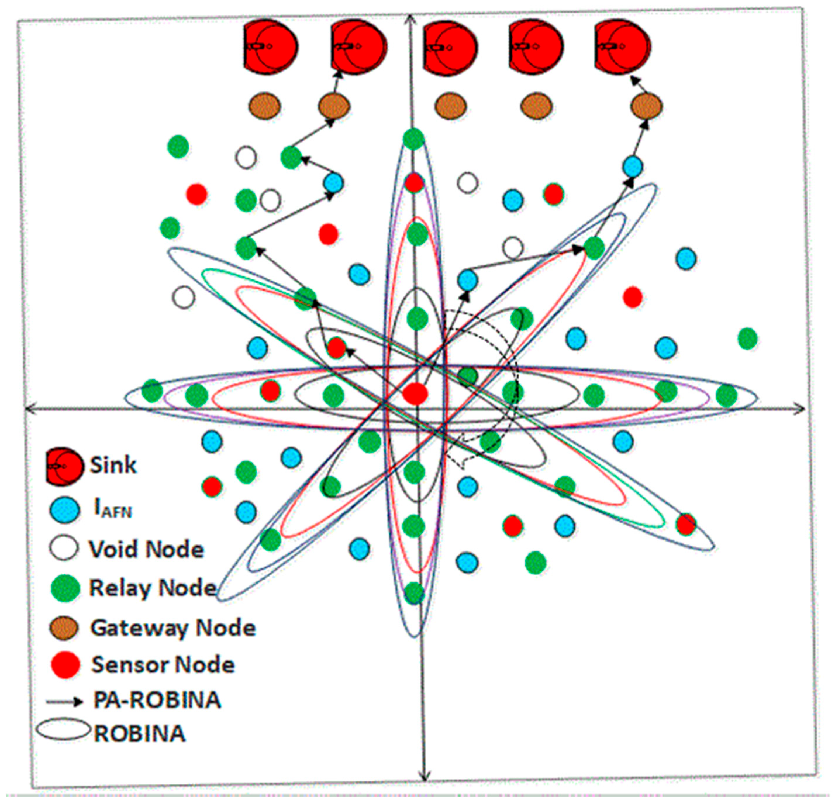
We presented the ROBINA for inter-node modifications in all possible directions following path rotations until all nodes are designated for communication and are within the radius of the rotated path.
We also analyzed the relay nodes quantity that is selected under the criteria of path rotation and adjusted its position by PA-ROBINA. It also uses the IAFN function and Parity bit-based flags to choose nodes that are closest to the destinations.
We opted for and reformulated the ambient noise-reduction solution using the Urick’s Model for acoustic signals, and absorption loss factor by Thorp’s Formula, that modeled continuous Power Spectral Density (PSD) and Colored Gaussian Statistics (CGS). All these work for PL-ROBINA.
We evaluated the first rotational orbit-based proposed scheme’s performance by comparing it with state-of-the-art benchmark schemes under different parameters of transmission loss, throughput, number of dead nodes, and etc.
The rest of the work is organized as follows. We reviewed state-of-the-art literature in Section 2 and provided the problem formulation in Section 3. Furthermore, Section 4 and Section 5 present the proposed schemes and their sub-sections. The path loss channel model is described in Section 6. Finally, the simulation results and conclusion are provided in Section 7 and Section 8, respectively.

2. Literature Review

Recently, the demand for the deployment of sensor networks in the underwater environment has gained significant attention in the networking domain with unique features and continuous sensing movement.
A protocol for the IoUTs, namely Energy-Balanced Efficient and Reliable Routing (EBER2) is discussed in [14] to balance energy and achieve reliability. EBER2 deliberates enduring significance and the number of PFN transmission choices divided among the power levels to enhance energy effectiveness. The protocol allows forwarders to adaptively control their communication according to the utmost node in the neighbor list of the network. To reduce the duplication of packets, residual energy, PFNs, and their depths are compared among the neighbors. Moreover, two sinks are deployed at high-density traffic areas to reduce network latency. The study results show that EBER2 has lowered energy consumption and identical packets with low packet delivery ratios compared with the Weighting Depth and Forwarding Area Division-Depth Based Routing (WDFAD-DBR) protocol [15]. The WDFAD-DBR mechanism considers the depth of the next forwarding node, through which it avoids void holes. Multiple IoUTs schemes have been designed to prevent voids holes, including AVH-AHH-VBF and SM-AHH-VBF [9]. These schemes’ main concern is to raise the lifespan of the sensor network system with low energy consumption. The study results show that the proposed methods outperform high energy consumption with an end-to-end interruption in packet transfer, average packet delivery ratio, and average propagation distance compared with the baseline solution.
Another issue is imbalance of energy consumption that degrades the overall performance of sensor-based networks with high data-traffic flow between intermediate nodes [3]. Many researchers have worked for efficient energy consumption and data-traffic distribution to reduce the intermediate node’s packet forwarding ratio. For this purpose, an Energy Grade (EG) and load-balance-distributed corona were proposed in [10]. A corona-deprived EG and a corona deprived of Depth Adjustment (DA)-enabled schemes are proposed to allocate the flow of data traffic nodes for effective energy distribution. The dynamic alteration of the communication range in the initial method supports the reduction of data load. Both EG and DA work to allocate data traffic for equal distribution of energy.
IoUTs face serious packet delivery problems, packet loss, and collisions because of the solid placement of the sensing nodes in severe underwater environments. The retransmission of the packets causes a lot of energy consumption and interruption, and delays in packet delivery. A framework was proposed in [4] to minimize energy loss, maximize throughput, and improve the network’s lifetime. A three-dimensional 3D acoustic scenario [5] usually works with a distributed sink that is not static in network stability, packet loss analysis, and lifetime. Furthermore, the proposed framework was compared with prevailing techniques like Mobicast and iAMCTD protocols that pointed out node compactness in the network with an adaptation of varying depth consequences and DA in low energy consumption reduces retransmission and improved throughput [8]. The proposed framework delivers an improved performance for real-time interruption-based applications over the current mechanisms.
The major challenge of the IoUTs is sending data towards the sink stations; due to the continuous movement of the nodes, it becomes difficult to transfer data. In order to overcome this problem, we make the orbit-based routing path in our proposed scheme with supporting thories listed in [16,17] and Opportunistic Routing Protocols (ORPs) [18,19] are examined to expand performance with a dynamic selection of one best forwarding device from the other. Location-Based Opportunistic Routing Protocols (LBORPs) are recognized and identified to perform better using knowledge for dynamic selection of forwarder devices through their location and route message packets to the receiver [7]. The functioning of location-focused routing protocols is studied to perform well in IoUTs atmospheres. Hence, these location-based protocols decrease performance in IoUTs networks due to communication ejects or holes (sometimes called void holes and region) [5]. The researchers discussed the working of LBORPs communication voids in IoUTs along with their problems and disadvantages. The first LBORP is VBF and the second one is HH-VBF, which are analyzed where VBF establishes a simulated vector pipe for routing among source and receiver sink nodes, only those in the virtual vector. Whereas, in the HH-VBF protocol, each node uses different virtual pipes and during each time of transmission the direction of the virtual pipe changes. A comparison of both VBF and HH VBF protocols was performed to analyze the performance of both protocols, and the networks consequently received better performance without communication void holes. Routing issues and challenges related to the IoUTs were identified to assist the scholars in developing and deploying efficient IoUTs routing protocols with multiple communication holes. Further the estimated distance based approaches are discussed [20,21] in which the routing path and its calculation from sink.
Another routing technique called TANVEER, with its three sub-sections, LBA-TANVEER, DPD-TANVEER, and BIN-TANVEER, experimented with IoUTs [22]. These schemes are based on triangular calculations to bypass empty regions and follow the smooth route towards destinations. The author used a straightforward approach to mitigate the blank nodes inside the routing path. The experimental results suggested that the TANVEER and BIN-TANVEER secured satisfied marks against a fraction of empty regions.

3. Problem Formulations

Two out of four routing techniques proposed different routing paths that directly connect the source and sinks through intermediate, relay, and forwarder nodes. The probability of packet losses, node failure, energy tax (extra), and inefficient data gathering in these schemes is common. Furthermore, the direct path through mediators’ nodes is an old technique in which EBER2, WDFAD-DBR, and AVH-AHH-VBF are inline. With reference to their simulation, unsatisfactory results are achieved. Moreover, the AEDG and ASEDG both introduce the atomic shape path for relay nodes and sinks. Still, it is not rotational, so there is a need to design a routing path that is shortest in length and covers the parameters mentioned above. In our proposed work, there was some consideration because of our focus on the avoidance of void nodes by introducing inter-node adjustment and providing alternative paths via rotational orbit-based shapes (as orbits are much denser then atomic and elliptical shapes and cover a larger area [11,13]). The first consideration is: (i) every node has its localization information, (ii) symmetric communication was assumed between two nodes, for example, ‘i’ and ‘j’, (iii) sinks can receive multiple buckets at the same time, (iv) the vertical direction in water was mostly not considered, but due to water current, the horizontal direction was considered, (v) dead nodes were near the sinks called Sonobuoys Neighboring Nodes (SNNs), and its orbit path was considered for these SNNs when introducing inter-node adjustment (which is the proposed scheme), and (vi) if the SNNs zone is closer to the sinks, then the internode has sent the data directly without taking an alternative path to improve network throughput [19]. The major contribution of our work is as follows.
Our contribution in this regard was to make the path officially rotational (based on inter-nodes adjustment) and have orbits shape, not atomic and elliptical [11]. It is interesting to know about atomic that its particle is itself surrounded by rotation. However, the atomic particles that move around its central point also have the shape of orbits. The major advantage of the orbit-based path covers much area as compared to atomic path and elliptical. The two-way motion described in the literature according to Heisenbergs Principle [16] is possible, in which they state that “every particle have two-way motion, first itself and other around the material in which they occupied” [20].
In addition, the orbit is larger than a circle, and quite similar to an elliptical shape; on the contrary, the atomic path is also under the umbrella of eclipse shapes. From this reference, we can say that the ancestor of these shapes (including the atomic shape path used in ASEDG [13]) of the orbit has more advantages and result-oriented features in all relative parameters.
Furthermore, the area covered by the atomic path is not much greater than the orbit path mentioned in ‘Bernoullis Equation’ [17]. It states that the area covered by its volume is always directly postponed to its ‘pressure and performance.

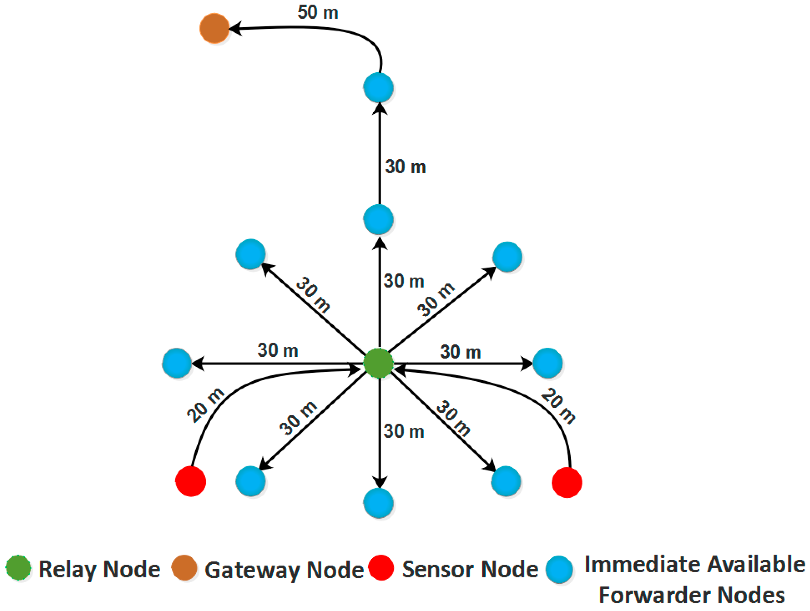
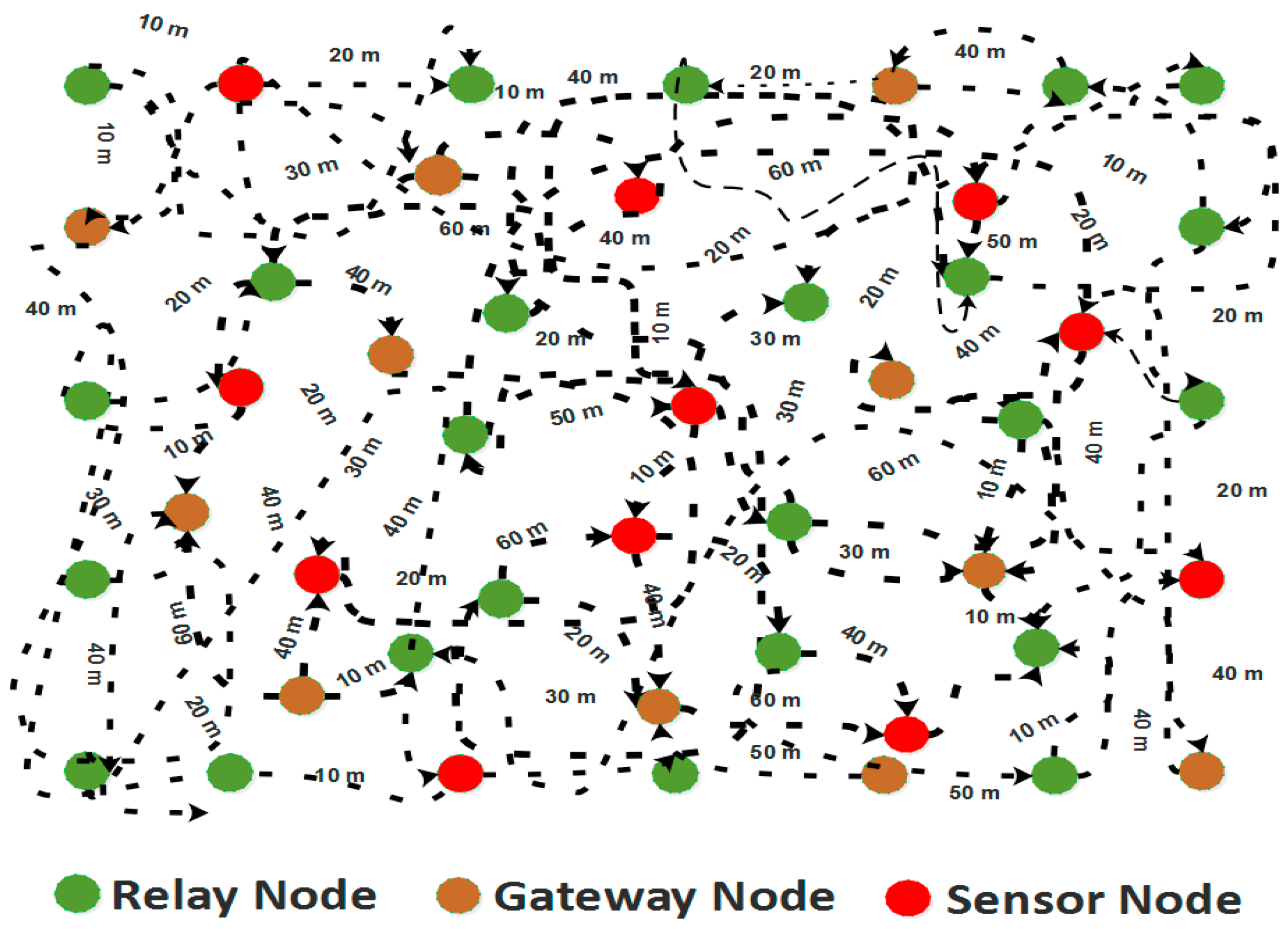
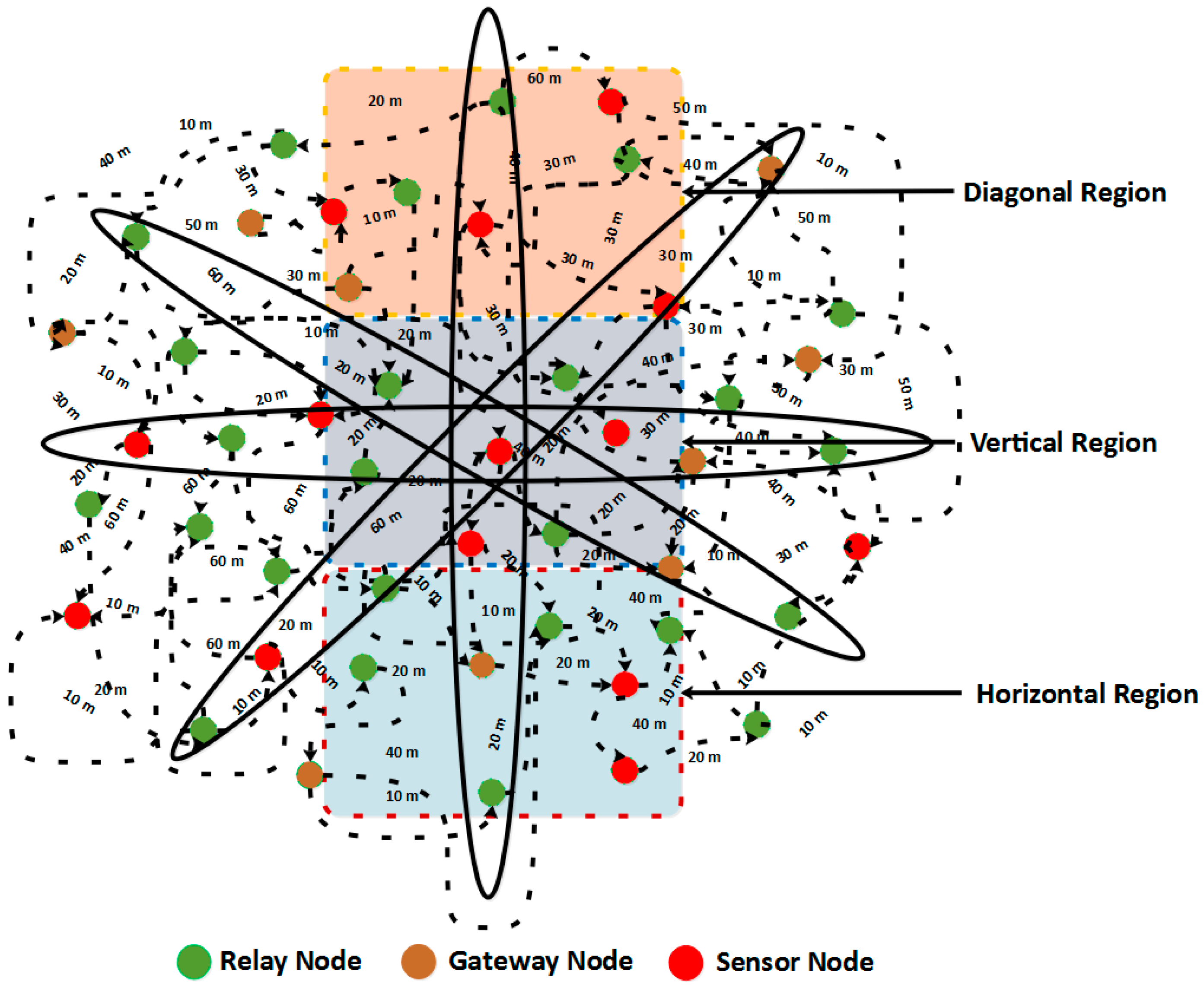
4. The Rotational Orbit Based Inter Node Adjustment (ROBINA)

The ROBINA takes the available number of nodes and its neighboring intermediate forwarding node around the sinks for reliable data transmission. Firstly, the sensor, relay, and gateway nodes are nominated and randomly deployed without the ROBINA, as shown in Figure 2. All these nodes are deployed as anchored positions, and take data information towards the sinks. In order to avoid a collision, it is assumed that one node can carry and transfer the data one packet at a time [23,24,25,26]. Due to the increased traffic volume, the empty void nodes form void regions. At that location, the internode adjusts and transmits a beacon message requesting an alternate. An alternate path based on rotational orbits is established around the SNNs. Its radius must include both the node’s void dead area and the set of neighboring nodes. It consists of multiple nodes that ensure the recovery of data with higher priority. The following mathematical expression is used to adjust internodes around SNNs in Equation (1).
A   ( A d j N i ) = E   ( N i ) (   S N N r a n g e N + f ( N i )
where f(Ni) = {1|0} (=0 for a dead state, or =1 for an alive state)
From Equation (1): the A (AdjNi) is the selected area for the proposed scheme in the network that firstly calculates the E(Ni) energy of the node and the range of ( S N N r a n g e ) where f(Ni) = {1|0} (=0 for a dead state, or =1 for an alive state). In the equation described above, we take a scenario in which node ‘i’ sends data to node ‘j’ with energy ‘E’; first, it explores the ‘Ns’ towards the ‘Sn’, then, for all nodes that wait for Packet ACKnowledgment (PACK), takes the time (t) in such a way that Nij = {ni     nj ^ Eij: AdjNi ∗ SNNs + Dn}, for orbit pathTp = n = i j ( N i j S N N s ) ,   then PACK in total time for path establishment counts the set of neighboring nodes with sink [27] as mentioned in Equation (2) with Selection Operation (Selop).
S e l o p = N s D n S n
The following equation ensures that the PACK from Node ‘i’ to ‘j’ with ‘E’ is as expected in Equation (3), where PACK is discussed in detail.
P ACK   ( N ) = j = 0 d = 1   S N N s   ( D n ) S n
Additionally, in the following section with Algorithm 1, the procedure of (IAFN) for forwarding the Beacon Message (BM) is discussed. In Algorithm 2, the detailed description of data delivery using a path adjustment mechanism is discussed. The PA-ROBINA works with internode adjustment as IAFN; while setting the internodes between the void nodes, the path will automatically adjust at that region and rescue the dead nodes. For the adjustment of the region of the path, the range of SNNs plays a role in determining which path is closer to sonobuoys so that it is easier for the path-based nodes like internodes to send the acknowledgment of the nodes that are not alive [28,29,30,31,32,33].
Moreover, the working of ROBINA for the adjustment of internode and its PA-ROBINA for setting the rotational shortest path are described in Algorithms 1 and 2, respectively. In Figure 3, the overall working of ROBINA is explained with its acoustic scenario. Usually, the scenario Underwater consists of relay nodes, sensor nodes, and gateway nodes. The relay nodes are considered as the immediate medium to pass the communication from source to destination. Gateways are present to receive data packets from relay nodes, which arepassed through the desired destination. The whole scenario is followed by an intentionally rotating path (from left to right) that is orbital in shape. The increasing trend of every orbit shape presents the refeclection of the rotating path where needed. The inside circle shows the overall rotation of the path to avoid void holes and deploy the inter-node adjustment near the SNNs. The ‘oval’ legend in Figure 4 shows the working of the orbital routing path while the ‘arrow’ denotes the straight forward path adjustment of ROBINA.
Further, the nodes closer to the destination take enough burden from the whole network communication and die early, which relay as void nodes (white in color). When these nodes are found frequently in network size, they become void regions isolated to some part of the network too. The main reason for this event is the absence of the candidate nodes responsible for those nodes that die or near death. From this reference, we introduce the idea of inter-node adjustment and formulate their path accordingly. Usually, in underwater situations, the path is horizontal, vertical, elliptical, atomic shaped, vector and depth-oriented, height and angle oriented, or etc. Due to the non-rotatable behavior of the path, all these schemes are not well performed. Therefore, a rotational-based path with an internode adjustment mechanism performs well when the area of interest is dense and shallow. The novel orbit-based path rotates with the adjacency of relay nodes, including some inter-nodes adjustment (where needed), making the communication secure and reliable.

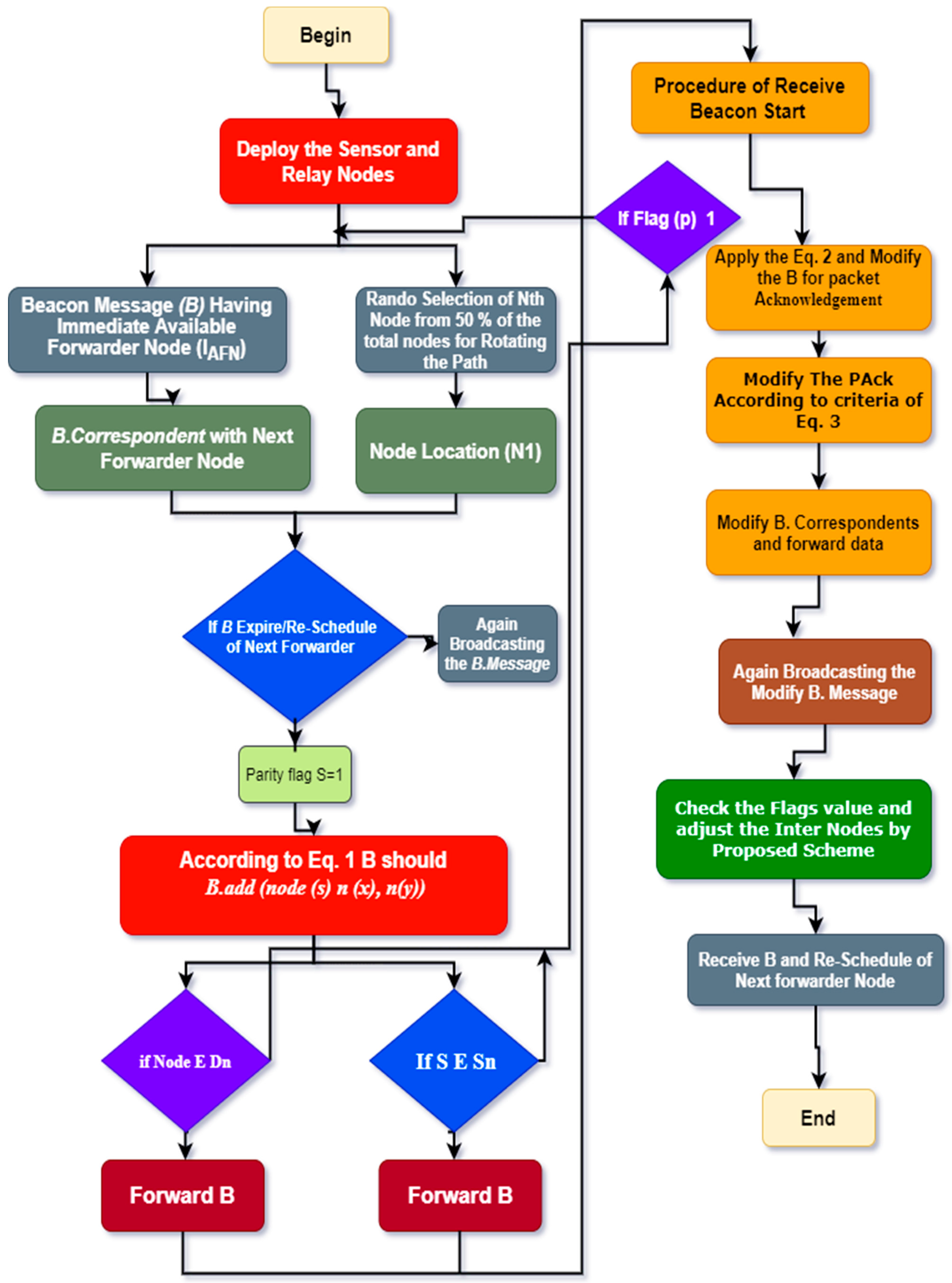
5. Description of Algorithms 1 and 2

In this section, Algorithms 1 and 2 for inter-node and path adjustment are described in detail; first, the BM are decided for forwarding and receiving acknowledgment for relay and sensor nodes, in which each ‘BM’ contains next node’s information with its correspondent coordinates to determine the location and distance of nodes. All this information is simultaneously updating in the routing table as [28,29,30].
To add the next node, the mechanism of parity flag is introduced if it is 1, then forwarder nodes with all their adjacency are added to set out the packet orientation, and ignored if it is 0. The path should be modified (due to the rotational mechanism technique used in ROBINA) if the PACK does not receive from adjacent nodes as described in Equation (2). The modified PACK is used to set down the path in the desired direction, as mentioned in Algorithm 1. The delivery of data using path adjustment only considers the next forwarder nodes and their re-scheduling. If the distance of nodes does not have a minimum value for sink nodes and the next forwarder nodes, then adjacent nodes will be put up as the next forwarder node and all other nodes are rescheduled by avoiding the void nodes to make the path clear for the destination. In Figure 3, the whole network is divided into three sections: a horizontal region, a vertical region, and a diagonal region, respectively. According to our proposed techniques, three types of nodes make communication possible: relay nodes, sensor nodes, and gateways nodes. The PA-ROBINA mechanism is accordingly adjusted with the help of relay nodes. If void nodes want to become network members, the inter-node adjustment mechanism is activated, and the path is adjusted according to inter-node placement. This mechanism is described with distance in Figure 4 In addition, Algorithm 2 is discussed with data delivery using the PA of ROBINA. For this, the area of path adjustment via relay and inter-nodes is decided. Suppose nodes are present within the path’s defined area. In that case, the path is rescheduled according to the role of inter-node adjustment, and data packets are forwarded to the destination’s desired direction. In Table 1, all the acronyms with their descriptions are listed. In addition, the flowchart of ROBINA and its variants like PA-ROBINA and PL-ROBINA are described in Figure 5 and Figure 6, respectively.
Algorithm 1: The ROBINA.
  B: Beacon message having next node
  Dn: Set of Dead Nodes
  S: Sonobuoys
  Sn: Set of Nodes
  Parity Flag Values: 0 and 1 (Used to Check Void Nodes)
  X. Y. Z: Coordinates of nodes
  Adj Ni: Adjacent Nodes
  Procedure FORWARD BEACON (Sonobuoys (Sn), Node)
  If B expires, then//Using B in Underwater is like ‘Hello Packet’ having the address of the next node
  B. correspondent Node location (Nl)//correspondent having all possible coordinates of Nodes
  if node   Dn then//check for dead nodes
            for S S n node, do
  if parity flag (s) = 1 then
               B.add (node (s) n (x), n(y))
  A (AdjNi) =  E   ( N i ) (   S N N r a n g e N ) + 1 //adjacency nodes are decided using Equation (1).
  Flag (p) 0//Receive Partiy Value
  end if
  end for
  end if
  Forward B
  End if
  End Procedure
  Procedure RECEIVE BEACON (Node, B)
  If B  Sn
            Modify B. correspondent then
            For  S e l o p = N s D n S n //using Equation (2)
  PACK = A (AdjNi) ∗ SNNs
  Else
  Modify PACK (N) =  j = 0 d = 1   S N N s   ( D n ) S n //using Equation (3)
  if  f l a g   p j = 0   0
               Receive B
  end if
  End For
  End IF
  End Procedure
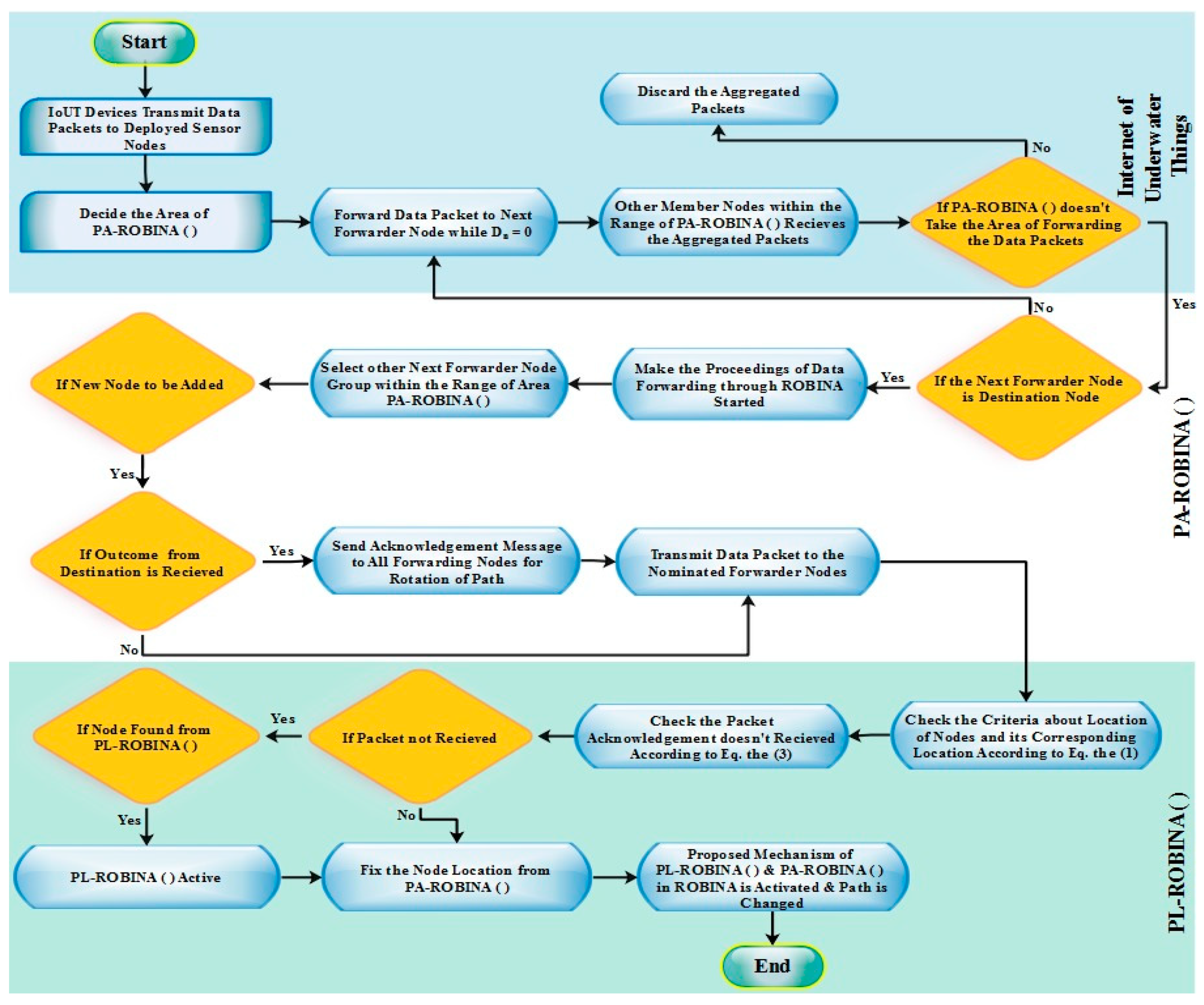
Algorithm 2: Data Delivery Using PA-ROBINA.
  B: Beacon message having next node
  Dn: Number of Dead Nodes
  Sn: Set of Nodes
  Ns: Set of Neighboring nodes
  Adj Ni: Adjacent Nodes
Procedure Area of Path Adjustment (A)
IF |Dn| = 0 then
  Forward data packets ()
  Else
   Dn  takes the next forwarder node (n)
    If |Dn| = 0 then
      for A (AdjNi) = Ns − Dn do
      Forward data S
    Else
      Re-schedule of next forwarder node
      Proposed_scheme ()
    end if
       end for
End IF
  End Procedure

6. Path Loss Channel Model

Rotational Orbit-Based Inter-Node Adjustment (ROBINA) and its Co-variant Path-Adjustment (PA-ROBINA) work for Path-Loss (PL-ROBINA) respectively. Underwater, the acoustic channels are determined by the operating frequency as well as the distance. Here, the operating frequency is only considered between receiver and transmitter as mentioned in [31,32,33]. Underwater path loss dependability is quite different in practice in Terrestrial Wireless Sensor Networks (TWSNs). Path Loss (PL) is determined only by the distance between communication nodes in Radio Frequency (RF) [34] between two communication nodes; particularly, the acoustic signal undergoes a frequency ‘offshore for a distance ‘l’. From the Urick’s Model enlisted in [34], the overall PL is denoted by ‘A(l,f)’; finally, we have to modify it according to the scenario.
A ( l , f ) = l j ( l ( f ) ) d 1000
The ‘j’ represents the circulating factor and describes acoustic signal propagation geometry. Typically, the practical value for ‘K’ in the literature is 1.5. The acoustic pressure into heat for the absorption loss factor α ( f ) is modeled in Equation (4).
According to Thorp’s formula [35], usually ‘f’ measured is KHz as following in Equation (5):
A ( f ) = 10 log ( α ( f ) )   dB / km = 0.11 f 2 1 + f 2 + 40 f 2 4100 + f 2 + 2.75 × 10 4 f 2 + 0.003  
According to [36], there are some main backers defined to the ambient noise like thermal noise Nth (f), turbulence Nth (t), shipping and human activities Ns (f), and wind-driven wave Nw (f), respectively. The continuous Power Spectral Density (PSD) and Colored Gaussian Statistics (CGS) are the major supportive parameters for modeling these equations. Furthermore, the PSD formulae of all these four types of noises with taking frequency ‘f’ (measured in kHz) are given empirically below in Equation (6):
10 log ( N t ( f ) ) = 19 40 log ( f ) 10 log ( N s ( f ) ) = 50 + 30 ( s 0.6 ) + 28 log ( f ) 80 log ( f + 0.04 ) 10 log ( N w ( f ) ) = 60 + 7.5 w 1 2 + 30 log ( f ) 50 log ( f + 0.5 ) 10 log ( N t h ( f ) ) = 18 + 30 log ( f )
Wheres ∈ [0, 1] is defined as 0 in legal shipping activity, ‘f’ in high-level shipment movement, and ‘w’ is the storm velocity measure in m/s; the ‘w’ is also utilized by wind-driven waves that cause surface motion to be captured. Furthermore, the total ambient noise’ N (f)’ is calculated as in Equation (7):
N ( f ) = N t ( f ) + N s ( f ) + N w ( f ) + N t h ( f )
The SNR of an inbound acoustic sound of frequency ‘fi’ transmitted over a distance’ dj, to node ‘n’ is represented as [36].
S N R ( d j , n , f i ) = | a j , n i | 2 P j , n i A ( d j , n , f i ) N ( f i ) B S
where:
(1)
Pij,n shows the power transmission between two nodes.
(2)
N(fi) is the noise power spectral density.
(3)
Bs’ denotes bandwidth on the receiver side.
In multiple scenarios in Underwater, we only assume the fading ratio of a particular channel between two nodes on a limited scale owing to multipath |dij,n|. Here, we assume |aij,n| follows the same work as described in [37,38].
Optimum Acoustic Carrier for Data Transmits Model
The suggested protocol is based on mathematical models that show the smallest amount of transmission that is normally compulsory for data rate per connection. Assume Pij,n is used for transmitting packets from node ‘j’ to node ‘n’ node subcarrier ‘i’. The goal is to determine the lowest feasible transmit power over a set of ‘x’ subcarriers while maintaining the required transmission rate, indicated by ‘R0’ between the nodes ‘j’ and ‘n’. The following is a summary of the entire scenario:
min { i = 1 x P j , n i } ,   s . t . B s i = 1 x log 2 [ 1 + S N R ( d j , n , f i ) ]         R 0   a n d   P j , n i 0     i , j , n
SNR (dj,n, fi) is derived from Equation (8), and ‘x’ is the number of sub-channels utilized by node ‘j’ to send data to node ‘n’. It is worth noting that it is just like the convex function that is used for the objective function.
The function of B s i = 1 x log 2 [ 1 + S N R ( d j , n , f i ) ]   is in terms of Pij. All these details are described in Equation (9) to minimize the cost function [39]. We differentiated Equation (10) with some derivatives by substitution, in which we used ‘ λ ’ as a long-range multiplier.
L { ( P j , n i ) i = 1 x , λ } = i = 1 x P j , n i λ { B s i = 1 x log 2 [ 1 + | a j , n i | 2 P j , n i A ( d j , n , f i ) N ( f i ) B S ] R 0 }
δ L δ P j , n m = 1 λ l n 2 [ | a j , n m | 2 A ( d j , n , f m ) N ( f m ) ] 1 + [ | a j , n m | 2 P j , n m A ( d j , n , f m ) N ( f m ) B S ] = 0  
Here we can elaborate Equation (11) for Pmj,n, as:
1 λ l n 2 [ | a j , n m | 2 A ( d j , n , f m ) N ( f m ) ] = 1 + [ | a j , n m | 2 P j , n m A ( d j , n , f m ) N ( f m ) B S ] l n 2 A ( d j , n , f m ) N ( f m ) λ | a j , n m | 2 l n 2 A ( d j , n , f m ) N ( f m ) = A ( d j , n , f m ) N ( f m ) B S | a j , n m | 2 P j , n m A ( d j , n , f m ) N ( f m ) B S
Since in cross multiplication ‘ P j , n m ’ will disappear and become a free variable, and we can assign any value to it.
B S [ l n 2 A ( d j , n , f m ) N ( f m ) λ | a j , n m | 2 ] = l n 2   [ A ( d j , n , f m ) N ( f m ) B S P j , n m ] P j , n m = B S [ λ | a j , n m | 2 l n 2 A ( d j , n , f m ) N ( f m ) l n 2 | a j , n m | 2
We obtain:
P j , n m = B s [ λ l n 2 A ( d j , n , f m ) N ( f m ) | a j , n m | 2 ] + ,     m = 1 , 2 , , x  
where ‘+’ means to have a source of projections taking non-negative numbers.
δ L δ λ = 0     B s i = 1 x log 2 [ 1 + | a j , n i | 2 P j , n i A ( d j , n , f i ) N ( f i ) B S ] = R 0
We obtain from Equation (14), borrow the Equation (15) values, and perform simple procedures.
λ = [ p a r t 1 p a r t 2 ] ( l n 2 ) ;   w h e r e   p a r t 1 = 2 R 0 x B s   a n d   p a r t 2 = [ i = 1 x | a j , n i | 2 A ( d j , n , f i ) N ( f i ) ] 1 / x
Solving for the minimum power P j , n m we obtain: P j , n m = B S ( p a r t 1 p a r t 2 p a r t 3 p a r t 4 ) + ; where  p a r t 3 = A ( d j , n , f m ) N ( f m )  and  p a r t 4 = | a j , n i | 2 .
Therefore, the number of sub-channel ‘x’ is used by node ‘j’ to transmit data to node ‘n’.

7. Simulation Parameters

The extensive experimental setup connected 700 nodes that start from 50 until it reached its limits, i.e., 700 nodes. A 3D environment with 1600 × 1000 × 1000 dimensional area was used with acoustic link 1500 m/s and 2 kh bandwidth. The Beacon Message size was around 52 bits. All the other parameters like packet size data rates, transmission range, and initial energy were the same as mentioned in [11] and are listed in Table 1. Usually, vertical movement of nodes is not considered underwater; additionally, 2 m/s of horizontal movement was taken into account. Networks simulated NS-2 with version 2.35, along with a dedicated AquaSim framework used for simulations. Table 2 shows the list of simulation values.

7.1. Performing Assessment

In this section, we evaluate the performance of ROBINA against different state-of-the-art routing protocols like EBER2 [14], AEDG [13], ASEDG [11], WDFAD-DBR [15], AVH-AHH-VBF [9], and TANVEER [22]. The parameters were average end-to-end delay, network lifetime, total energy consumption, and packet success ratio. Finally, the overall performance trade-offs of under-observed and some general algorithms in this domain are listed in Table 3.

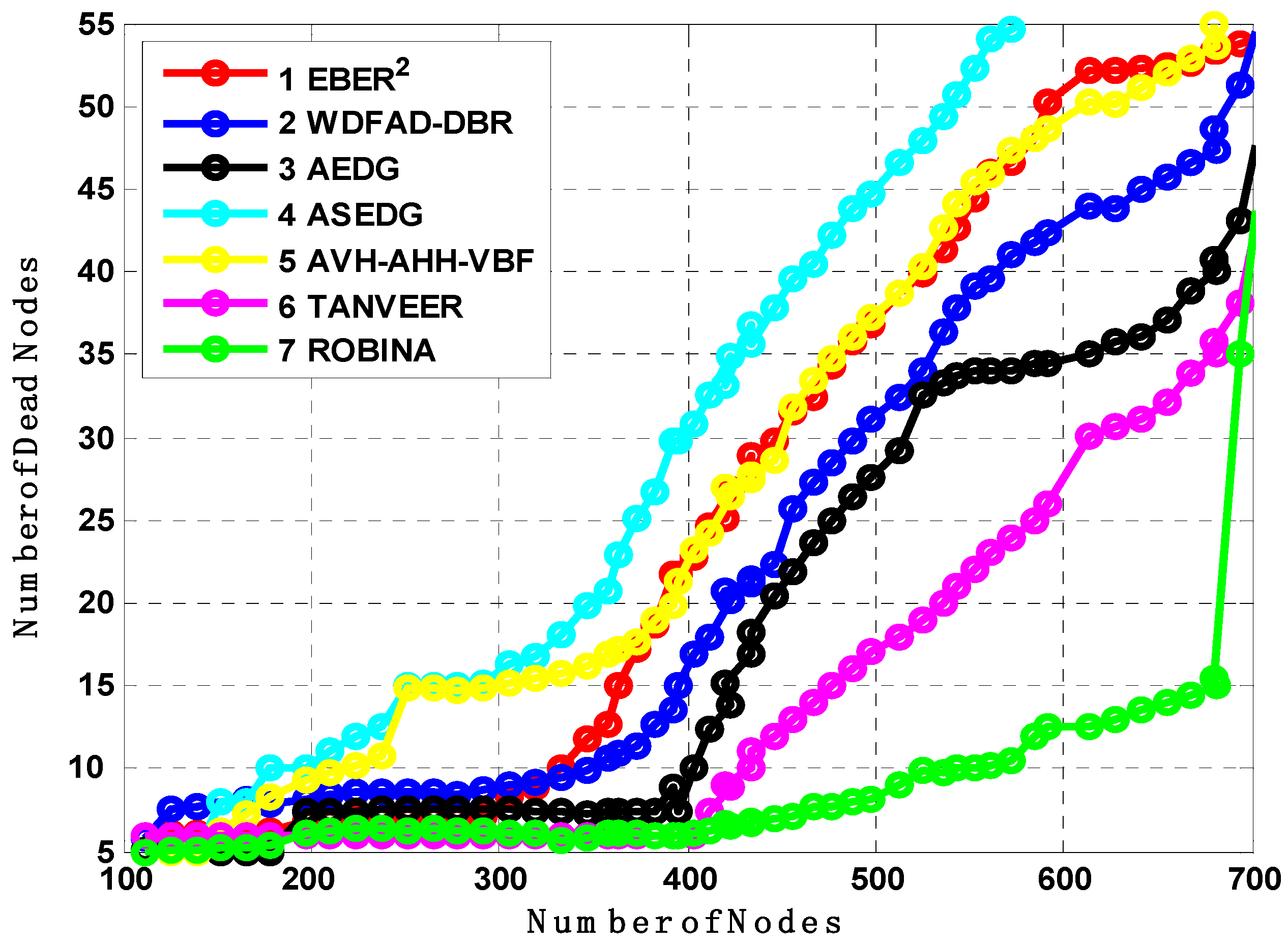
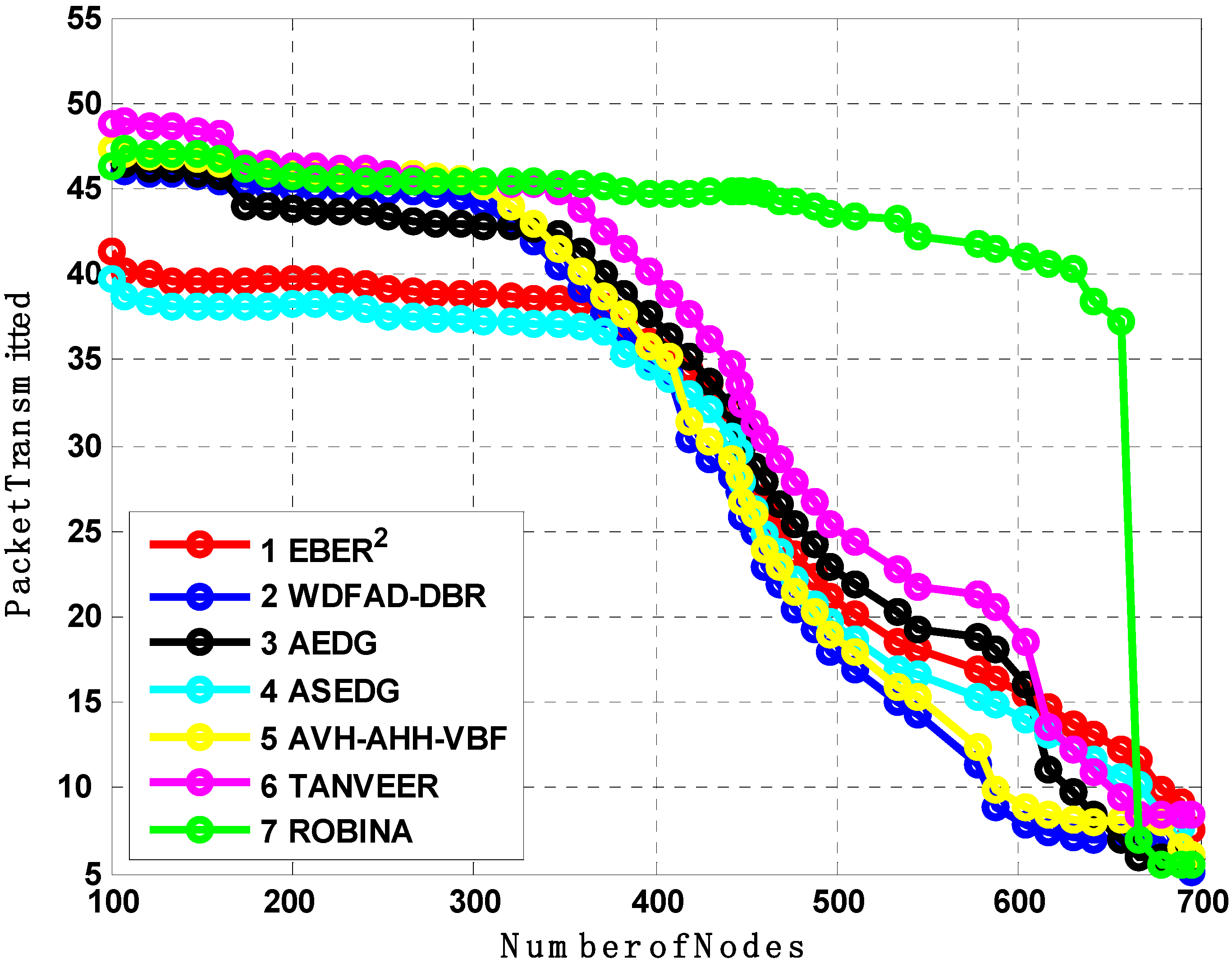
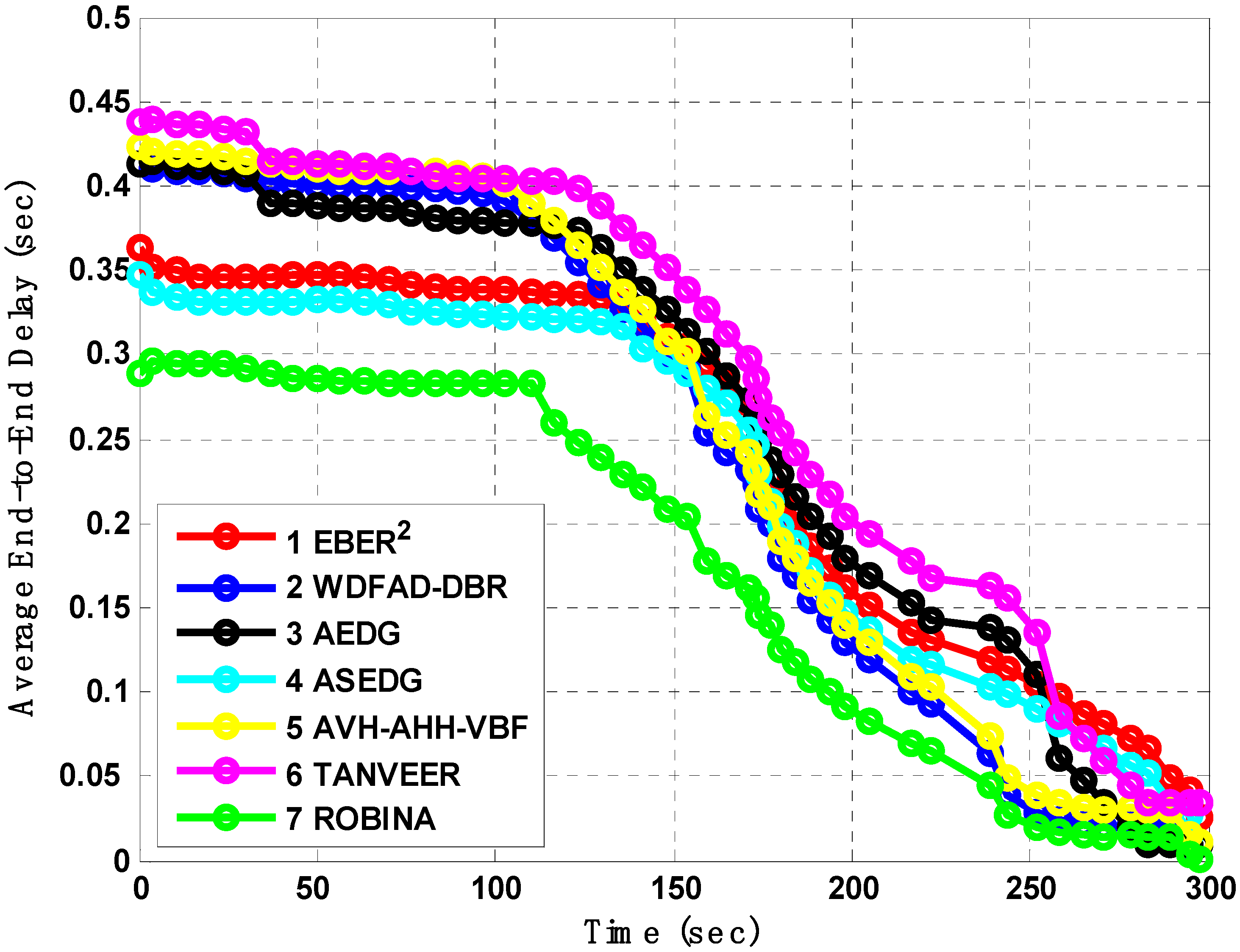
7.2. Analysis of Number of Dead Nodes, Packet Transmitted, and Average End to End Delays

Figure 7, Figure 8 and Figure 9 evaluate all benchmark schemes against the proposed scheme ROBINA. For example, EBER2 is a crook with balance energy and the number of PFN divided among the power level to enhance energy effectiveness. The criteria by which EBER2 selects and deploys PFN is not energy efficient; this is why a large number of nodes (when it is experimental with ROBINA) is nearly boosted up when only the number of nodes is around 400. As the number of nodes increased by 450, it continuously followed the same behavior towards an increasing peak. The same trend is followed by WBFAD-DBR, which chooses the depth of the next forwarder node to avoid void holes. Since mobility is used with AVH-AHH-VBFA, it successfully raises the lifespan of the network with maximum throughput. Therefore, this study showed an outperformance of EBER2 and WDFAD-DBR, respectively when compared with ROBINA as the baseline scheme. It was discovered that AVH-AHH-VBF (due to sinking mobility), WDFAD-DBR (due to using depth divisions with traditional DBR), and EBER2 (due to using (PFN) in its nodes criteria selection) all disregard the following things. (i) criteria towards adjustment of inter-nodes (by any means, either in depth-divisions or PFN and next forwarder nodes). (ii) Selection of shortest path (mentioned in EBER2 and WDFAD-DBR and the hop-base path followed by AVH-AHH-AVBF) instead of the reliable connected path between nodes. (iii) Proof of work (by some mathematical analysis, formula, or some linear equations) is not followed by any existing state-of-the-art schemes. (iv) The path adjustment and path loss (if any) between two connected nodes are not discussed; likewise, all these parameters are covered with PA-ROBINA and PL-ROBINA. Therefore, the total number of dead nodes for EBER2, AVH-AHH-VBF, and WDFAD-DBR are 53, 50, and 52, respectively, when the total number of nodes is experimented in network 700. On the contrary, both AEDG and ASEDG have established the atomic-based path that rotates around the sink and an efficient delay and data-gathering approach that is further divided into atomic-shaped trajectory elliptical for autonomous underwater vehicles (AUVs). Although the path is atomic-shaped and has an elliptical fashion, it is not rotatable. A rotation is missing in AEDG and ASEDG; therefore, most of the relay nodes are not considered, and this is why it is only for 45 nodes against ten iterations, which is comparatively less, and against EBER2, AVH-AHH-VBF, and WDFAD-DBR, respectively, but much higher than ROBINA, which has only 39 dead nodes. TANVEER and ROBINA both show the most interesting results regarding dead nodes. As TANVEER and ROBINA are working to avoid void nodes, even their sub-variants are also working to support the main mechanism. Due to its triangular approach, TANVEER is partially rotated, and ROBINA is a fully rotated orbit-based approach up to 400 nodes; both have the same fashion loss of any nodes as dead. The increasing trend seems to be followed by TANVEER due to its angle cone; as data is forwarding repeatedly and measuring its cone, the rest of the nodes are compiled with energy drastically. Consequently, we can say that as a greater number of nodes appear as dead nodes, ultimately, the performance of packet transmission decreases. Simultaneously, across the board, EBER2, ASEDG, and ASEDG have the same packet transmission ratio, approximately which is 40%. Other schemes, including ROBINA, TANVEER, AEDG, WDFAD-DBR, and AVH-AHH-VBF, have 42%, 43%, 41%, 40%, and 42%, respectively. Among all, ROBINA outperformed and has trade-offs compared with TANVEER, as shown in Figure 8 and Figure 9.

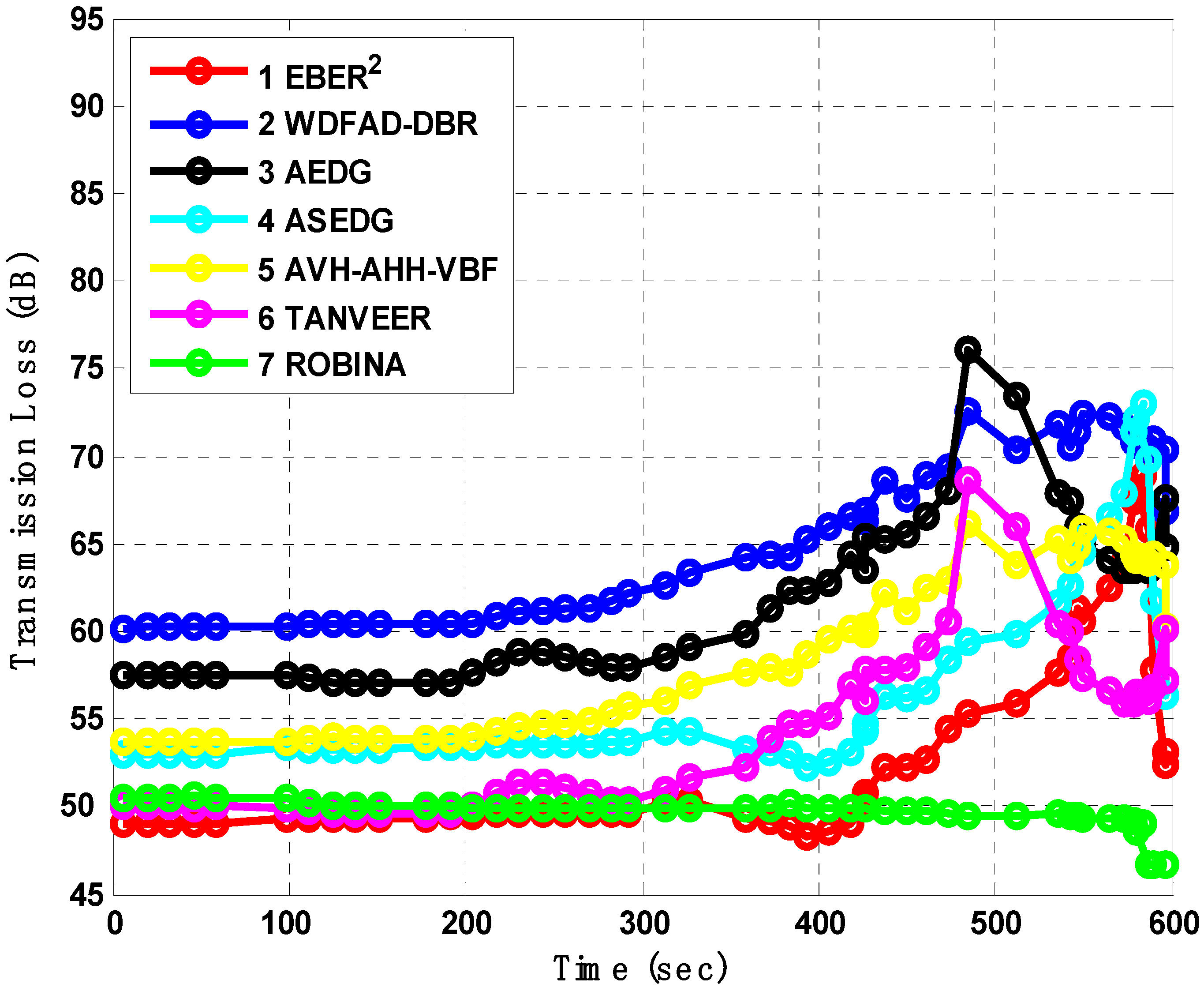
7.3. Analysis of Transmission Loss

We also analyzed the mechanism of transmission loss (which is measured in dB) for intervals of 100 records iteratively, as shown in Figure 10. It is defined as the accumulated decrease in intensity of some network’s behavior to propagate through a certain area. This terminology is frequently used in acoustic scenarios. The following reasons are precuts for this, like the inadequate size of sensors, insulative of distributed sonobuoy low-power factors and weak acoustic links, (which are just mutual like systems that describe the acoustic performance because of large transmission loss underwater), including geometric spreading and sound absorption. Transmission Loss (TL) is a spatial-temporal variable in underwater acoustic channels; thus, it was measured for ROBINA to cross-check the performance of the proposed technique in large deep or shallow water. Ultimately, the TL was comparatively high in all similar schemes, at 50 dB for EBER2 and 50 dB for TANVEER. Both fired next forwarder nodes and Immediate Available Forwarder Nodes (IAFN) during packet transmission; TL was recorded for IAFN (which is used by ROBINA) as approximately 49 dB, which outperformed all benchmark schemes. The minor differences observed in AEDG and ASEDG are due to the Ram nature of underline schemes. For AEDG, the sudden difference is out from 400 to 600 records and increased 55 to 75 dB due to delay and data from schemes. Although a great data gathering scheme, using AUV underwater, taking data from nodes and sending them to sink, is a lengthy process for AEDG and ASEDG. Additionally, WDFAD-DBR and AVH-AHH-VBF had values of 60 dB and 58 dB TL for 500 s until it reached 600.

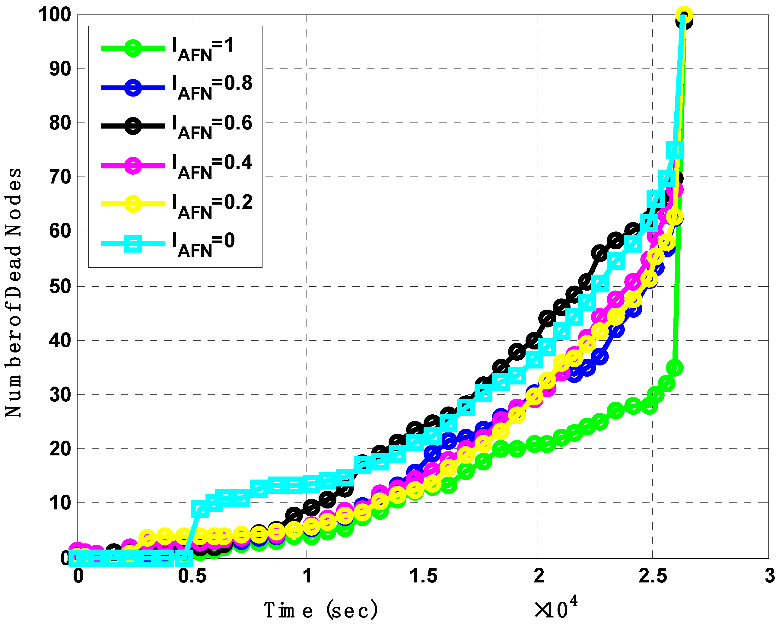
7.4. Impact of Immediate Available Forward Nodes (IAFN)

In our proposed schemes, we also analyzed the effect of the involved parameter of IAFN, which is based upon Algorithms 1 and 2 for ROBINA. The domain and range of this factor are taken from 0 to 1 with equal even intervals. To evaluate the performance of the IAFN, roughly 100 nodes were taken with 0 to 3 recode, though these are recorded for ten thousand. The proper scheme behaved equally when the number of IAFN was between 0.6 to 0.8. For IAFN, at around 2.5 s the total was 38 number of dead nodes of ROBINA. Alternatively, the number of dead nodes increased with IAFN. Usually, the supportive factor in EBER2 is PFN, in AHH-AUV-VBR is VBF, and in WDFAD-DBR is DA division at the role of Member Nodes (MNs) in AEDG and ASEDG, respectively. Like TANVEER, the angled cone and Binary Inter Node (BIN-TANVEER) as supporting roles to map the relay nodes do not go to dead nodes. Therefore, it is closer to our proposed scheme. The following detachment of individual parameters with different periods is shown in Figure 11.

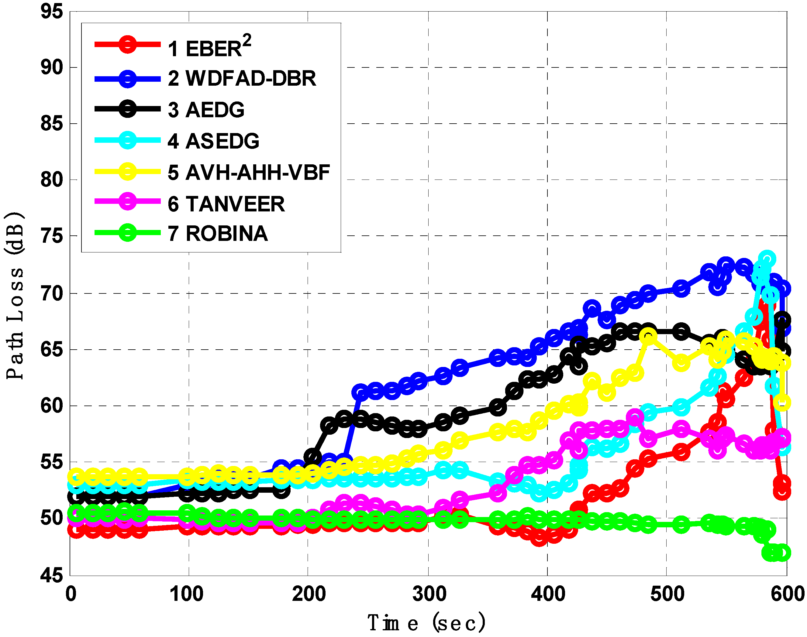
7.5. Analysis of Path Loss

The connection between the two nodes is established when the path remains active; especially in IoUTs, this is a vital concern when the node deploys in a dense environment. Usually, in these types of environments, nodes are particularly far apart from each other and not an intimation of path link breakage. These links suddenly create a void hole for a long time as holes become a void region that isolates the network. Due to the abovementioned reasons, the path analysis between all schemes was experimented and is shown in Figure 12. The WDFAD-DBR and AVH-AHH VBF tackled the depth and coped early to handle the harsh environment; therefore, their path loss was not much increased, only 50 dB and 52 dB, respectively. Rest schemes like EBER2, AEDG, and ASEDG lack such alternatives and, therefore, their path loss analysis satisfied 46 dB, 52 dB, and 53 dB, respectively. The TANVEER and ROBINA had path loss analysis around 200 s equally until it reached 400 s, at which point it increased to 50 dB and 51 dB, respectively. The 1 dB difference is ignorable after 5.5 min of simulation, by principle. Usually, this interval is considered good for out-breaking the result, especially when the critical parameter is under study. On the contrary, ROBINA started at 50 dB and reached the lowest path loss value even after 10 min equal to 600 s.

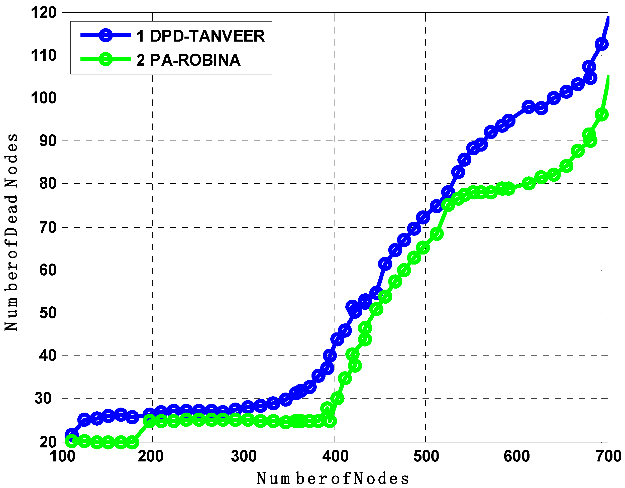
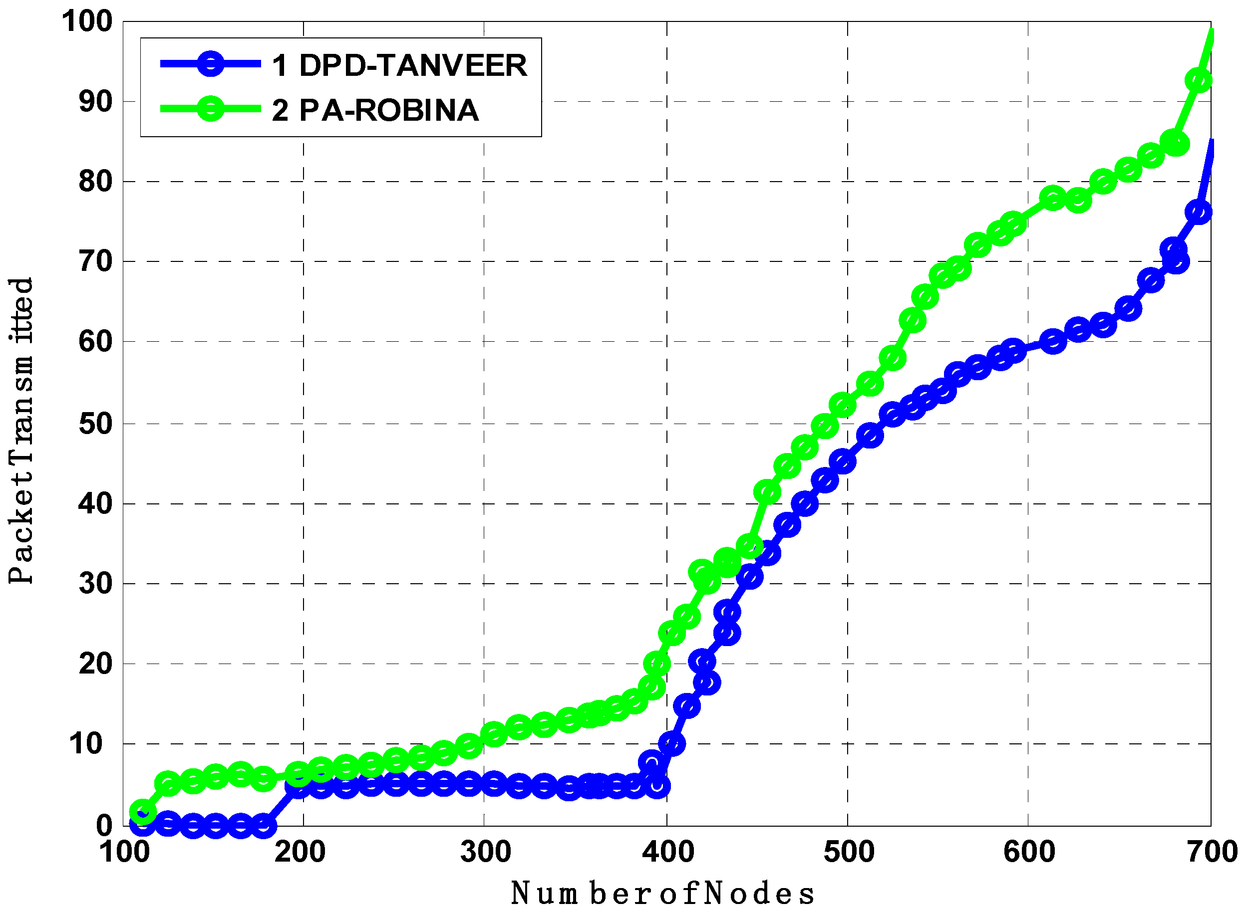
7.6. Analysis of DPD-TANVEER and PA-ROBINA with Number of Dead Nodes and Packet Transmitted

It is evident from Figure 13 that the comparison between DPD-TANVEER (which is a sub-variant of TANVEER for delivery of data Packet, see [22]) and the sub-variant of our proposed approach PA-ROBINA (which is used for enhancing the node length to cover the maximum of relay nodes and IAFN) is represented. With time intervals, the performance of the network including the number of dead nodes was plotting. Initially, the benchmark approach of DPD-TANVEER had a smaller number of dead nodes until the first 50 s to 100 s, and the total number of dead nodes found less than one were ignorable. Suddenly, the next interval of 50 s, like in 150 s until it reaches 250 s, the number of nodes increased, which was eight nodes for PA-ROBINA and around ten nodes for DPD-TANVEER. During path adjustment, most of the nodes are easily covered under the radius of the destination.
Furthermore, the PA-ROBINA also considered forwarder nodes distances; therefore, the closer nodes were easily covered. Meanwhile, in DPD-TANVEER, the speed purpose nodes are called watchman nodes, responsible for providing the immediate alternate rotation for dead nodes. As watchman nodes use some amount of energy, the time to recover and rescue the dead nodes is longer than ROBINA. As the number of dead nodes is decreased, the packed transmission is increased. It is earlier mentioned that the procedure of both TANVEER and ROBINA techniques, therefore, consider and analyze the effect of Figure 13 on Figure 14. Although, the packet transmission of PA-ROBINA is majorly increased and dominant over DPD-TANVEER.

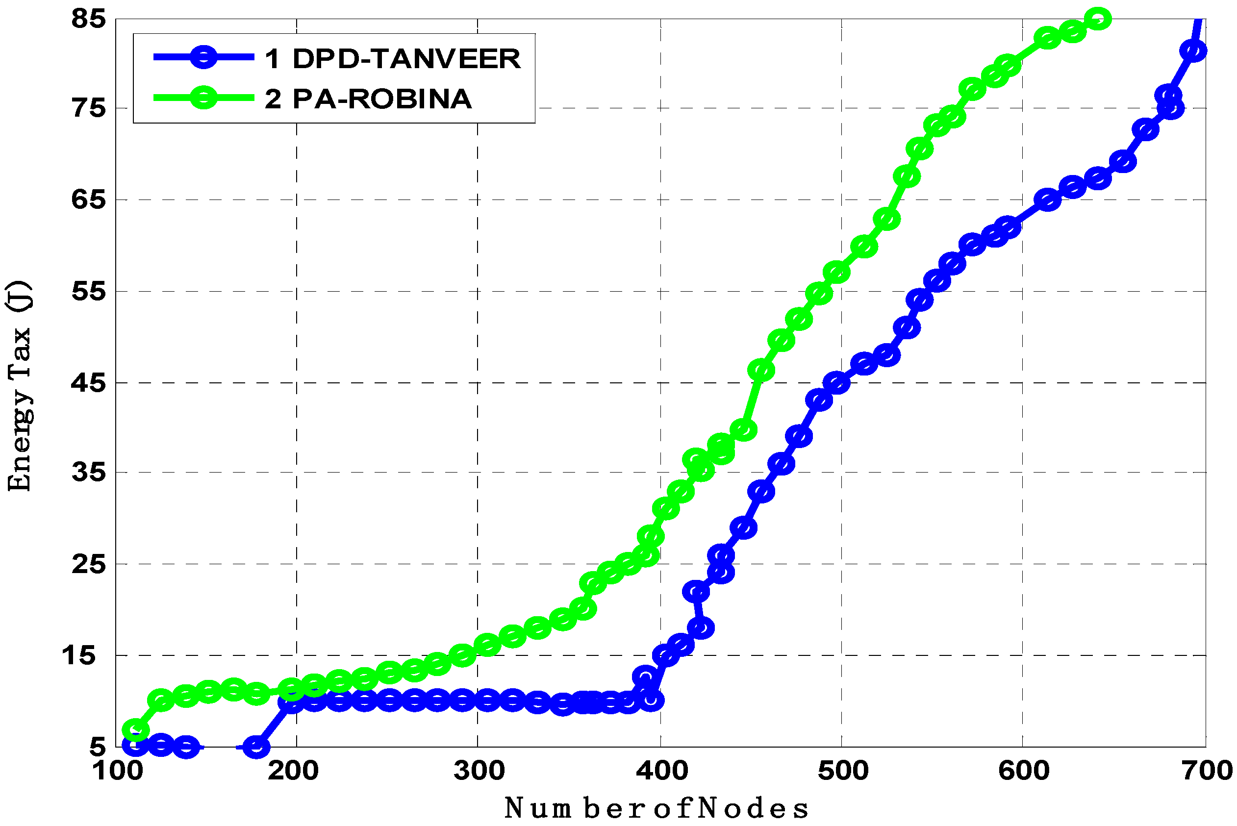
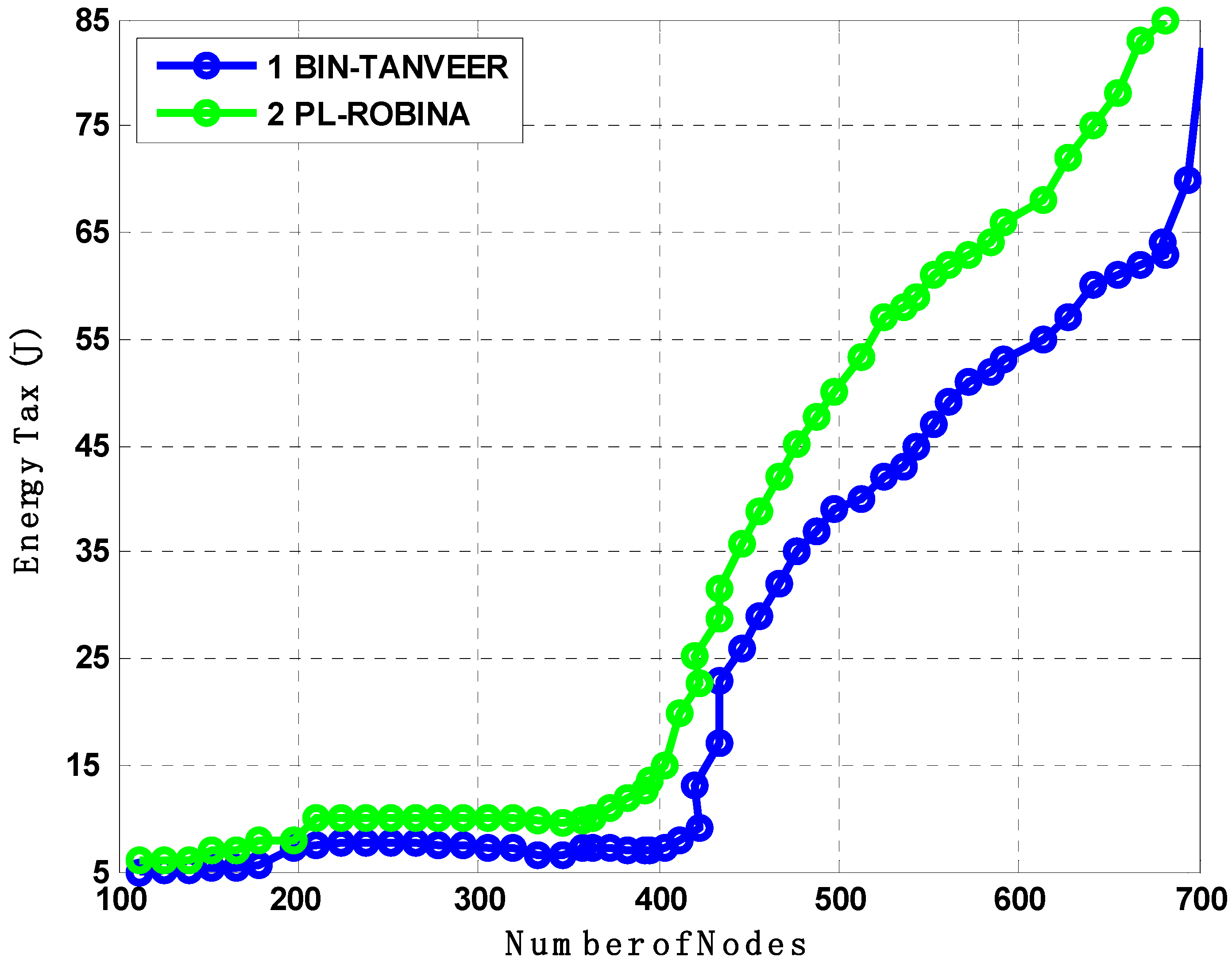
7.7. Analysis of DPD-TANVEER and PA-ROBINA with Energy Tax

The amount of EC was experimented with and shown in Figure 15 between ROBINA with its other selected similar state-of-the-art schemes. Energy is the fundamental parameter in all routing protocols, even where the unmanned efforts requiring the replacements of nodes or batteries are much more difficult. Due to the atomic path with its MNs used in AEDG and ASEDG, EC is higher than WDFAD-DBR and EBER2, which we did not consider in experiments because ROBINA used the capacity of internodes adjustment and had a mechanism to avoid void holes. Hence, it saved the most energy among all routing schemes when it was used.
Energy is the primary restriction in all routing strategies regardless of the strategy or technique employed. As a result, Figure 15 compares the energy usage of DPD-TANVEER and PA-ROBINA. During the transfer of packets from source to destination, energy tax analyses were performed. When the network was not dense, the tax was not eaten as much as in DPD-TANVEER; because TANVEER skips the empty areas and sends the data packet directly to the runabout, it is slightly slower than PA-ROBINA. With DPD-TANVEER, the least potential energy consumption was counted at 0.6 J for 150 nodes and 0.8 J when nodes approached their limit. This is due to triangle-baud measurement when the angled cone is determined for the data packet’s destination through all directions. It is interesting to note that the DPD-TANVEER was comparatively high when simulated with L2-ABF, though still somewhat lower (i.e., slightly lower) when compared to PA-ROBINA. The adjustment and consumption method for relay nodes and (IAFN) was slightly better than its data delivery; because of the large-scale network (we employed 800 nodes in ROBINA and 200 nodes in TANVEER), the IoUTs are frequently unpredictable, especially regarding energy tax. The cost of node mobility in this scenario is not a positive factor, and the amount of energy is purposely loaded. Meanwhile, the ROBINA outperformed in these scenarios and covered both (water/node movement, frequently charged topology, dynamic and static sinks stations, acute communication, and water current, which is also unpredictable with dense to shallow water) using the rotation-based path and mechanism of inter-node adjustment. When a medium to the large-scale network was eliminated as a text-bed, the amount indicated by our technique was not debatable; [34,35,36,37,38,39] is a good example for this understanding.

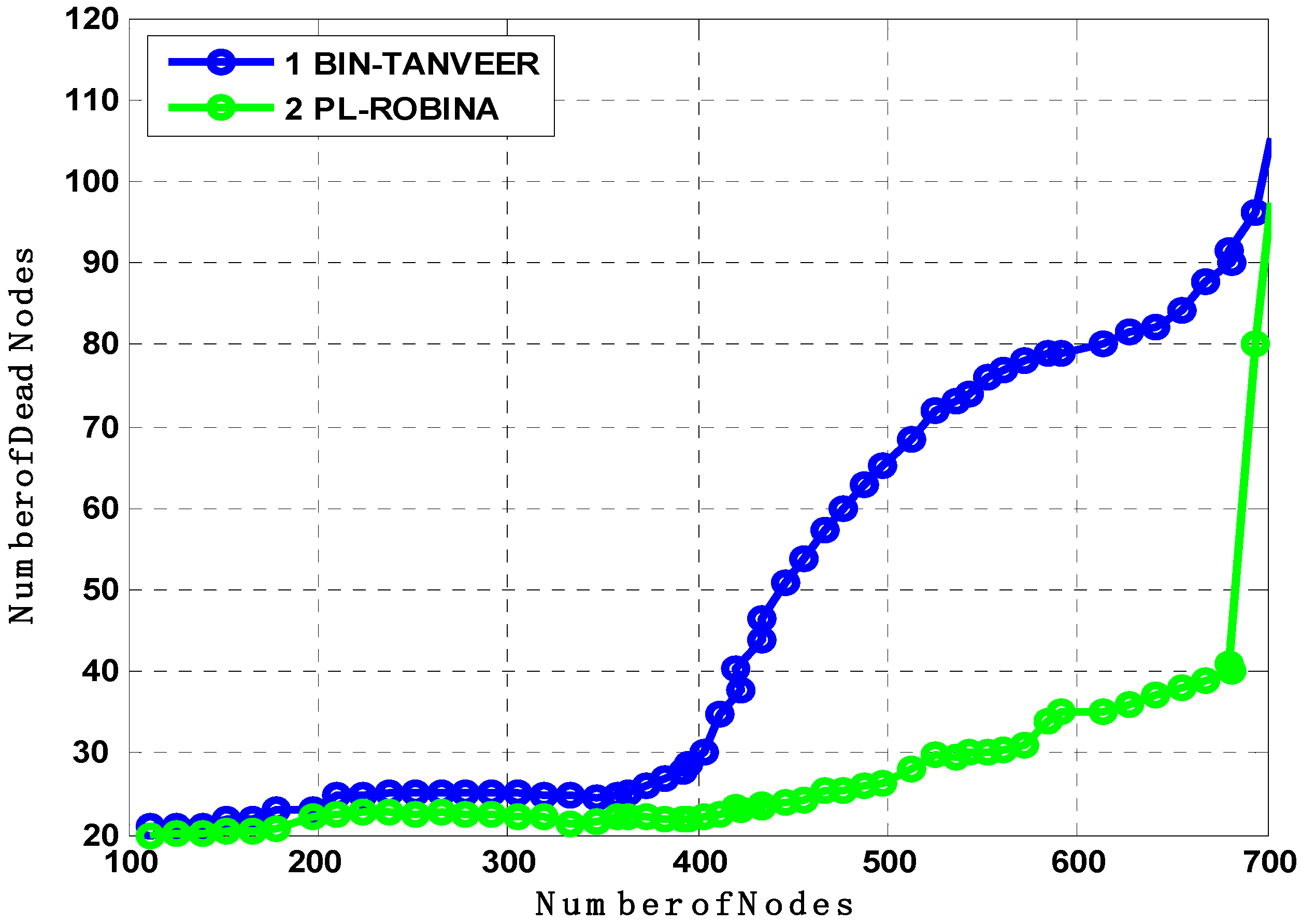
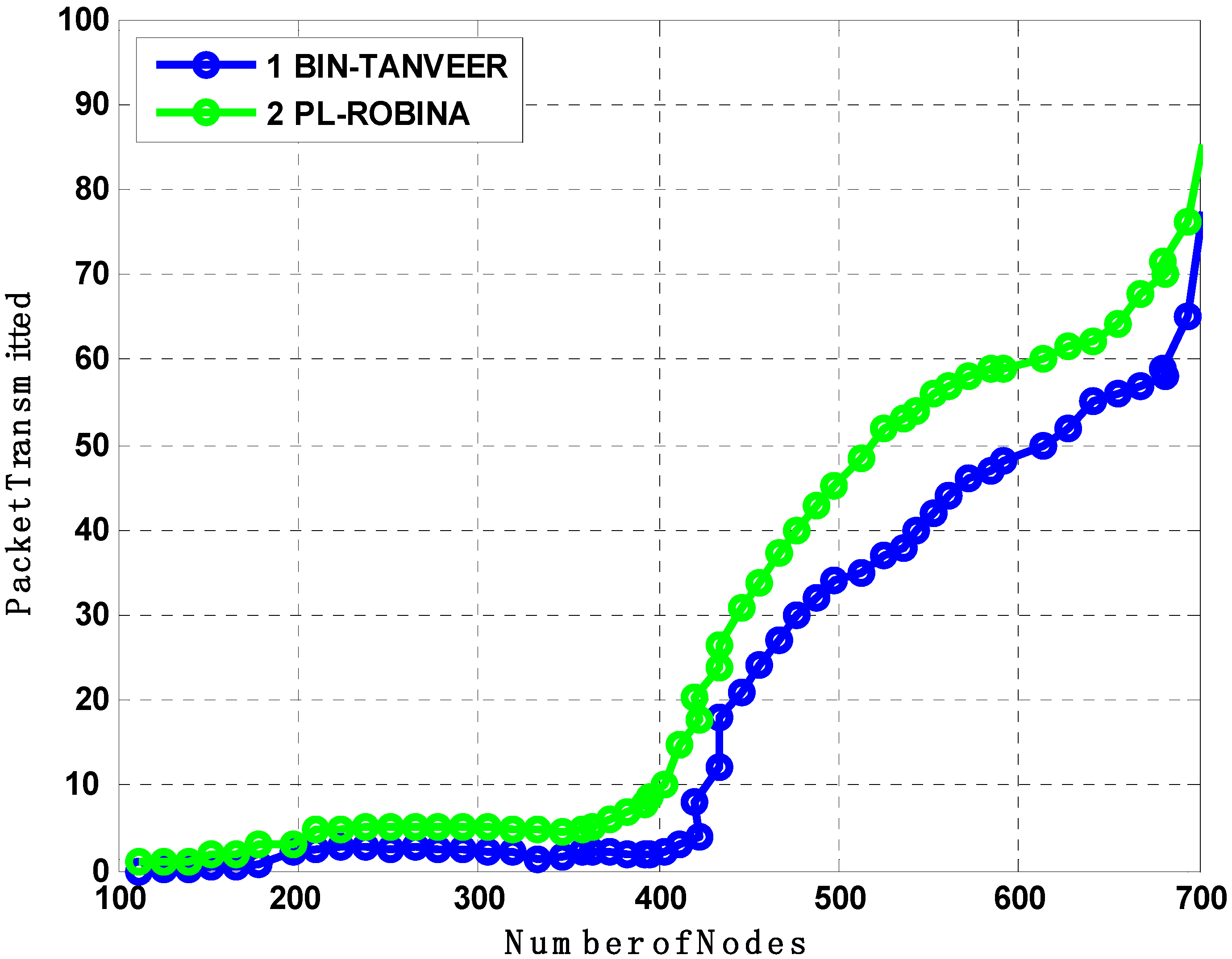
7.8. Analysis of BIN-TANVEER and PL-ROBINA with Number of Dead Nodes and Packet Transmitted

The BIN-TANVEER and PL-ROBINA relation is presented the same scenario of finding the number of dead nodes in Figure 16. The path-loss mechanism is supported by Uricks model and the Colored Gaussians Surface (CGS) for optimizing the routing path and acute signal between two communicated nodes, so the path loss is dubbed according to Equation (1). Typically, with the use of the practical value of ‘K’ with ‘Throps formula’ for derivative by integration, it has been observed that the existing monitoring IoT system with some routing mechanism ignores the factor of path loss (here, we considered the path loss between only two communicated IoT devices (whatever the way underwater) and the main concern was its recovery as well as detection to find out the health of the network when the path was not found, for the time being, between two devices) to ensure if it recovers from two connected devices and if recovery is so for all devices (connected) in the routing path by the help of ‘Tylor and Maclaren Series’ that already used in sensor data cryptography [40,41,42]. Therefore, the path loss is best described in the PL-ROBINA scheme over BIN-TANVEER. Although the PL-ROBINA outperformed even the largest number of nodes (say 750 from Figure 16), the BIN-TANVEER has only handled the nodes and their dead quantity with suitable energy tax when the network was in the category of the small to medium scale, as contrary to PL-ROBINA for medium to large-scale networks. Ultimately, the packet transmission is also attached as for the energy tax from Figure 17 and Figure 18. From Figure 17, the performance of PL-ROBINA is satisfactory as evidenced by its large number of packets transmitted due to the non-loss of the path between two connected devices; BIN-TANVEER cannot handle a large amount of data, as the Binary Inter Nodes (BIN’s) are not functional enough and supported with this kind of situation. It is only built on purpose in TANVEER, and as mentioned in [22], the packet success ratio achieved 94% of ROBINA and AVH-AHH-VBF. In addition, the WDFAD-DBR has the least ratio, which is only 62%. Meanwhile, the same situation will be observed for energy tax with BIN-TANVEER and PL-ROBINA respectively.

8. Conclusions

The void hole problem has a long-lasting effect in the acoustic environment that attracts lots of attention from the research community. In order to address this problem for the sake of performance analysis and evaluation, we performed extensive simulation against the different number of dead nodes: packet transmission, energy tax, transmission loss, and path loss mechanism with state-of-the-art techniques like EBER2, AEDG, ASEDG, WDFAD-DBR, AVH-AHH-VBF, and TANVEER. Simulated results showed that our proposed scheme performed better to increase high packet transmission and minimum transmission loss and path loss with affordable E2E delays. Therefore, we offered a novel avenue that has rotational orbits based on its mechanism of inter-node adjustment that has affordable E2E, which is 0.2 and remains constant. The EC and network lifetime also had good simulation results due to their path adjustment (that had orbital shapes) mechanisms. We also improved the packet transmission through this scheme around 68–92%, even in a dense network. Comparatively, all other schemes were not yet experimental when the network was dense (say 500 number of the node). Overall, we can conclude that the ROBINA outperformed against EBER2 and WDFAD-DBR in terms of E2E and transmission loss, which was 60% higher than the abovementioned. Moreover, the AEDG and ASEDG were experimental against packet success ratio and path loss the proposed scheme, ROBINA, have similar results due to the dense avoidance of void hole problems compared with TANVEER and its variants. In the future, we have the intention to simulate ROBINA and propose a similar technique that enables blockchain technology for very large-scale networks with a testbed, large oceanic environment.

Author Contributions

U.D. and S.Y. proposed the research conceptualization and methodology. The technical and theoretical framework was prepared by S.Y., T.A. and A.A. The technical review and improvement were performed by A.A. and T.A., N.Z. and D.-Y.S. performed the overall technical support, guidance, and project administration. The editing and, finally, proofreading was performed M.H.J. and Z.B.F. All authors have read and agreed to the published version of the manuscript.

Funding

This research was supported by the MSIT(Ministry of Science and ICT), Korea, under the Grand Information Technology Research Center support program(IITP-2021-2015-0-00742) supervised by the IITP(Institute for Information & communications Technology Planning & Evaluation).

Institutional Review Board Statement

Not applicable.

Informed Consent Statement

Not applicable.

Data Availability Statement

Not applicable.

Acknowledgments

The authors acknowledge the support from the University of Sahiwal, University of Okara, and COMSATS University Islamabad, Including Lahore and Sahiwal Campus. As the principal author, I would like to say especially vote of thanks to my ample co-author Sana Yasin and her speechless idea support to accomplish my dream project on time. The true mirror support of Tariq Ali, Amjad Ali and Ning Zhang; those persons who support me in every technical step without any hesitation are appreciated.

Conflicts of Interest

The authors declare that there is no conflict of interest.

References

  1. Jamali, M.V.; Chizari, A.; Salehi, J.A. Performance analysis of multi-hop underwater wireless optical communication systems. IEEE Photonics Technol. Lett. 2017, 29, 462–465. [Google Scholar] [CrossRef]
  2. Boucouvalas, A.C.; Peppas, K.P.; Yiannopoulos, K.; Ghassemlooy, Z. Underwater optical wireless communications with optical amplification and spatial diversity. IEEE Photonics Technol. Lett. 2016, 28, 2613–2616. [Google Scholar] [CrossRef]
  3. Xiao, L.; Sheng, G.; Wan, X.; Su, W.; Cheng, P. Learning-based PHY-layer authentication for underwater sensor networks. IEEE Commun. Lett. 2018, 23, 60–63. [Google Scholar] [CrossRef]
  4. Yan, J.; Tian, X.; Luo, X.; Guan, X. Design of an Embedded Communication System for Underwater Asynchronous Localization. IEEE Embed. Syst. Lett. 2019, 11, 97–100. [Google Scholar] [CrossRef]
  5. Zhao, R.; Li, N.; Dobre, O.A.; Shen, X. CITP: Collision and Interruption Tolerant Protocol for Underwater Acoustic Sensor Networks. IEEE Commun. Lett. 2020, 24, 1328–1332. [Google Scholar] [CrossRef]
  6. Li, S.; Qu, W.; Liu, C.; Qiu, T.; Zhao, Z. Survey on high reliability wireless communication for underwater sensor networks. J. Netw. Comput. Appl. 2019, 148, 102446. [Google Scholar] [CrossRef]
  7. John, S.; Menon, V.G.; Nayyar, A. Simulation-Based Performance Analysis of Location-Based Opportunistic Routing Protocols in Underwater Sensor Networks Having Communication Voids. In Data Management, Analytics and Innovation; Springer: Singapore, 2020; pp. 697–711. [Google Scholar]
  8. Latif, K.; Javaid, N.; Ullah, I.; Kaleem, Z.; Abbas, Z.; Nguyen, L.D. DIEER: Delay-Intolerant Energy-Efficient Routing with Sink Mobility in Underwater Wireless Sensor Networks. Sensors 2020, 20, 3467. [Google Scholar] [CrossRef] [PubMed]
  9. Hussain, T.; Rehman, Z.U.; Iqbal, A.; Saeed, K.; Ali, I. Two hop verification for avoiding void hole in underwater wireless sensor network using SM-AHH-VBF and AVH-AHH-VBF routing protocols. Trans. Emerg. Telecommun. Technol. 2020, 31, e3992. [Google Scholar] [CrossRef]
  10. Wadud, Z.; Ismail, M.; Qazi, A.B.; Khan, F.A.; Derhab, A.; Ahmad, I.; Ahmad, A.M. An Energy Balanced Efficient and Reliable Routing Protocol for Underwater Wireless Sensor Networks. IEEE Access 2019, 7, 175980–175999. [Google Scholar] [CrossRef]
  11. Farooq, W.; Ali, T.; Shaf, A.; UMAR, M.; Yasin, S. Atomic-shaped efficient delay and data gathering routing protocol for underwater wireless sensor networks. Turk. J. Electr. Eng. Comput. Sci. 2019, 27, 3454–3469. [Google Scholar] [CrossRef] [Green Version]
  12. Draz, M.U.; Ali, T.; Yasin, S.; Waqas, U. Towards formal modeling of hotspot issue by watch-man nodes in wireless sensor and actor network. In Proceedings of the IEEE 2018 International Conference on Frontiers of Information Technology (FIT), Islamabad, Pakistan, 17–19 December 2018; pp. 321–326. [Google Scholar]
  13. Ilyas, N.; Alghamdi, T.A.; Farooq, M.N.; Mehboob, B.; Sadiq, A.H.; Qasim, U.; Javaid, N. AEDG: AUV-aided Efficient Data Gathering Routing Protocol for Underwater Wireless Sensor Networks. In Proceedings of the ANT/SEIT, London, UK, 2–5 January 2015; pp. 568–575. [Google Scholar]
  14. Wang, H.; Zhang, X.; Khokhar, A. Efficient ”void” handling in contention-based geographic routing for wireless sensor networks. In Proceedings of the IEEE GLOBECOM 2007-IEEE Global Telecommunications Conference 2007, Washington, DC, USA, 26–30 November 2007; pp. 663–667. [Google Scholar]
  15. Yu, H.; Yao, N.; Wang, T.; Li, G.; Gao, Z.; Tan, G. WDFAD-DBR: Weighting depth and forwarding area division DBR routing protocol for UASNs. Ad Hoc Netw. 2016, 37, 256–282. [Google Scholar] [CrossRef]
  16. Ozawa, M. Position measuring interactions and the Heisenberg uncertainty principle. Phys. Lett. A 2002, 299, 1–7. [Google Scholar] [CrossRef] [Green Version]
  17. Derevenskii, V.P. Matrix Bernoulli Equations. I. Russ. Math. 2008, 52, 12–21. [Google Scholar] [CrossRef]
  18. Sher, A.; Khan, A.; Javaid, N.; Ahmed, S.H.; Aalsalem, M.Y.; Khan, W.Z. Void hole avoidance for reliable data delivery in IoT enabled underwater wireless sensor networks. Sensors 2018, 18, 3271. [Google Scholar] [CrossRef] [PubMed] [Green Version]
  19. Ahmed, F.; Gul, S.; Khalil, M.A.; Sher, A.; Khan, Z.A.; Qasim, U.; Javed, N. Two Hop Adaptive Routing Protocol for Underwater Wireless Sensor Networks. In Proceedings of the International Conference on Innovative Mobile and Internet Services in Ubiquitous Computing, Torino, Italy, 10–12 July 2017; Springer: Cham, Switzerland, 2017; pp. 181–189. [Google Scholar]
  20. Zhang, X.M.; Wang, E.B.; Xia, J.J.; Sung, D.K. An estimated distance-based routing protocol for mobile ad hoc networks. IEEE Trans. Veh. Technol. 2011, 60, 3473–3484. [Google Scholar] [CrossRef]
  21. Gopi, S.; Govindan, K.; Chander, D.; Desai, U.B.; Merchant, S.N. E-PULRP: Energy optimized path unaware layered routing protocol for underwater sensor networks. IEEE Trans. Wirel. Commun. 2010, 9, 3391–3401. [Google Scholar] [CrossRef]
  22. Draz, U.; Yasin, S.; Irfan, M.; Ali, T.; Ali, A.; Glowacz, A.; Glowacz, W. TANVEER: Tri-Angular Nearest Vector-Based Energy Efficient Routing for IoT-Enabled Acoustic Sensor and Actor Networks (I-ASANs). Sensors 2021, 21, 3578. [Google Scholar] [CrossRef]
  23. Coutinho, R.W.; Boukerche, A. Stochastic Modeling of Opportunistic Routing in Multi-Modal Internet of Underwater Things. In Proceedings of the GLOBECOM 2020-2020 IEEE Global Communications Conference, Taipei, Taiwan, 7–11 December 2020; pp. 1–6. [Google Scholar]
  24. Chandavarkar, B.R.; Gadagkar, A.V. Expectation-Based Multi-Attribute Multi-Hop Routing (EM 2 R) in Underwater Acoustic Sensor Networks. In Proceedings of the 2020 IEEE 15th International Conference on Industrial and Information Systems (ICIIS), Rupnagar, India, 26–28 November 2020; pp. 555–560. [Google Scholar]
  25. Draz, U.; Ali, T.; Ahmad Zafar, N.; Saeed Alwadie, A.; Irfan, M.; Yasin, S.; Khan Khattak, M.A. Energy efficient watchman-based flooding algorithm for IoT-enabled underwater wireless sensor and actor networks. ETRI J. 2021. Available online: https://onlinelibrary.wiley.com/doi/full/10.4218/etrij.2019-0591 (accessed on 10 July 2021). [CrossRef]
  26. Al-Salti, F.; Alzeidi, N.; Day, K. Localization Schemes for Underwater Wireless Sensor Networks: Survey. Int. J. Comput. Netw. Commun. 2020, 12, 113–130. [Google Scholar] [CrossRef]
  27. Alasarpanahi, H.; Ayatollahitafti, V.; Gandomi, A. Energy-efficient void avoidance geographic routing protocol for underwater sensor networks. Int. J. Commun. Syst. 2020, 33, e4218. [Google Scholar] [CrossRef]
  28. Gola, K.K.; Gupta, B. Underwater acoustic sensor networks: An energy efficient and void avoidance routing based on grey wolf optimization algorithm. Arab. J. Sci. Eng. 2021, 46, 3939–3954. [Google Scholar] [CrossRef]
  29. Draz, U.; Ali, T.; Yasin, S.; Naseer, N.; Waqas, U. A parametric performance evaluation of SMDBRP and AEDGRP routing protocols in underwater wireless sensor network for data transmission. In Proceedings of the IEEE 2018 International Conference on Advancements in Computational Sciences (ICACS), Lahore, Pakistan, 19–21 February 2018; pp. 1–8. [Google Scholar]
  30. Halakarnimath, B.S.; Sutagundar, A.V. Reinforcement Learning-Based Routing in Underwater Acoustic Sensor Networks. Wirel. Pers. Commun. 2021, 120, 419–446. [Google Scholar] [CrossRef]
  31. El-Banna, A.A.A.; Wu, K. Introduction to Underwater Communication and IoUT Networks. In Machine Learning Modeling for IoUT Networks; Springer: Cham, Swirzerland, 2021; pp. 1–8. [Google Scholar]
  32. Ali, T.; Yasin, S.; Draz, U.; Ayaz, M. Towards formal modeling of subnet based hotspot algorithm in wireless sensor networks. Wirel. Pers. Commun. 2019, 107, 1573–1606. [Google Scholar] [CrossRef]
  33. Coutinho, R.W.; Boukerche, A. OMUS: Efficient Opportunistic Routing in Multi-Modal Underwater Sensor Networks. IEEE Trans. Wirel. Commun. 2021. [Google Scholar] [CrossRef]
  34. Jan, S.; Yafi, E.; Hafeez, A.; Khatana, H.W.; Hussain, S.; Akhtar, R.; Wadud, Z. Investigating Master–Slave Architecture for Underwater Wireless Sensor Network. Sensors 2021, 21, 3000. [Google Scholar] [CrossRef]
  35. Nguyen, N.T.; Le, T.T.; Nguyen, H.H.; Voznak, M. Energy-efficient clustering multi-hop routing protocol in a UWSN. Sensors 2021, 21, 627. [Google Scholar] [CrossRef]
  36. Draz, U.; Ali, T.; Yasin, S. Cloud Based Watchman Inlets for Flood Recovery System Using Wireless Sensor and Actor Networks. In Proceedings of the 2018 IEEE 21st International Multi-Topic Conference (INMIC), Karachi, Pakistan, 1–2 November 2018; pp. 1–6. [Google Scholar]
  37. Zhao, D.; Lun, G.; Xue, R.; Sun, Y. Cross-Layer-Aided Opportunistic Routing for Sparse Underwater Wireless Sensor Networks. Sensors 2021, 21, 3205. [Google Scholar] [CrossRef]
  38. Ashraf, S.; Ahmed, T.; Raza, A.; Naeem, H. Design of shrewd underwater routing synergy using porous energy shells. Smart Cities 2020, 3, 74–92. [Google Scholar] [CrossRef] [Green Version]
  39. Draz, U.; Yasin, S.; Ali, A.; Khan, M.A.; Nawaz, A. Traffic Agents-Based Analysis of Hotspot Effect in IoT-Enabled Wireless Sensor Network. In Proceedings of the IEEE 2021 International Bhurban Conference on Applied Sciences and Technologies (IBCAST), Islamabad, Pakistan, 14–18 January 2021; pp. 1029–1034. [Google Scholar]
  40. Luo, J.; Chen, Y.; Wu, M.; Yang, Y. A Survey of Routing Protocols for Underwater Wireless Sensor Networks. IEEE Commun. Surv. Tutor. 2021, 23, 137–160. [Google Scholar] [CrossRef]
  41. Aysal, T.C.; Barner, K.E. Sensor data cryptography in wireless sensor networks. IEEE Trans. Inf. Forensics Secur. 2008, 3, 273–289. [Google Scholar] [CrossRef]
  42. Ortigueira, M.D.; Trujillo, J.J.; Martynyuk, V.I.; Coito, F.J. A generalized power series and its application in the inversion of transfer functions. Signal Process. 2015, 107, 238–245. [Google Scholar] [CrossRef]
  43. Mahmutoglu, Y.; Turk, K.; Tugcu, E. Particle swarm optimization algorithm based decision feedback equalizer for underwater acoustic communication. In Proceedings of the IEEE 2016 39th International Conference on Telecommunications and Signal Processing (TSP), Vienna, Austria, 27–29 June 2016; pp. 153–156. [Google Scholar]
  44. Zhang, J.; Cao, Y.; Han, G.; Fu, X. Deep neural network-based underwater OFDM receiver. IET Commun. 2019, 13, 1998–2002. [Google Scholar] [CrossRef]
  45. Chen, Y.; Yu, W.; Sun, X.; Wan, L.; Tao, Y.; Xu, X. Environment-aware communication channel quality prediction for underwater acoustic transmissions: A machine learning method. Appl. Acoust. 2021, 181, 108128. [Google Scholar] [CrossRef]
  46. Su, Y.; Liwang, M.; Gao, Z.; Huang, L.; Du, X.; Guizani, M. Optimal cooperative relaying and power control for IoUT networks with reinforcement learning. IEEE Internet Things J. 2020, 8, 791–801. [Google Scholar] [CrossRef]
  47. Jin, Z.; Zhao, Q.; Su, Y. RCAR: A reinforcement-learning-based routing protocol for congestion-avoided underwater acoustic sensor networks. IEEE Sens. J. 2019, 19, 10881–10891. [Google Scholar] [CrossRef]
  48. Su, Y.; Fan, R.; Fu, X.; Jin, Z. DQELR: An adaptive deep Q-network-based energy-and latency-aware routing protocol design for underwater acoustic sensor networks. IEEE Access 2019, 7, 9091–9104. [Google Scholar] [CrossRef]
  49. Alamgir, M.S.M.; Sultana, M.N.; Chang, K. Link adaptation on an underwater communications network using machine learning algorithms: Boosted regression tree approach. IEEE Access 2020, 8, 73957–73971. [Google Scholar] [CrossRef]
  50. Pabani, J.K.; Luque-Nieto, M.Á.; Hyder, W.; Otero, P. Energy-Efficient Packet Forwarding Scheme Based on Fuzzy Decision-Making in Underwater Sensor Networks. Sensors 2021, 21, 4368. [Google Scholar] [CrossRef]
  51. Shaf, A.; Ali, T.; Farooq, W.; Draz, U.; Yasin, S. Comparison of DBR and L2-ABF routing protocols in underwater wireless sensor network. In Proceedings of the IEEE 2018 15th International Bhurban Conference on Applied Sciences and Technology (IBCAST), Islamabad, Pakistan, 14–18 January 2018; pp. 746–750. [Google Scholar]
  52. Ali, T.; Ayaz, M.; Jung, L.T.; Draz, U.; Shaf, A. Upward and diagonal data packet forwarding in underwater communication. ESTIRJ 2017, 1, 33–40. [Google Scholar]
  53. Draz, U.; Ali, T.; Asghar, K.; Yasin, S.; Sharif, Z.; Abbas, Q.; Aman, S. A Comprehensive Comparative Analysis of Two Novel Underwater Routing Protocols. IJACSA 2019, 10, 4. [Google Scholar] [CrossRef]
  54. Anum, A.; Ali, T.; Akbar, S.; Obaid, I.; Junaid, M.; Anjum, U.D.; Shaheen, M. Angle Adjustment for Vertical and Diagonal Communication in underwater Sensor Networks. IJACSA Int. J. Adv. Comput. Sci. Appl. 2020, 11, 604–616. [Google Scholar]
  55. Draz, U.; Ali, T.; Yasin, S.; Bukhari, S.; Khan, M.S.; Hamdi, M.; Ali, A. An Optimal Scheme for UWSAN of Hotspots Issue Based on Energy-Efficient Novel Watchman Nodes. Wirel. Pers. Commun. 2021, 1–26. [Google Scholar] [CrossRef]
  56. Draz, U.; Ali, T.; Yasin, S.; Fareed, A.; Shahbaz, M. Watchman-based data packet forwarding algorithm for underwater wireless sensor and actor networks. In Proceedings of the IEEE 2019 International Conference on Electrical, Communication, and Computer Engineering (ICECCE), Swat, Pakistan, 24–25 July 2019; pp. 1–7. [Google Scholar]
Figure 1. Mechanism of choosing the Immediate Available Forwarder Nodes (IAFN), adjusted by the proposed scheme ROBINA with the help of relay nodes and gateway nodes.
Sensors 21 05968 g001
Figure 2. Nodes are randomly deployed in the IoUTs scenario without applying the ROBINA algorithm (especially when the path is not established).
Sensors 21 05968 g002
Figure 3. Acoustic Scenario with Path Adjustment of ROBINA.
Sensors 21 05968 g003
Figure 4. The woring of PA-ROBINA in acoustic scenario.
Sensors 21 05968 g004
Figure 5. Workflow of the proposed ROBINA scheme.
Sensors 21 05968 g005
Figure 6. Proposed working mechanism of PA-ROBINA and PL-ROBINA.
Sensors 21 05968 g006
Figure 7. Analysis of the number of dead nodes with baseline schemes.
Sensors 21 05968 g007
Figure 8. Analysis of Packet transmission with baseline schemes.
Sensors 21 05968 g008
Figure 9. Analysis of End-to-End average delay with baseline schemes.
Sensors 21 05968 g009
Figure 10. Analysis of average End-to-End delay with baseline schemes.
Sensors 21 05968 g010
Figure 11. Analysis of Number of dead nodes with IAFN and its effects.
Sensors 21 05968 g011
Figure 12. Analysis of path loss with baseline schemes.
Sensors 21 05968 g012
Figure 13. Analysis of the number of dead nodes compared with DPD-TANVEER.
Sensors 21 05968 g013
Figure 14. Analysis of the number of dead nodes compared with DPD-TANVEER and PA-ROBINA.
Sensors 21 05968 g014
Figure 15. Analysis of energy tax compared with DPD-TANVEER and PA-ROBINA.
Sensors 21 05968 g015
Figure 16. Analysis of the number of dead nodes compared with BIN-TANVEER and PL-ROBINA.
Sensors 21 05968 g016
Figure 17. Analysis of packet transmission compared with BIN-TANVEER and PL-ROBINA.
Sensors 21 05968 g017
Figure 18. Analysis of energy tax compared with BIN-TANVEER and PL-ROBINA.
Sensors 21 05968 g018
Table 1. Acronyms and their descriptions.
AcronymDescription
SelopSelection operator
BBeacon message
DnNumber of dead nodes
SNNSink neighboring nodes
NsSet of neighboring nodes
SnSet of nodes
PACKPacker acknowledgment
AdjNiAdjacency of node
Node location (Nl)Node location
E(Ni)Energy of node
SNN(range)Range of sink neighboring nodes
Table 2. Simulation settings and their value.
Simulation ParametersValues
Number of nodes700
Network Range1600 × 1000 × 1000
Initial energy100 j
Acoustic Network Speed1500 m/s
Transmission range200 m
Receiving0.8 W
Data packet size50 B
Beacon message size52 B
Data Rates10 kbps
Network Simulator with AquaSimNS-2.35
Table 3. Overall performance trade-offs.
SchemesFeaturesAchieved ParametersTrade-Offs
ROBINAFirst time introduce the path rotation idea with path loss and adjustment variants in the acoustic environment.Avoidance of path loss and increased the reliability of energy-efficient routing that supports IoT-based dynamic devices.The maximum probability of path rotation and internodes adjustment is achieved with affordable AE2ED
PA-ROBINAAdjustment is easy, avoidance of void hole is minimal, and rotatable in a dynamic environmentPath adjustment is performed against different distances and cross-checks for IAFN. PA-ROBINA has more satisfactory results then DPD-TANVEERObserved good results when compared with similar approach DPD-TANVEER and average results with rest of the schemes
PL-ROBINAUsing Urick’s Model ad Colored Gaussian Surface with Throp’s Formula, the PL-ROBINA is established between two nodes and remains true for all other nodes with reference to ‘Tylor and Maclaren Series’.From Figure 12, path loss analysis had good results and easily experiment with the medium to large scale networks even 700 nodesThis scheme is only supported when taking the assumptions of mathematical models; otherwise, it is needed to try with small networks
TANVEER [22]Geographic and opportunistic routing scheme using three-angle adjustment and watchman-based transmissionIncreased PDR and throughput of the network by bypass the empty nodes/regionsObserved high end-to-end delay due to three-time angle calculation
LBA-
TANVEER [22]
Layer-based adjustment with data collision avoidance mechanismImproved network topology and performance with adjustment of nodesDue to the dynamic nature of the environment but accurate void nodes are feasible
DPD-
TANVEER [22]
Using the TANVEER approach with avoiding empty regionsImproved PDR, throughput, and a fraction of empty regionsSame as TANVEER
BIN-
TANVEER [22]
Works with Binary internodes that rescue the data transmissionImproved PDR and try to decrease PLREnergy consumption is high
EBER2 [14]deliberates enduring energy along with the number of PFN transmission choices duplication of packets, residual energybalance energy and achieve reliabilityThe protocol allows forwarders to adaptively control their communication according to the utmost node in the neighbor list of the network only
AEDG [13]AEDG and ASEDG both introduce the atomic shape path for relay nodes and sinks, but it is not rotationalneed to design such a routing path that is not only shortest in length but also covers realistic parameters like energy tax, AE2EDThe atomic path is not as much rotated to cover the case; the average results are shown in Figure 10, Figure 11, Figure 12 and Figure 13, respectively
ASEDG [11]AEDG and ASEDG both introduce the atomic shape path for relay nodes and sinks, but it is not rotationalrouting path not only shortest in length but also cover the dead nodes, further using AUVs is not a smart approach, especially when the network is largeThe atomic path is not as much rotate to cover the case [40]; the average results have shown in Figure 10, Figure 11, Figure 12 and Figure 13, respectively
WDFAD-DBR [15]mechanism considers the depth of the next forwarding node through which it avoids void holes.With DBR joined with this. Therefore this scheme is a benchmark, so it works well for rapid data delivery as compared with other schemesDepth is not the solution in any case; the one using depth Division is considered a traditional approach that only fits when nodes are not far apart from each other
AVH-AHH-VBF [9]schemes have been designed including hops mechanism, Vector-Based ForwardingAHH-VBF protocol, each node uses dissimilar virtual pipes, and during each time of transmission direction of the virtual pipe changeSM-AHH-VBF, without this feature, the result has been affected
PSOA [43]Decision feedback equalizer (DEF), ambient noise, Laplace noise, Raley Fading channel, and distribution for frequency selection in the acoustic environment is usedThe computational complexity of LMS, RLS, and PSO are achievedPSO has the highest computational complexity as compared with PSO-DEF
Underwater OFDM Reciver [44]Design the simplifier receiver for the UWA channel due to deep neural network-based orthogonal frequent division multiplexingThus the signal is suitable for UWA and also for other similar schemes and channels due to better bit error over traditional onesA general receiver that is already used for other modulation schemes, not fit for water currents, particularly when the water is deep and shallow
EACQ for Underwater [45]Environment-aware communication channel quality prediction (ML-ECQP) method for UACNs is proposedA logistic regression algorithm is used to predict the communication channel quality between the sender and receiver sideHighly energy waste caused transmission that reduces the packet transmission ratio
OCRPC for IoUTs [46]Try to evaluate the optimal transfer power node for deleting of nodes to maximize the PDR and other relevant parameters, for example, Q-Network based underwater relay section as well as Q-learning approachesAchieved equal transmit power under the same condition using Markov Model and reinforcement learningImprove the communication strategy, but lots of iterations are needed to cover the maximum area
RCACR [47]Same as used reinforcement learning mechanism as per [46], the only difference is that accelerating the convergence algorithm strategy is introduced for the first time in literature in underwater settingsDue to the reward function with reinforcement learning mechanism, results are easily satisfied in the MAC layerDue to the proposed modified MAC layer in Underwater to optimal routing decision, the optimal RCACR pour performed HHVBF, DQELR, and GEADR in terms of convergence and energy
DQELR [48]adaptive Deep Q-Network-based energy-
and latency-aware routing protocol (DQELR) to increase the network lifetimes in Underwater
Achieved less limitation in latency and increased energy efficiency with superior network lifetimeThe method of selecting Q-value is not optimized; it is proactive and does not fit in all scenarios that the case is covered
ML Algorithms for Underwater [49]Adaptive modulation and coding mechanism is used for 3D trail data set for oceansBoosted regression tree and four ML algorithms are good for channel characteristicsSNR and BER constraints are rich; especially signal characteristics are used
Fuzzy decision Making in Underwater [50]Packet forwarding scheme using fuzzy logic is introduced, with RSSI indicator for adaptive and non-adaptive transmissionSeveral hops with fuzzy constraints are used that dynamically affect the performance of the underwater networks, especially energy taxHop count is an old parameter, but coins with fuzzy logics decision making structures are good to introduce acoustic communication
Miscellaneous Underwater Routing Schemes [51,52,53,54,55,56]All are working for underwater scenarios to avoid and solve the void hole problemsProposed atomic path, watchman-based nodes, optimal scheme, angle adjustment, diagonal and vertical routing ideas, and different comparative studies work well in this domainAll the routing schemes were well performed in and deployed in a network scenario with some trade-off’s relationships
Publisher’s Note: MDPI stays neutral with regard to jurisdictional claims in published maps and institutional affiliations.

