Analysis of the Errors Caused by Disturbed Multimode Fibers in the Interferometer with Fiber-Coupled Delivery

Abstract
:1. Introduction
2. Principle
2.1. Errors Caused by Disturbed MMFs
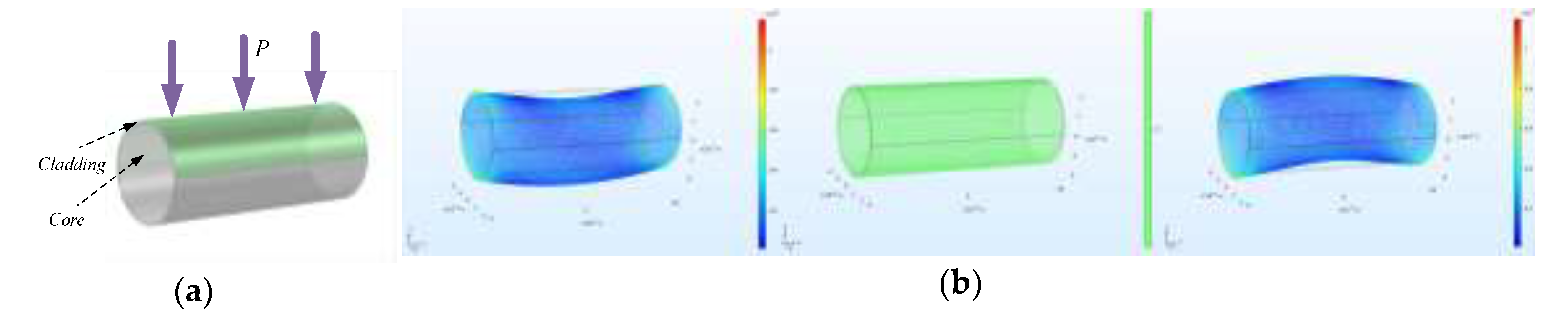
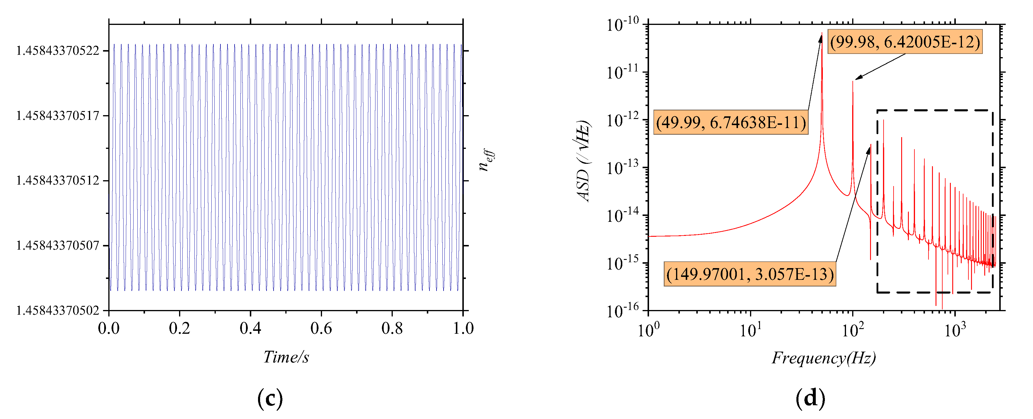
2.2. Simulations
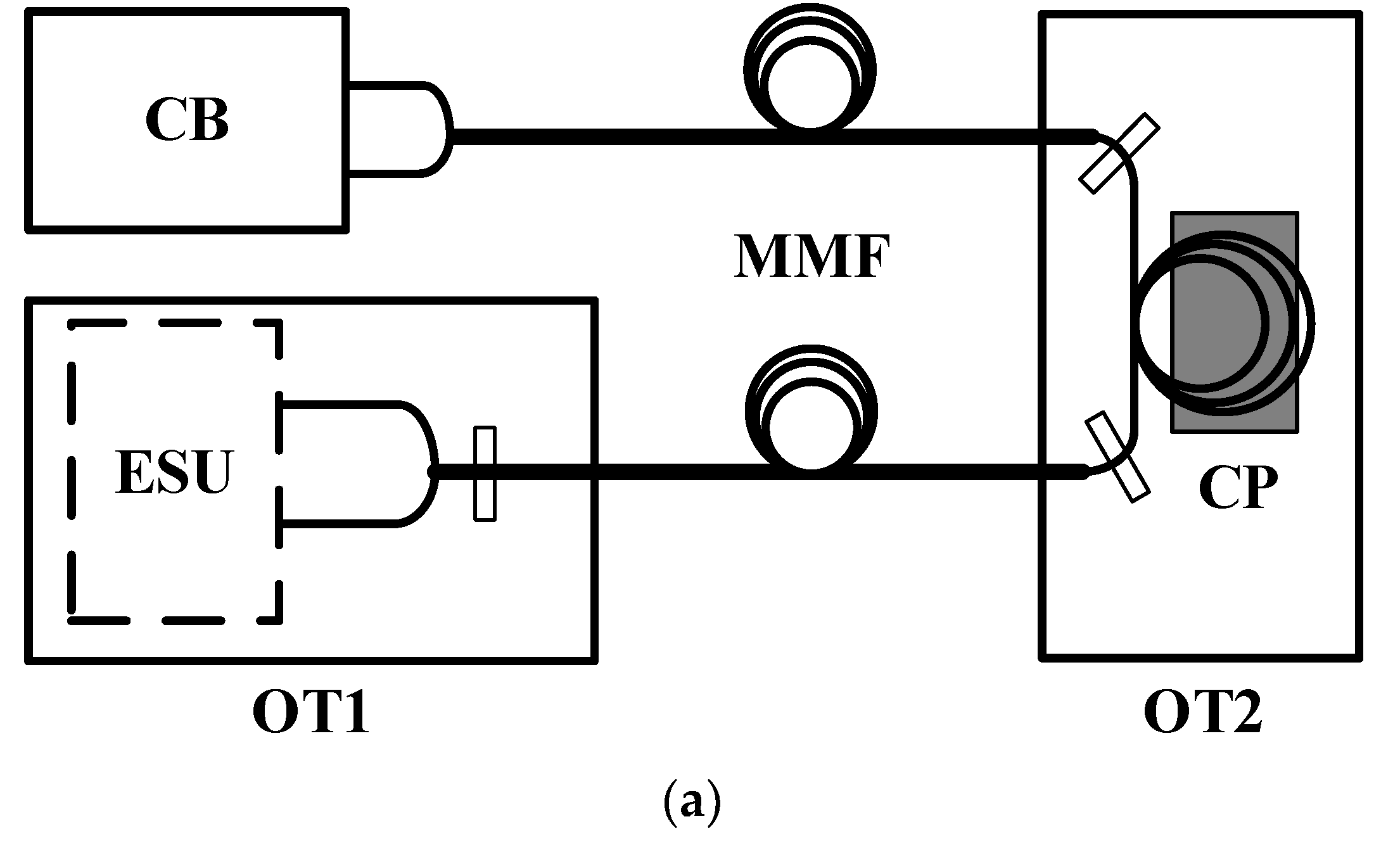
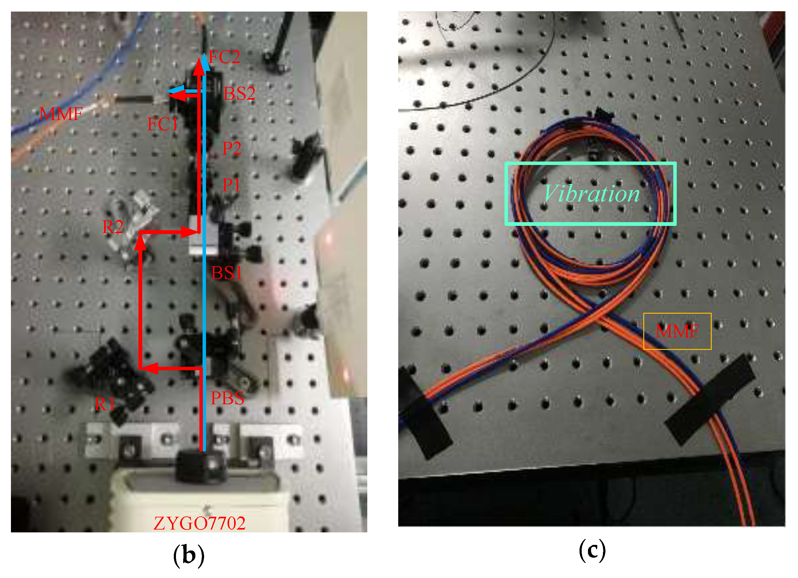
3. Experiments
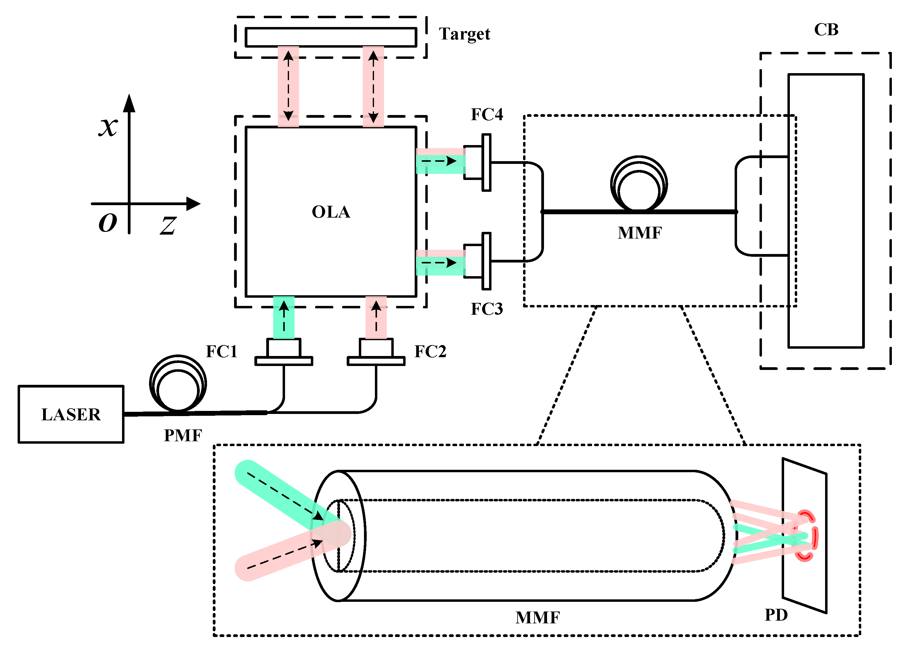
3.1. Experimental Principle
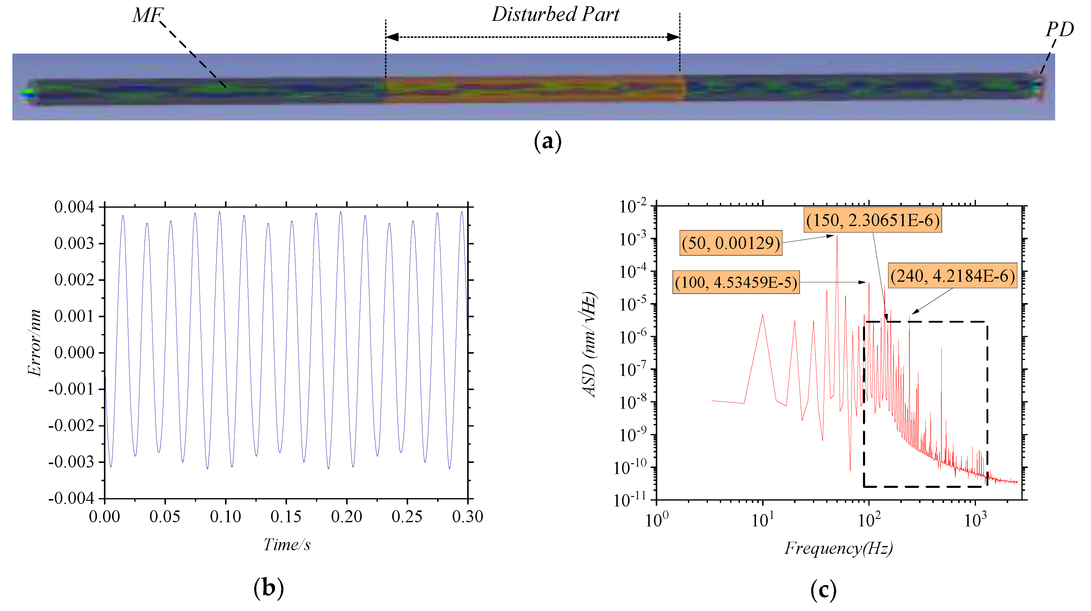
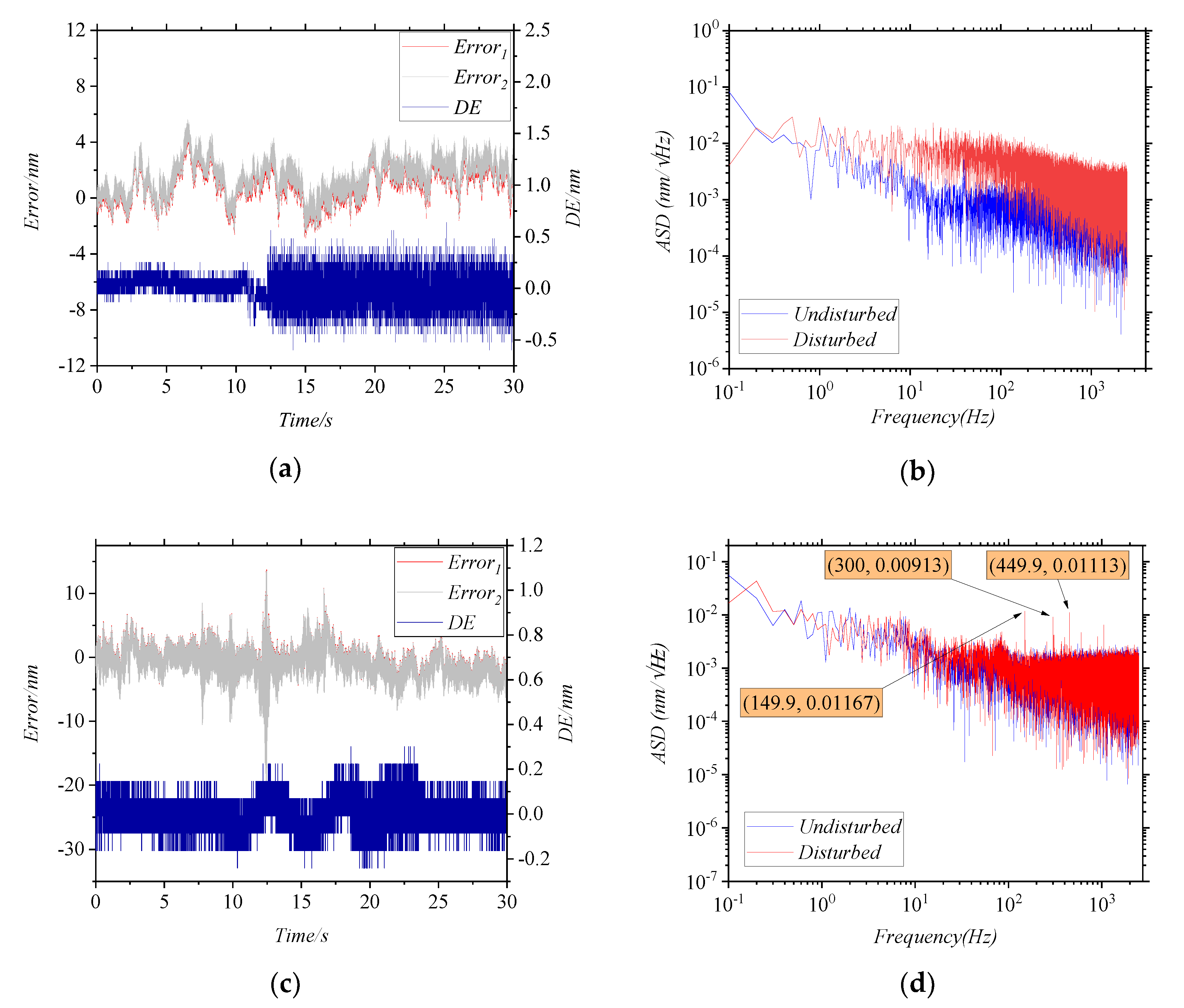
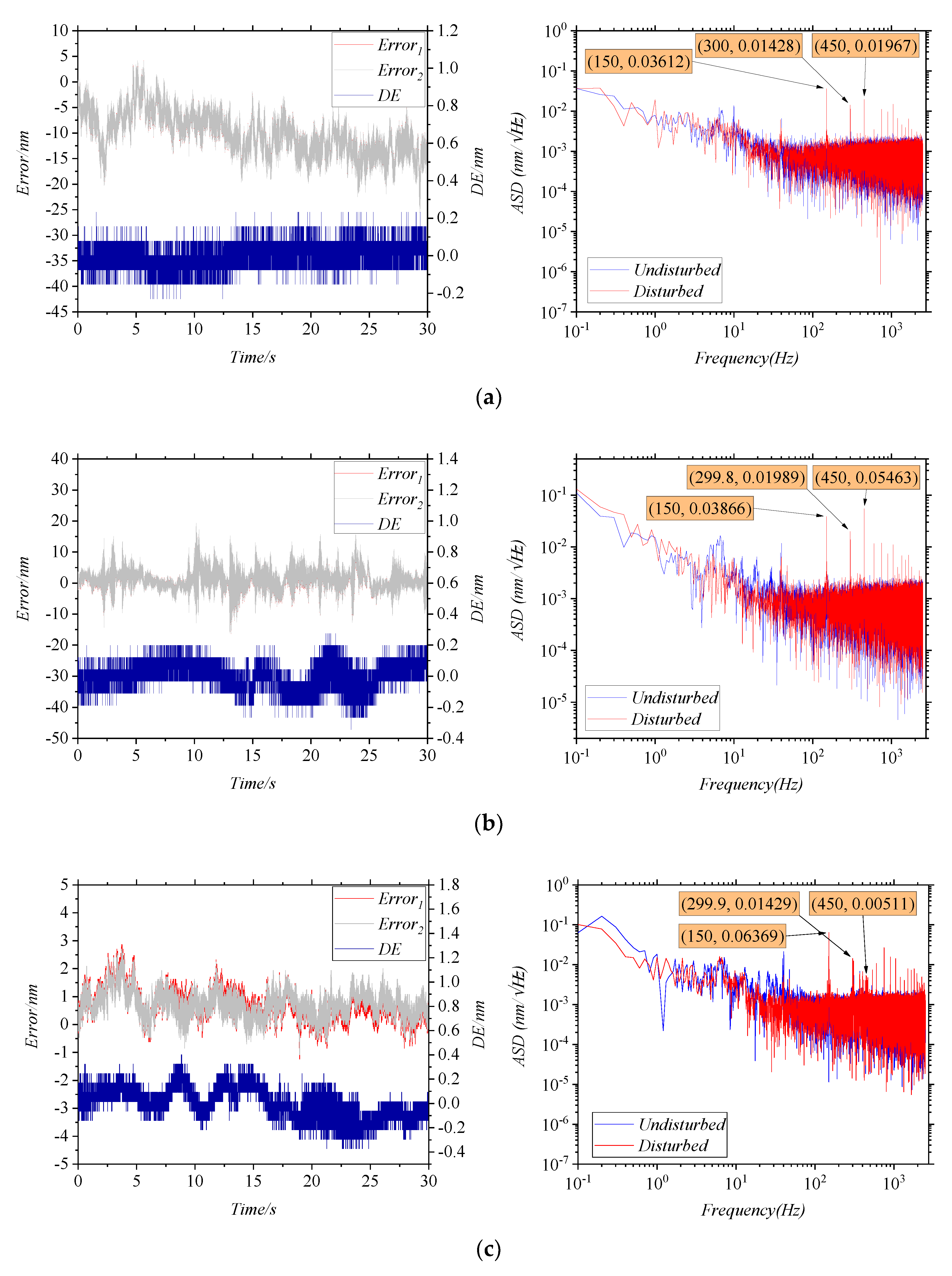
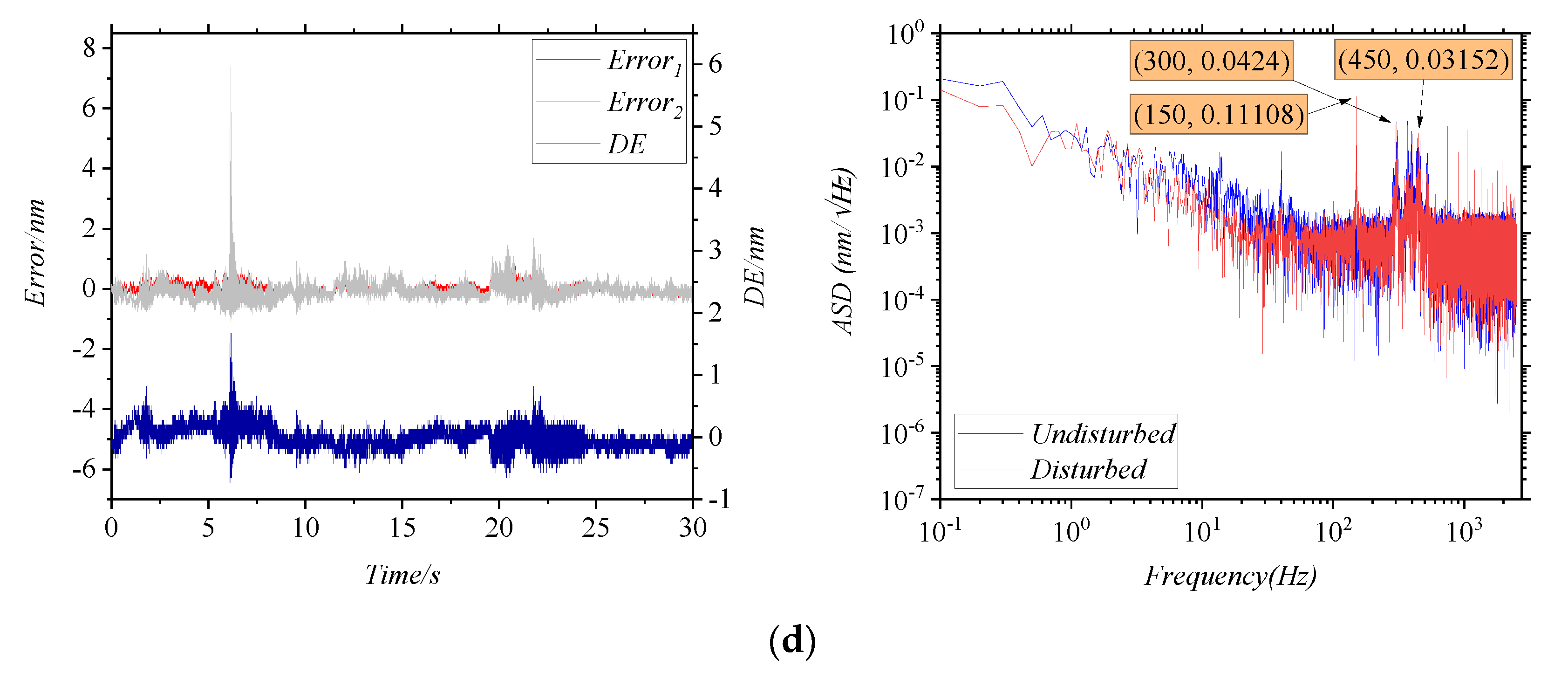
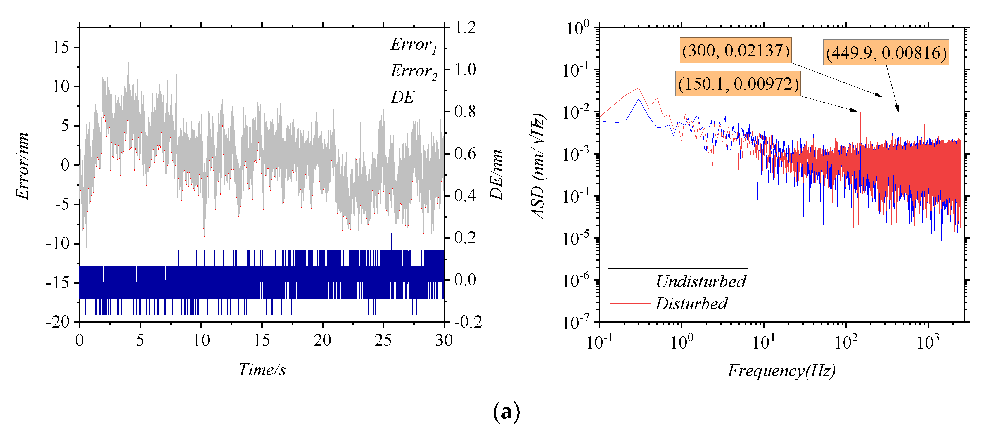
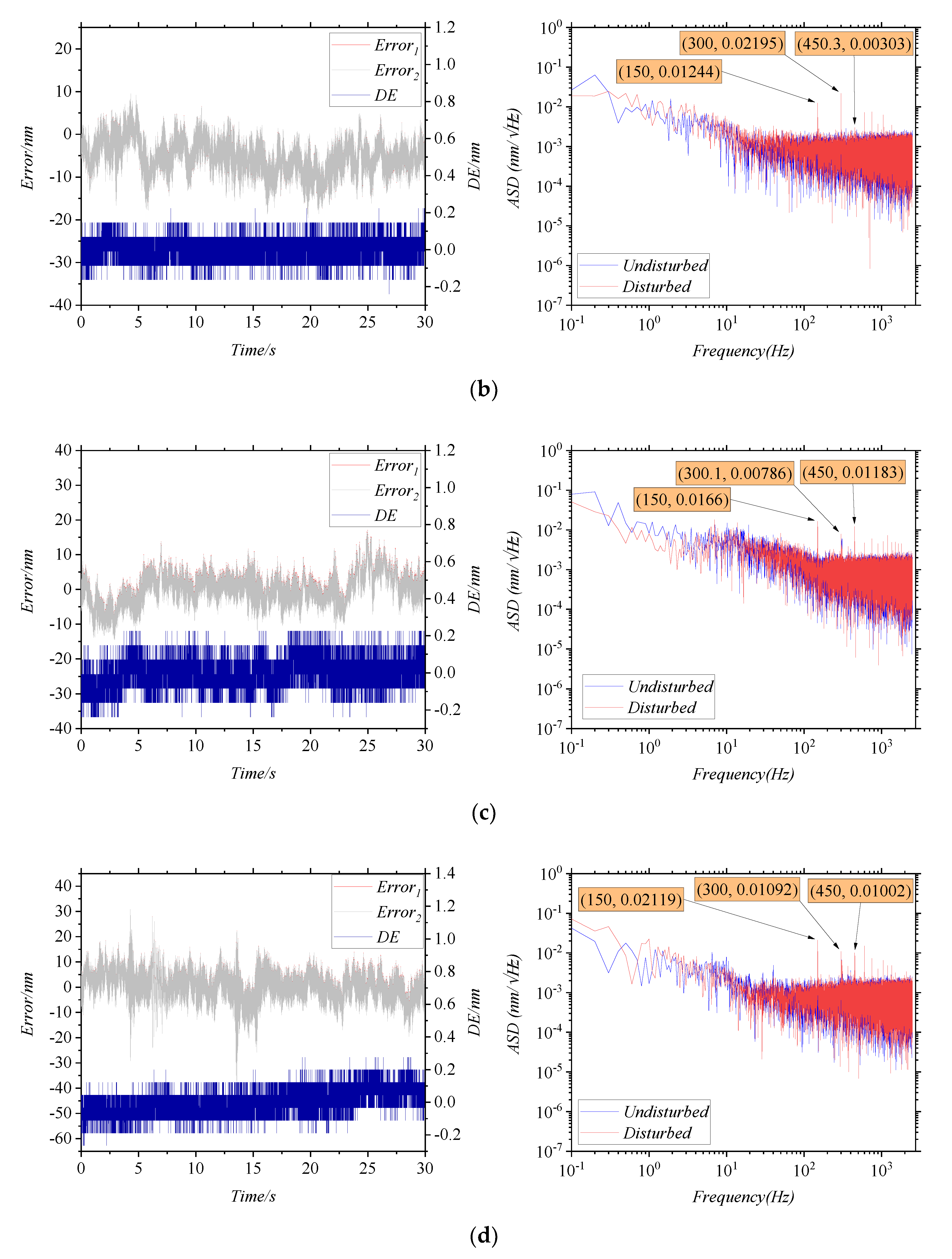
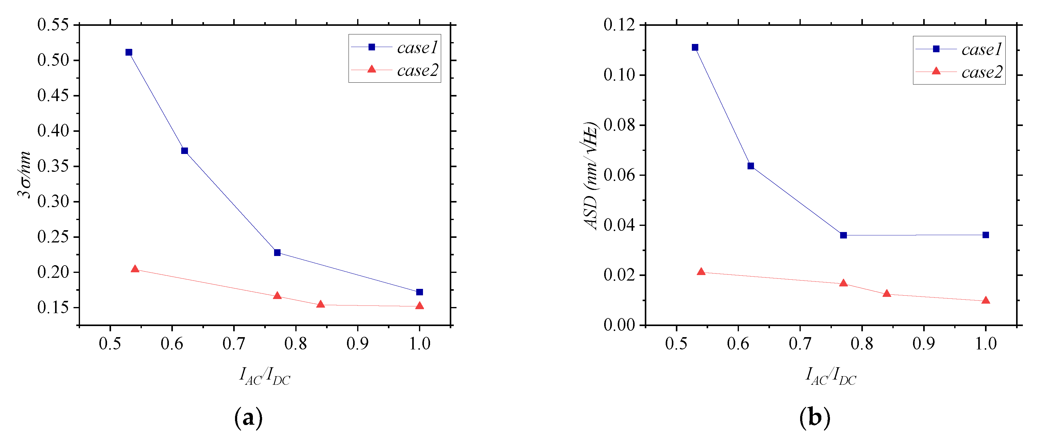
3.2. Results and Analysis
4. Conclusions
Author Contributions
Funding
Acknowledgments
Conflicts of Interest
References
- Knarren, B.A.; Cosijns, S.J.; Haitjema, H.; Schellekens, P.H. Fiber characterization for application in heterodyne laser interferometry with nanometer uncertainty, part I: Polarization state measurements. Opt. Eng. 2005, 44, 025002. [Google Scholar] [CrossRef]
- Knarren, B.A.; Cosijns, S.J.; Haitjema, H.; Schellekens, P.H. Fiber characterization for application in heterodyne laser interferometry, part II: Modeling and analysis. Opt. Eng. 2005, 44, 025003. [Google Scholar] [CrossRef]
- Ellis, J.D.; Meskers, A.J.; Spronck, J.W.; Schmidt, R.H.M. Fiber-coupled displacement interferometry without periodic nonlinearity. Opt. Lett. 2011, 36, 3584–3586. [Google Scholar] [CrossRef] [PubMed] [Green Version]
- Meskers, A.J.; Spronck, J.W.; Schmidt, R.H.M. Validation of separated source frequency delivery for a fiber-coupled heterodyne displacement interferometer. Opt. Lett. 2014, 39, 4603–4606. [Google Scholar] [CrossRef] [Green Version]
- Yang, F.; Zhang, M.; Ye, W.; Wang, L. Three-degrees-of-freedom laser interferometer based on differential wavefront sensing with wide angular measurement range. Appl. Opt. 2019, 58, 723–728. [Google Scholar] [CrossRef]
- Ye, W.; Zhang, M.; Zhu, Y.; Wang, L.; Hu, J.; Li, X.; Hu, C. Translational displacement computational algorithm of the grating interferometer without geometric error for the wafer stage in a photolithography scanner. Opt. Express 2018, 26, 34734–34752. [Google Scholar] [CrossRef]
- Yang, F.; Zhang, M.; Zhu, Y.; Ye, W.; Wang, L.; Xia, Y. Two Degree-of-Freedom Fiber-Coupled Heterodyne Grating Interferometer with Milli-Radian Operating Range of Rotation. Sensors 2019, 19, 3219. [Google Scholar] [CrossRef] [Green Version]
- Agrawal, G.P.; Mumtaz, S.; Essiambre, R.-J. Nonlinear performance of SDM systems designed with multimode or multicore fibers. In Proceedings of the Optical Fiber Communication Conference, Anaheim, CA, USA, 17–21 March 2013. [Google Scholar]
- Mumtaz, S.; Essiambre, R.-J.; Agrawal, G.P. Reduction of nonlinear penalties due to linear coupling in multicore optical fibers. IEEE Photonics Technol. Lett. 2012, 24, 1574–1576. [Google Scholar] [CrossRef]
- San Fabián, N.; Socorro-Leránoz, A.B.; Del Villar, I.; Díaz, S.; Matías, I.R. Multimode-coreless-multimode fiber-based sensors: Theoretical and experimental study. J. Lightwave Technol. 2019, 37, 3844–3850. [Google Scholar] [CrossRef]
- Zhang, S.; Deng, S.; Wang, Z.; Yang, W.; Sun, C.; Chen, X.; Ma, Y.; Li, Y.; Geng, T.; Sun, W. Optimization and experiment of a miniature multimode fiber induced-LPG refractometer. OSA Contin. 2019, 2, 2190–2198. [Google Scholar] [CrossRef]
- Fermann, M.E. Single-mode excitation of multimode fibers with ultrashort pulses. Opt. Lett. 1998, 23, 52–54. [Google Scholar] [CrossRef] [PubMed]
- Gloge, D.; Marcatili, E.A.J. Multimode theory of graded-core fibers. Bell Syst. Tech. J. 1973, 52, 1563–1578. [Google Scholar] [CrossRef]
- Koplow, J.P.; Kliner, D.A.; Goldberg, L. Single-mode operation of a coiled multimode fiber amplifier. Opt. Lett. 2000, 25, 442–444. [Google Scholar] [CrossRef] [PubMed] [Green Version]
- Poletti, F.; Horak, P. Description of ultrashort pulse propagation in multimode optical fibers. IOSA B 2008, 25, 1645–1654. [Google Scholar] [CrossRef]
- Hansen, T.P.; Broeng, J.; Libori, S.E.; Knudsen, E.; Bjarklev, A.; Jensen, J.R.; Simonsen, H. Highly birefringent index-guiding photonic crystal fibers. IEEE Photonics Technol. Lett. 2001, 13, 588–590. [Google Scholar] [CrossRef] [Green Version]
- Schriemer, H.P.; Cada, M. Modal birefringence and power density distribution in strained buried-core square waveguides. IEEE J. Quantum Electron. 2004, 40, 1131–1139. [Google Scholar] [CrossRef]
- Stone, J. Stress-optic effects, birefringence, and reduction of birefringence by annealing in fiber Fabry-Perot interferometers. J. Lightwave Technol. 1988, 6, 1245–1248. [Google Scholar] [CrossRef]
- Hsu, C.-C.; Chen, H.; Chiang, C.-W.; Chang, Y.-W.J.O.e. Dual displacement resolution encoder by integrating single holographic grating sensor and heterodyne interferometry. Opt. Express 2017, 25, 30189–30202. [Google Scholar] [CrossRef]
- Jiang, M.L.; Li, F.P.; Wang, X.D. Mini-nano-displacement measurement with double diffraction grating. Adv. Mater. Res. 2011, 230–232, 1159–1163. [Google Scholar] [CrossRef]
- Lee, C.; Lee, S.-K. Multi-degree-of-freedom motion error measurement in an ultraprecision machine using laser encoder. J. Mech. Sci. Technol. 2013, 27, 141–152. [Google Scholar] [CrossRef]
- Lin, C.; Yan, S.; Ding, D.; Wang, G. Two-dimensional diagonal-based heterodyne grating interferometer with enhanced signal-to-noise ratio and optical subdivision. Opt. Eng. 2018, 57, 064102. [Google Scholar] [CrossRef]
- Lu, Z.; Wei, P.; Wang, C.; Jing, J.; Tan, J.; Zhao, X. Two-degree-of-freedom displacement measurement system based on double diffraction gratings. Meas. Sci. Technol. 2016, 27, 074012. [Google Scholar] [CrossRef]
- Wang, X.; Dong, X.; Guo, J.; Xie, T. Two-dimensional displacement sensing using a cross diffraction grating scheme. J. Opt. A Pure Appl. Opt. 2003, 6, 106. [Google Scholar] [CrossRef]
- Castenmiller, T.; van de Mast, F.; de Kort, T.; van de Vin, C.; de Wit, M.; Stegen, R.; van Cleef, S. Towards ultimate optical lithography with NXT: 1950i dual stage immersion platform. In Proceedings of the Optical Microlithography XXIII, San Jose, CA, USA, 12 March 2010. [Google Scholar]
- Ellis, J.D. Field Guide to Displacement Measuring Interferometry; SPIE Press: Bellingham, UK, 2014; pp. 9–12. [Google Scholar]


| Parameters | Value | Description |
|---|---|---|
| λ | 633 nm | Free space wavelength |
| n1 | 1.3982 | Refractive index of the cladding |
| n2 | 1.4584 | Refractive index of the core |
| d1 | 425 μm | Outer diameter of the cladding |
| d1 | 400 μm | Diameter of the core |
| L | 1 mm | Length of MMF |
| E | 78 GPa | Young’s modulus |
| ρ | 2203 kg/m3 | Density |
| μ | 0.17 | Poisson’s ratio |
| B1 | 0.65 × 10⁻¹² m2/N | First stress optical coefficient |
| B2 | 4.2 × 10⁻¹² m2/N | Second stress optical coefficient |
© 2020 by the authors. Licensee MDPI, Basel, Switzerland. This article is an open access article distributed under the terms and conditions of the Creative Commons Attribution (CC BY) license (http://creativecommons.org/licenses/by/4.0/).
Share and Cite
Xia, Y.; Zhang, M.; Zhu, Y.; Ye, W.; Yang, F.; Wang, L. Analysis of the Errors Caused by Disturbed Multimode Fibers in the Interferometer with Fiber-Coupled Delivery. Sensors 2020, 20, 1513. https://doi.org/10.3390/s20051513
Xia Y, Zhang M, Zhu Y, Ye W, Yang F, Wang L. Analysis of the Errors Caused by Disturbed Multimode Fibers in the Interferometer with Fiber-Coupled Delivery. Sensors. 2020; 20(5):1513. https://doi.org/10.3390/s20051513
Chicago/Turabian StyleXia, Yizhou, Ming Zhang, Yu Zhu, Weinan Ye, Fuzhong Yang, and Leijie Wang. 2020. "Analysis of the Errors Caused by Disturbed Multimode Fibers in the Interferometer with Fiber-Coupled Delivery" Sensors 20, no. 5: 1513. https://doi.org/10.3390/s20051513