Two-Stream Attention Network for Pain Recognition from Video Sequences


Abstract
:
1. Introduction
2. Related Work
3. Proposed Approach
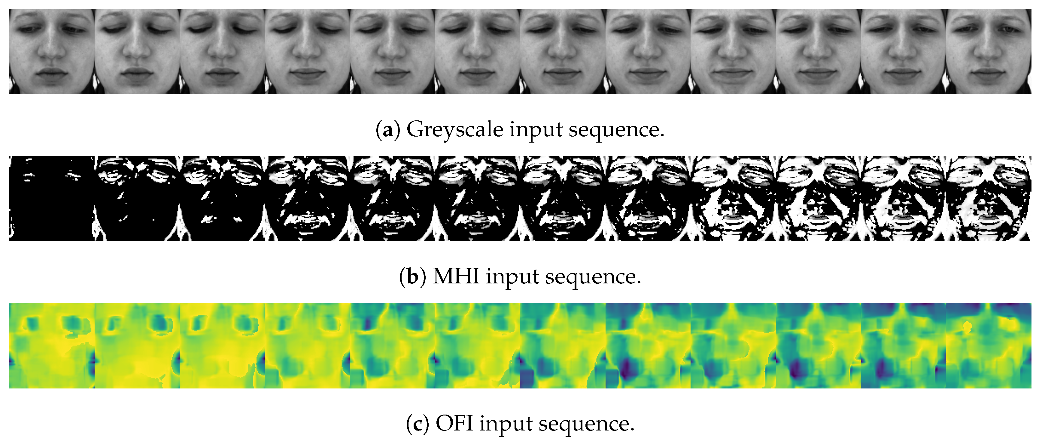
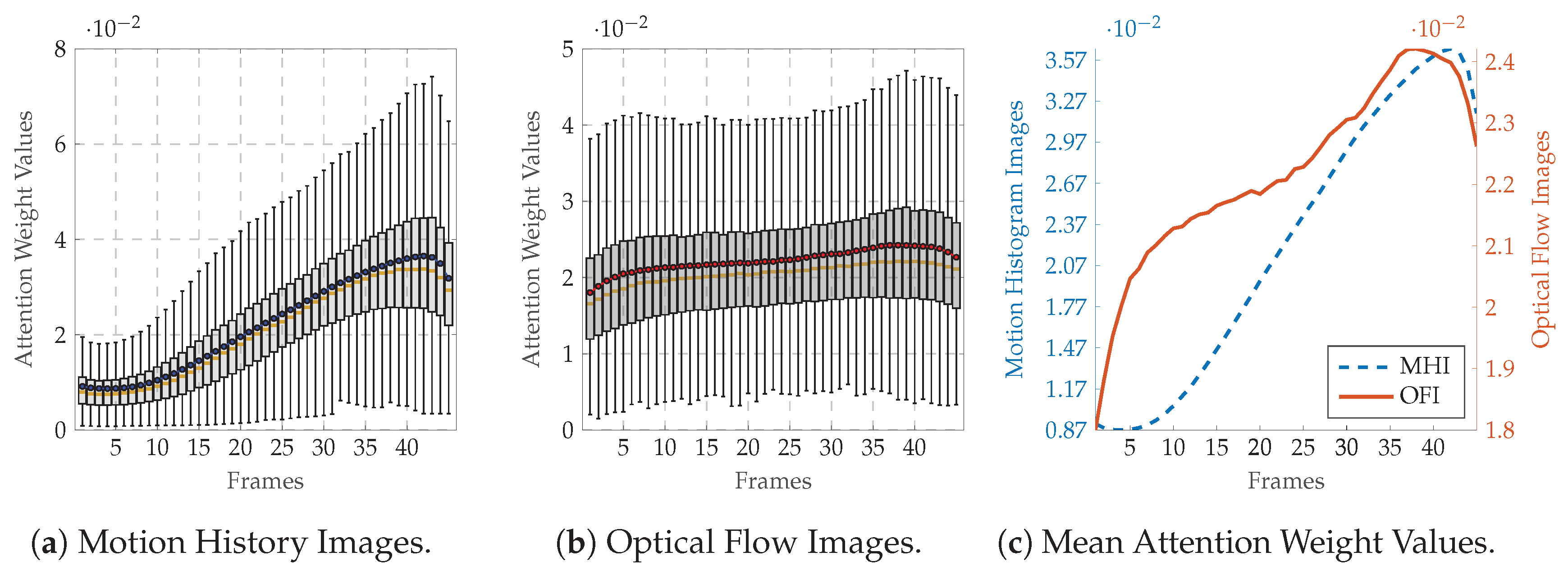
3.1. Motion History Image (MHI)
3.2. Optical Flow Image (OFI)
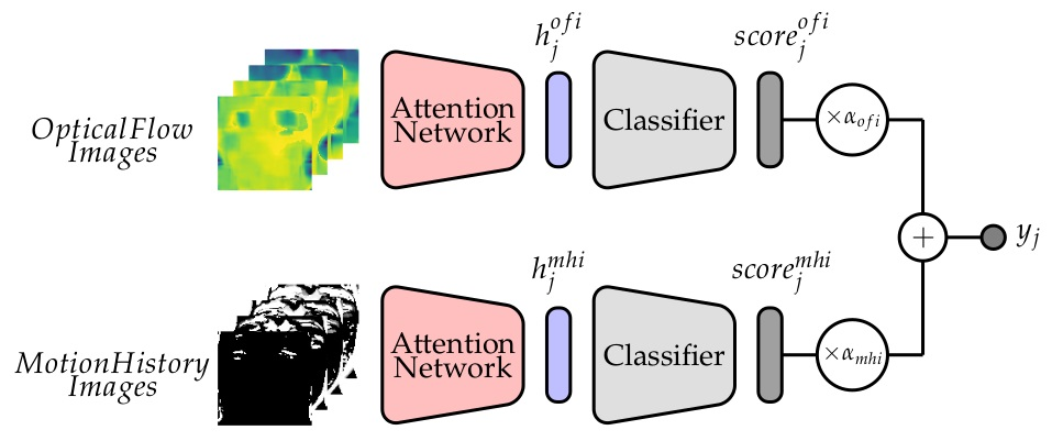
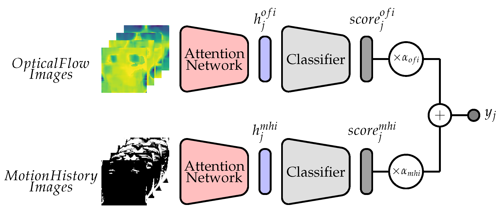
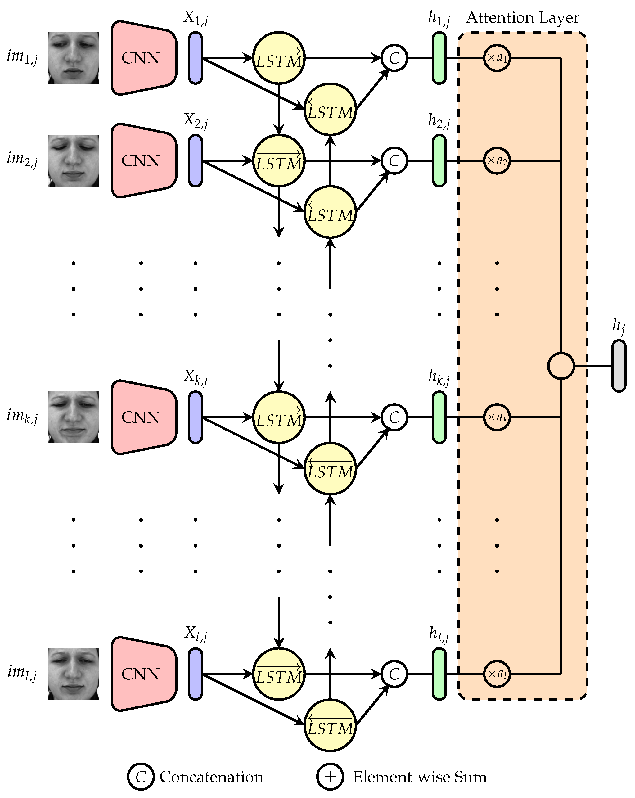
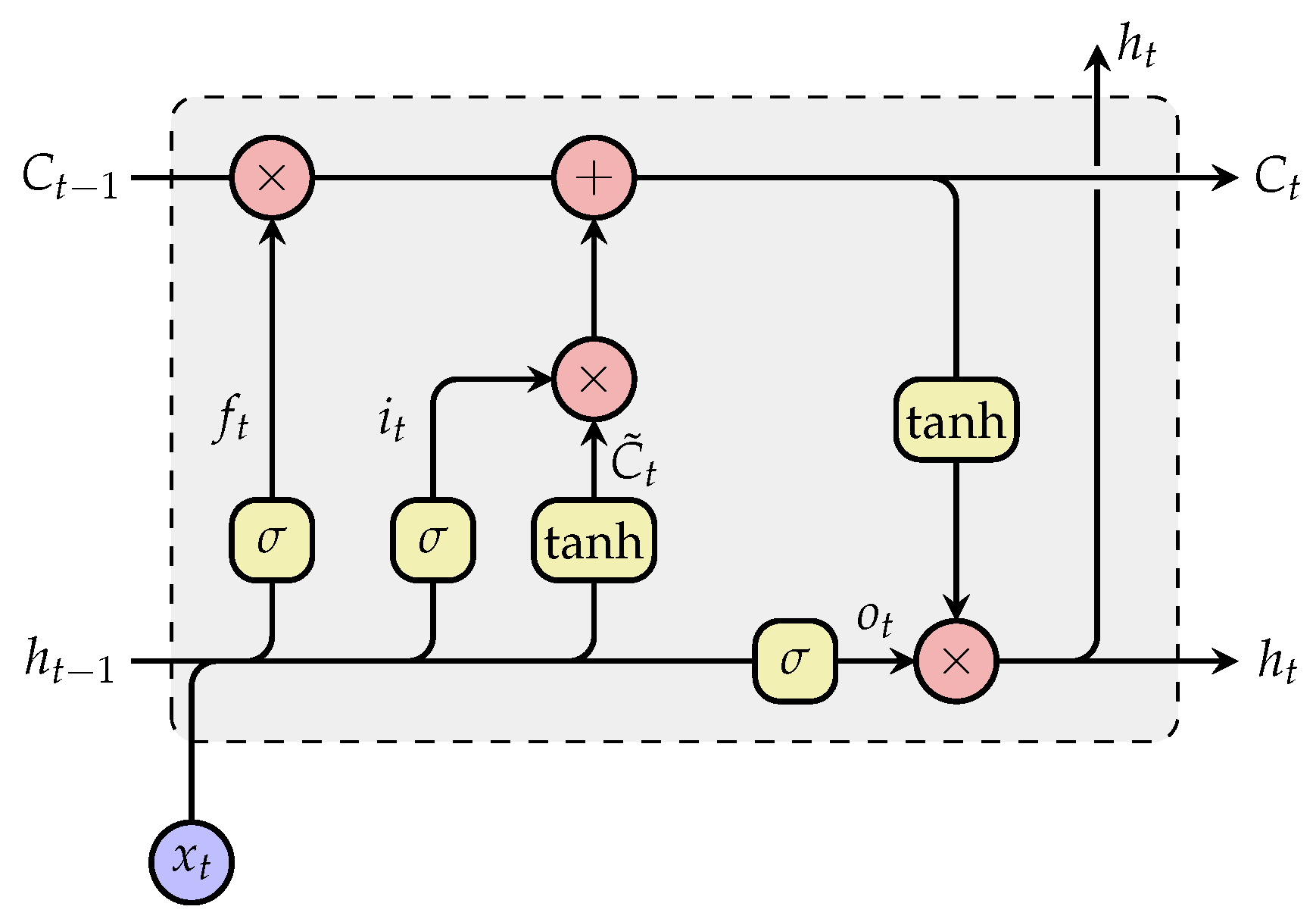
3.3. Network Architecture
4. Experiments
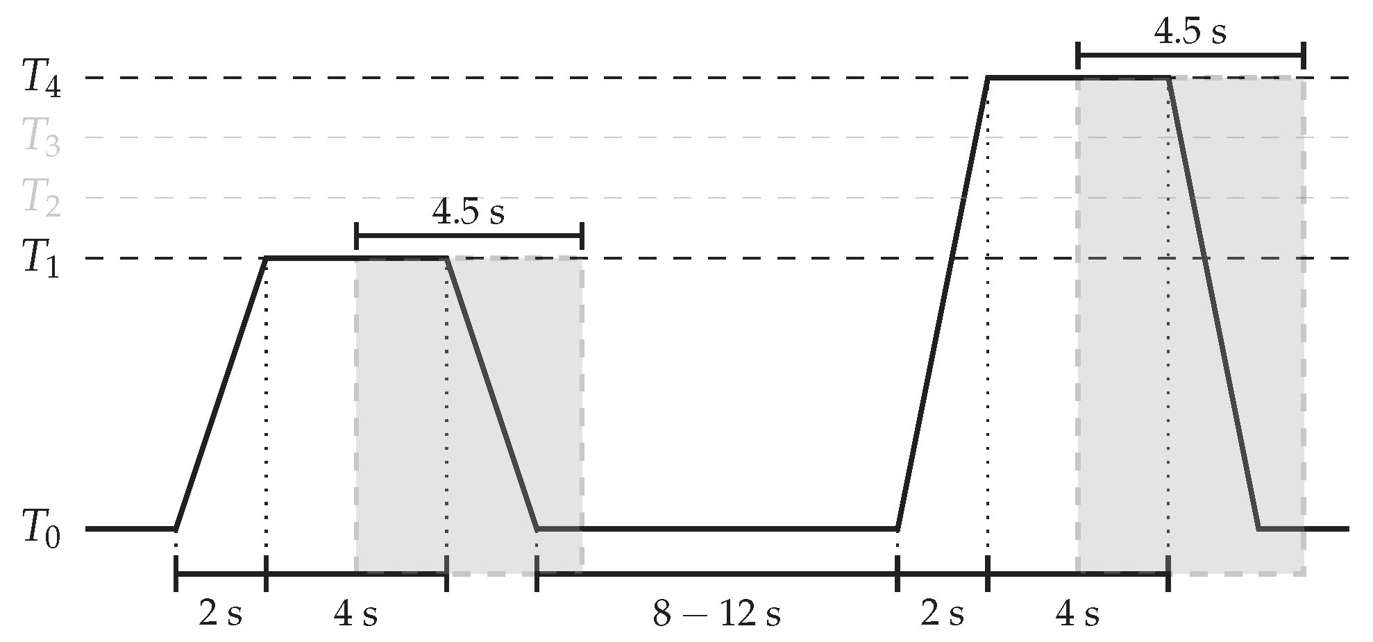
4.1. Datasets Description
4.2. Data Preprocessing
4.3. Experimental Settings
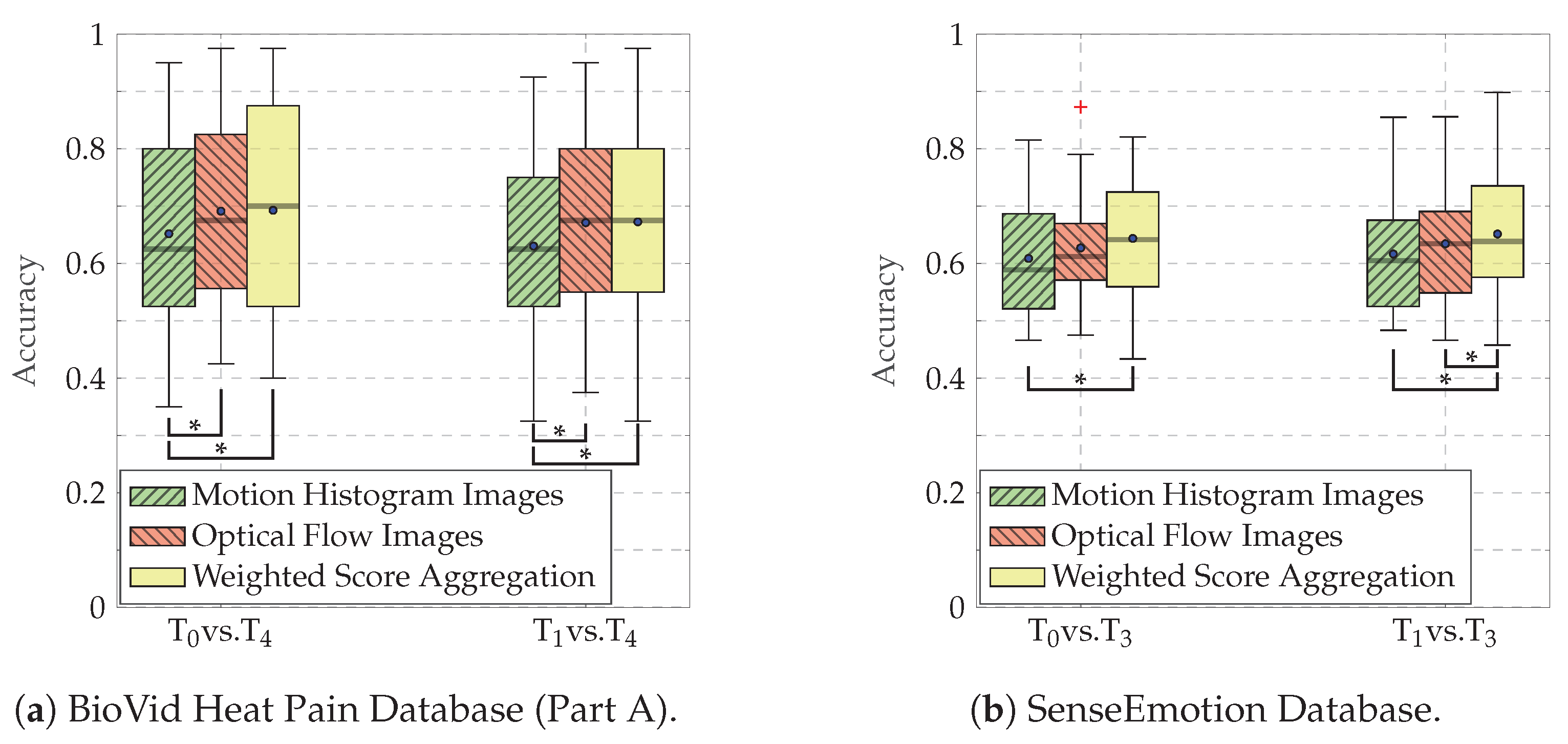
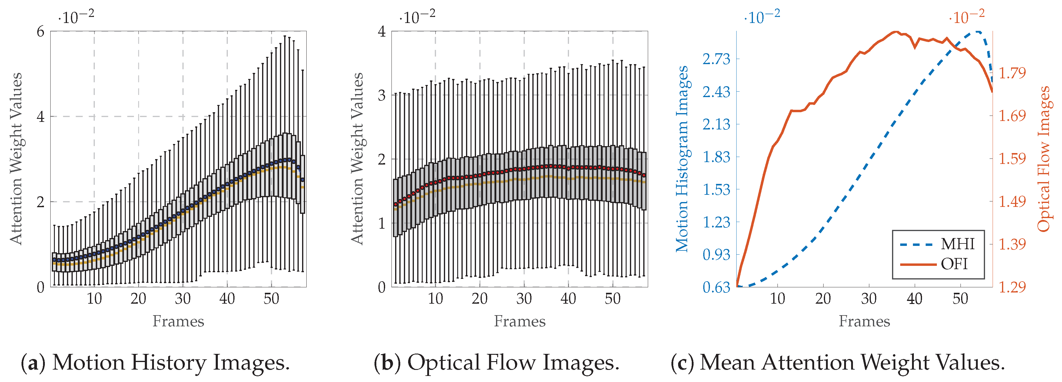
4.4. Results
5. Conclusions
Author Contributions
Funding
Acknowledgments
Conflicts of Interest
References
- Ahad, M.A.R.; Tan, J.K.; Kim, H.; Ishikawa, S. Motion History Image: its variants and applications. Mach. Vis. Appl. 2012, 23, 255–281. [Google Scholar] [CrossRef]
- Horn, B.K.P.; Schunck, B.G. Determining optical flow. Artif. Intell. 1981, 17, 185–203. [Google Scholar] [CrossRef] [Green Version]
- Lucey, P.; Cohn, J.F.; Prkachin, K.M.; Solomon, P.E.; Matthews, I. Painful data: The UNBC-McMaster shoulder pain expression archive database. In Proceedings of the Face and Gesture, Santa Barbara, CA, USA, 21–25 March 2011; pp. 57–64. [Google Scholar]
- Walter, S.; Gruss, S.; Ehleiter, H.; Tan, J.; Traue, H.C.; Crawcour, S.; Werner, P.; Al-Hamadi, A.; Andrade, A. The BioVid heat pain database data for the advancement and systematic validation of an automated pain recognition system. In Proceedings of the IEEE International Conference on Cybernetics, Lausanne, Switzerland, 13–15 June 2013; pp. 128–131. [Google Scholar]
- Aung, M.S.H.; Kaltwang, S.; Romera-Paredes, B.; Martinez, B.; Singh, A.; Cella, M.; Valstar, M.; Meng, H.; Kemp, A.; Shafizadeh, M.; et al. The automatic detection of chronic pain-related expression: requirements, challenges and multimodal dataset. IEEE Trans. Affect. Comput. 2016, 7, 435–451. [Google Scholar] [CrossRef] [PubMed] [Green Version]
- Velana, M.; Gruss, S.; Layher, G.; Thiam, P.; Zhang, Y.; Schork, D.; Kessler, V.; Gruss, S.; Neumann, H.; Kim, J.; et al. The SenseEmotion Database: A multimodal database for the development and systematic validation of an automatic pain- and emotion-recognition system. In Proceedings of the Multimodal Pattern Recognition of Social Signals in Human-Computer-Interaction, Cancun, Mexico, 4 December 2016; pp. 127–139. [Google Scholar]
- Thiam, P.; Kessler, V.; Schwenker, F. Hierarchical combination of video features for personalised pain level recognition. In Proceedings of the 25th European Symposium on Artificial Neural Networks, Computational Intelligence and Machine Learning, Bruges, Belgium, 26–28 April 2017; pp. 465–470. [Google Scholar]
- Werner, P.; Al-Hamadi, A.; Limbrecht-Ecklundt, K.; Walter, S.; Gruss, S.; Traue, H.C. Automatic Pain Assessment with Facial Activity Descriptors. IEEE Trans. Affect. Comput. 2017, 8, 286–299. [Google Scholar] [CrossRef]
- Tsai, F.S.; Hsu, Y.L.; Chen, W.C.; Weng, Y.M.; Ng, C.J.; Lee, C.C. Toward Development and Evaluation of Pain Level-Rating Scale For Emergency Triage Based on Vocal Characteristics and Facial Expressions. In Proceedings of the Interspeech 2016, San-Francisco, CA, USA, 8–12 September 2016; pp. 92–96. [Google Scholar]
- Thiam, P.; Schwenker, F. Combining deep and hand-crafted features for audio-based pain intensity classification. In Proceedings of the Multimodal Pattern Recognition of Social Signals in Human-Computer- Interaction, Beijing, China, 20 August 2018; pp. 49–58. [Google Scholar]
- Walter, S.; Gruss, S.; Limbrecht-Ecklundt, K.; Traue, H.C.; Werner, P.; Al-Hamadi, A.; Diniz, N.; Silva, G.M.; Andrade, A.O. Automatic pain quantification using autonomic parameters. Psych. Neurosci. 2014, 7, 363–380. [Google Scholar] [CrossRef] [Green Version]
- Chu, Y.; Zhao, X.; Han, J.; Su, Y. Physiological signal-based method for measurement of pain intensity. Front. Neurosci. 2017, 11, 279. [Google Scholar] [CrossRef]
- Lopez-Martinez, D.; Picard, R. Continuous pain intensity estimation from autonomic signals with recurrent neural networks. In Proceedings of the 40th Annual International Conference of the IEEE Engineering in Medecine and Biology Society, Honolulu, HI, USA, 18–21 July 2018; pp. 5624–5627. [Google Scholar]
- Thiam, P.; Schwenker, F. Multi-modal data fusion for pain intensity assessement and classification. In Proceedings of the 7th International Conference on Image Processing Theory, Tools and Applications, Montreal, QC, Canada, 28 November–1 December 2017; pp. 1–6. [Google Scholar]
- Thiam, P.; Kessler, V.; Amirian, M.; Bellmann, P.; Layher, G.; Zhang, Y.; Velana, M.; Gruss, S.; Walter, S.; Traue, H.C.; et al. Multi-modal pain intensity recognition based on the SenseEmotion Database. IEEE Trans. Affect. Comput. 2019. [Google Scholar] [CrossRef]
- Thiam, P.; Bellmann, P.; Kestler, H.A.; Schwenker, F. Exploring deep physiological models for nociceptive pain recognition. Sensors 2019, 19, 4503. [Google Scholar] [CrossRef] [Green Version]
- Ekman, P.; Friesen, W.V. The Facial Action Unit System: A Technique for the Measurement of Facial Movement; Consulting Psychologist Press: Mountain View, CA, USA, 1978. [Google Scholar]
- Senechal, T.; McDuff, D.; Kaliouby, R.E. Facial Action Unit detection using active learning and an efficient non-linear kernel approximation. In Proceedings of the IEEE International Conference on Computer Vision Workshop, Santiago, Chile, 7–13 December 2015; pp. 10–18. [Google Scholar]
- Lucey, P.; Cohn, J.; Lucey, S.; Matthews, I.; Sridharan, S.; Prkachin, K.M. Automatically detecting pain using Facial Actions. In Proceedings of the 3rd International Conference on Affective Computing and Intelligent Interaction and Workshops, Amsterdam, The Netherlands, 10–12 September 2009; pp. 1–8. [Google Scholar]
- Abe, S. Support Vector Machines for Pattern Classification; Springer: Berlin, Germany, 2005. [Google Scholar]
- Brümmer, N.; Preez, J.D. Application-independent evaluation of speaker detection. Comput. Speech Lang. 2006, 20, 230–275. [Google Scholar] [CrossRef]
- Zafar, Z.; Khan, N.A. Pain intensity evaluation through Facial Action Units. In Proceedings of the 22nd International Conference on Pattern Recognition, Stockholm, Sweden, 24–28 August 2014; pp. 4696–4701. [Google Scholar]
- Cover, T.; Hart, P. Nearest Neighbor Pattern Classification. IEEE Trans. Inf. Theory 1967, 13, 21–27. [Google Scholar] [CrossRef]
- Prkachin, K.M.; Solomom, P.E. The structure, reliability and validity of pain expression: Evidence from patients with shoulder pain. Pain 2008, 139, 267–274. [Google Scholar] [CrossRef]
- Xu, X.; Craig, K.D.; Diaz, D.; Goodwin, M.S.; Akcakaya, M.; Susam, B.T.; Huang, J.S.; de Sa, V.S. Automated pain detection in facial videos of children using human-assisted transfer learning. In Proceedings of the International Workshop on Artificial Intelligence in Health, Stockholm, Sweden, 13–14 July 2018; pp. 162–180. [Google Scholar]
- Monwar, M.; Rezaei, S. Pain recognition using artificial neural network. In Proceedings of the IEEE International Symposium on Signal Processing and Information Theory, Vancouver, BC, Canada, 27–30 August 2006; pp. 8–33. [Google Scholar]
- Yang, R.; Tong, S.; Bordallo, M.; Boutellaa, E.; Peng, J.; Feng, X.; Hadid, A. On pain assessment from facial videos using spatio-temporal local descriptors. In Proceedings of the 6th International Conference on Image Processing Theory, Tools and Applications, Oulu, Finland, 12–15 December 2016; pp. 1–6. [Google Scholar]
- Zhao, G.; Pietikaeinen, M. Dynamic texture recognition using local binary patterns with an application to facial expressions. IEEE Trans. Pattern Anal. Mach. Intell. 2007, 29, 915–928. [Google Scholar] [CrossRef] [Green Version]
- Ojansivu, V.; Heikkilä, J. Blur insensitive texture classification using local phase quantization. In Proceedings of the Image and Signal Processing, Cherbourg-Octeville, France, 1–3 July 2008; pp. 236–243. [Google Scholar]
- Kannala, J.; Rahtu, E. BSIF: Binarized Statistical Image Features. In Proceedings of the 21st International Conference on Pattern Recognition, Tsukuba, Japan, 11–15 November 2012; pp. 1363–1366. [Google Scholar]
- Kächele, M.; Thiam, P.; Amirian, M.; Werner, P.; Walter, S.; Schwenker, F.; Palm, G. Engineering Applications of Neural Networks. Multimodal data fusion for person-independent, continuous estimation of pain Intensity. In Proceedings of the Engineering Applications of Neural Networks, Rhodes, Greece, 25–28 September 2015; pp. 275–285. [Google Scholar]
- Breiman, L. Random Forests. Mach. Learn. 2001, 45, 5–32. [Google Scholar] [CrossRef] [Green Version]
- Thiam, P.; Kessler, V.; Walter, S.; Palm, G.; Scwenker, F. Audio-visual recognition of pain intensity. In Proceedings of the Multimodal Pattern Recognition of Social Signals in Human-Computer-Interaction, Cancun, Mexico, 4 December 2016; pp. 110–126. [Google Scholar]
- Bosch, A.; Zisserman, A.; Munoz, X. Representing shape with a spatial pyramid kernel. In Proceedings of the 6th ACM International Conference on Image and Video Retrieval, Amsterdam, The Netherlands, 9–11 July 2007; pp. 401–408. [Google Scholar]
- Almaev, T.R.; Valstar, M.F. Local Gabor Binary Patterns from Three Orthogonal Planes for automatic facial expression recognition. In Proceedings of the 2013 Humaine Association Conference on Affective Computing and Intelligent Interaction, Geneva, Switzerland, 2–5 September 2013; pp. 356–361. [Google Scholar]
- Bellantonio, M.; Haque, M.A.; Rodriguez, P.; Nasrollahi, K.; Telve, T.; Guerrero, S.E.; Gonzàlez, J.; Moeslund, T.B.; Rasti, P.; Anbarjafari, G. Spatio-temporal pain recognition in CNN-based super-resolved facial images. In Proceedings of the International Conference on Pattern Recognition: Workshop on Face and Facial Expression Recognition, Cancun, Mexico, 4 December 2016; pp. 151–162. [Google Scholar]
- Rodriguez, P.; Cucurull, G.; Gonzàlez, J.; Gonfaus, J.M.; Nasrollahi, K.; Moeslund, T.B.; Roca, F.X. Deep Pain: Exploiting Long Short-Term Memory networks for facial expression classification. IEEE Trans. Cybern. 2018. [Google Scholar] [CrossRef] [Green Version]
- Kalischek, N.; Thiam, P.; Bellmann, P.; Schwenker, F. Deep domain adaptation for facial expression analysis. In Proceedings of the 8th International Conference on Affective Computing and Intelligent Interaction Workshops and Demos, Cambridge, UK, 3–6 September 2019; pp. 317–323. [Google Scholar]
- LeCun, Y.; Kavukcuoglu, K.; Farabet, C. Convolutional networks and application in vision. In Proceedings of the IEEE International Symposium on Circuits and Systems, 2010, Paris, France, 30 May–2 June 2010; pp. 253–256. [Google Scholar]
- Hochreiter, S.; Schmidhuber, J. Long Short-Term Memory. Neural Comput. 1997, 9, 1735–1780. [Google Scholar] [CrossRef]
- Soar, J.; Bargshady, G.; Zhou, X.; Whittaker, F. Deep learning model for detection of pain intensity from facial expression. In Proceedings of the International Conference on Smart Homes and Health Telematics, Singapore, 10–12 July 2018; pp. 249–254. [Google Scholar]
- Lafferty, J.D.; McCallum, A.; Pereira, F.C.N. Conditional Random Fields: Probabilistic models for segmenting and labeling sequence data. In Proceedings of the 18th International Conference on Machine Learning, Williams College, Williamstown, MA, USA, 28 June–1 July 2001; pp. 282–289. [Google Scholar]
- Bargshady, G.; Soar, J.; Zhou, X.; Deo, R.C.; Whittaker, F.; Wang, H. A joint deep neural network model for pain recognition from face. In Proceedings of the IEEE 4th International Conference on Computer and Communication Systems, Singapore, 23–25 February 2019; pp. 52–56. [Google Scholar]
- Zhou, J.; Hong, X.; Su, F.; Zhao, G. Recurrent convolutional neural network regression for continuous pain intensity estimation in Video. In Proceedings of the IEEE Conference on Computer Vision and Pattern Recognition Workshops, Las Vegas, NV, USA, 26 June–1 July 2016; pp. 1535–1543. [Google Scholar]
- Liang, M.; Hi, X. Recurrent convolutional neural network for object recognition. In Proceedings of the IEEE Conference on Computer Vision and Pattern Recognition, Boston, MA, USA, 7–12 June 2015; pp. 3367–3375. [Google Scholar]
- Wang, F.; Xiang, X.; Liu, C.; Tran, T.D.; Reiter, A.; Hager, G.D.; Quaon, H.; Cheng, J.; Yuille, A.L. Regularizing face verification nets for pain intensity regression. In Proceedings of the IEEE International Conference on Image Processing, Beijing, China, 17–20 September 2017; pp. 1087–1091. [Google Scholar]
- Meng, D.; Peng, X.; Wang, K.; Qiao, Y. Frame attention networks for facial expression recognition in videos. In Proceedings of the IEEE International Conference on Image Processing, Taipei, Taiwan, 22–25 September 2019; pp. 3866–3870. [Google Scholar]
- Bobick, A.F.; Davis, J.W. The recognition of human movement using temporal templates. IEEE Trans. Pattern Anal. Mach. Intell. 2001, 23, 257–267. [Google Scholar] [CrossRef] [Green Version]
- Yin, Z.; Collins, R. Moving object localization in thermal imagery by forward-backward MHI. In Proceedings of the Conference on Computer Vision and Pattern Recognition Workshop, New York, NY, USA, 17–22 June 2006; pp. 133–140. [Google Scholar]
- Farnebäck, G. Two-frame motion estimation based on polynomial expansion. In Proceedings of the Scandinavian Conference on Image Analysis, Halmstad, Sweden, 29 June–2 July 2003; pp. 363–370. [Google Scholar]
- Brox, T.; Bruhn, A.; Papenberg, N.; Weickert, J. High accuracy optical flow estimation based on a theory for warping. In Proceedings of the European Conference on Computer Vision, Prague, Czech Republic, 11–14 May 2004; pp. 25–36. [Google Scholar]
- Lucas, B.D.; Kanade, T. An iterative image registration technique with an application to stereo vision. In Proceedings of the 7th International Joint Conference on Artificial Intelligence, University of British Columbia, Vancouver, BC, Canada, 24–28 August 1981; pp. 674–679. [Google Scholar]
- Beauchemin, S.S.; Barron, J.L. The computation of optical flow. ACM Comput. Surv. 1995, 27, 433–466. [Google Scholar] [CrossRef]
- Akpinar, S.; Alpaslan, F.N. Chapter 21—Optical flow-based representation for video action detection. In Emerging Trends in Image Processing, Computer Vision and Pattern Recognition; Deligiannidis, L., Arabnia, H.R., Eds.; Morgan Kaufmann: Boston, MA, USA, 2015; pp. 331–351. [Google Scholar]
- Sun, S. A survey of multi-view machine learning. Neural Comput. Appl. 2013, 23, 2031–2038. [Google Scholar] [CrossRef]
- Schuster, M.; Paliwal, K.K. Bidirectional Recurrent Neural Network. IEEE Trans. Signal Process. 1997, 45, 2673–2681. [Google Scholar] [CrossRef] [Green Version]
- Hochreiter, S.; Bengio, Y.; Frasconi, P. Gradient flow in recurrent nets: The difficulty of learning long-term dependencies. In Field Guide to Dynamical Recurrent Networks; IEEE Press: Piscataway, NJ, USA, 2001. [Google Scholar]
- Clevert, D.A.; Unterthiner, T.; Hochreiter, S. Fast and accurate deep network learning by exponential linear units (elus). arXiv 2016, arXiv:1511.07289. Available online: https://arxiv.org/abs/1511.07289 (accessed on 3 February 2020).
- Werner, P.; Al-Hamadi, A.; Niese, R.; Walter, S.; Gruss, S.; Traue, H.C. Automatic pain recognition from video and biomedical signals. In Proceedings of the International Conference on Pattern Recognition, Stockholm, Sweden, 24–28 August 2014; pp. 4582–4587. [Google Scholar]
- Walter, S.; Gruss, S.; Traue, H.; Werner, P.; Al-Hamadi, A.; Kächele, M.; Schwenker, F.; Andrade, A.; Moreira, G. Data fusion for automated pain recognition. In Proceedings of the 9th International Conference on Pervasive Computing Technologies for Healthcare, Istanbul, Turkey, 20–23 May 2015; pp. 261–264. [Google Scholar]
- Kächele, M.; Thiam, P.; Amirian, M.; Schwenker, F.; Palm, G. Methods for person-centered continuous pain intensity assessment from bio-physiological channels. IEEE J. Sel. Top. Sign. Process. 2016, 10, 854–864. [Google Scholar] [CrossRef]
- Kächele, M.; Amirian, M.; Thiam, P.; Werner, P.; Walter, S.; Palm, G.; Schwenker, F. Adaptive confidence learning for the personalization of pain intensity estimation systems. Evol. Syst. 2016, 8, 1–13. [Google Scholar] [CrossRef]
- Bellmann, P.; Thiam, P.; Schwenker, F. Computational Intelligence for Pattern Recognition. In Computational Intelligence for Pattern Recognition; Pedrycz, W., Chen, S.M., Eds.; Springer International Publishing: Cham, Switzerland, 2018; pp. 83–113. [Google Scholar]
- Bellmann, P.; Thiam, P.; Schwenker, F. Using a quartile-based data transtransform for pain intensity classification based on the SenseEmotion Database. In Proceedings of the 8th International Conference on Affective Computing and Intelligent Interaction Workshops and Demos, Cambridge, UK, 3–6 September 2019; pp. 310–316. [Google Scholar]
- Baltrusaitis, T.; Robinson, P.; Morency, L.P. OpenFace: An open source facial behavior analysis toolkit. In Proceedings of the IEEE Winter Conference on Applications of Computer Vision, Lake Placid, NY, USA, 7–10 March 2016; pp. 1–10. [Google Scholar]
- Bradski, G. The OpenCV library. Dr Dobb’s J. Softw. Tools 2000, 25, 120–125. [Google Scholar]
- Simonyan, K.; Zisserman, A. Very deep convolution networks for large-scale image recognition. arXiv 2015, arXiv:1409.1556. Available online: https://arxiv.org/abs/1409.1556 (accessed on 3 February 2020).
- Ioffe, S.; Szegedy, C. Batch Normalization: Accelerating deep network training by reducing internal covariate shift. arXiv 2015, arXiv:1502.03167. Available online: https://arxiv.org/abs/1502.03167 (accessed on 3 February 2020).
- Kingma, D.P.; Ba, J. Adam: A method for stochastic optimization. arXiv 2015, arXiv:1412.6980. Available online: https://arxiv.org/abs/1412.6980 (accessed on 3 February 2020).
- Chollet, F. Keras. 2015. Available online: https://keras.io (accessed on 21 January 2020).
- Abadi, M.; Agarwal, A.; Barham, P.; Brevdo, E.; Chen, Z.; Citro, C.; Corrado, C.; Davis, A.; Dean, J.; Devin, M.; et al. TensorFlow: Large-Scale Machine Learning on Heterogeneous Systems. 2015. Available online: https://www.tensorflow.org/ (accessed on 21 January 2020).
- Pedregosa, F.; Varoquaux, G.; Gramfort, A.; Michel, V.; Thirion, B.; Grisel, O.; Blondel, M.; Prettenhofer, P.; Weiss, R.; Dubourg, V.; et al. Scikit-learn: Machine Learning in Python. J. Mach. Learn. Res. 2011, 12, 2825–2830. [Google Scholar]
- Werner, P.; Al-HamadiAl-Hamadi, A.S. Analysis of facial expressiveness during experimentally induced heat pain. In Proceedings of the 7th International Conference on Affective Computing and Intelligent Interaction Workshops and Demos, San Antonio, TX, USA, 23–26 October 2017; pp. 176–180.
Sample Availability


| Layer | No. Filters |
|---|---|
| Conv2D | 8 |
| MaxPooling2D | − |
| Batch Normalisation | − |
| Conv2D | 16 |
| MaxPooling2D | − |
| Batch Normalisation | − |
| Conv2D | 32 |
| MaxPooling2D | − |
| Batch Normalisation | − |
| Conv2D | 64 |
| MaxPooling2D | − |
| Batch Normalisation | − |
| Flatten | − |
| Layer | No. Units |
|---|---|
| Dropout | − |
| Fully Connected | 64 |
| Dropout | − |
| Fully Connected | c |
| Approach | Description | Performance |
|---|---|---|
| Yang et al. [27] | BSIF | |
| Kächele et al. [31,62] | Geometric Features | |
| Werner et al. [8] | Standardised Facial Action Descriptors | |
| Our Approach | Motion History Images | |
| Our Approach | Optical Flow Images | |
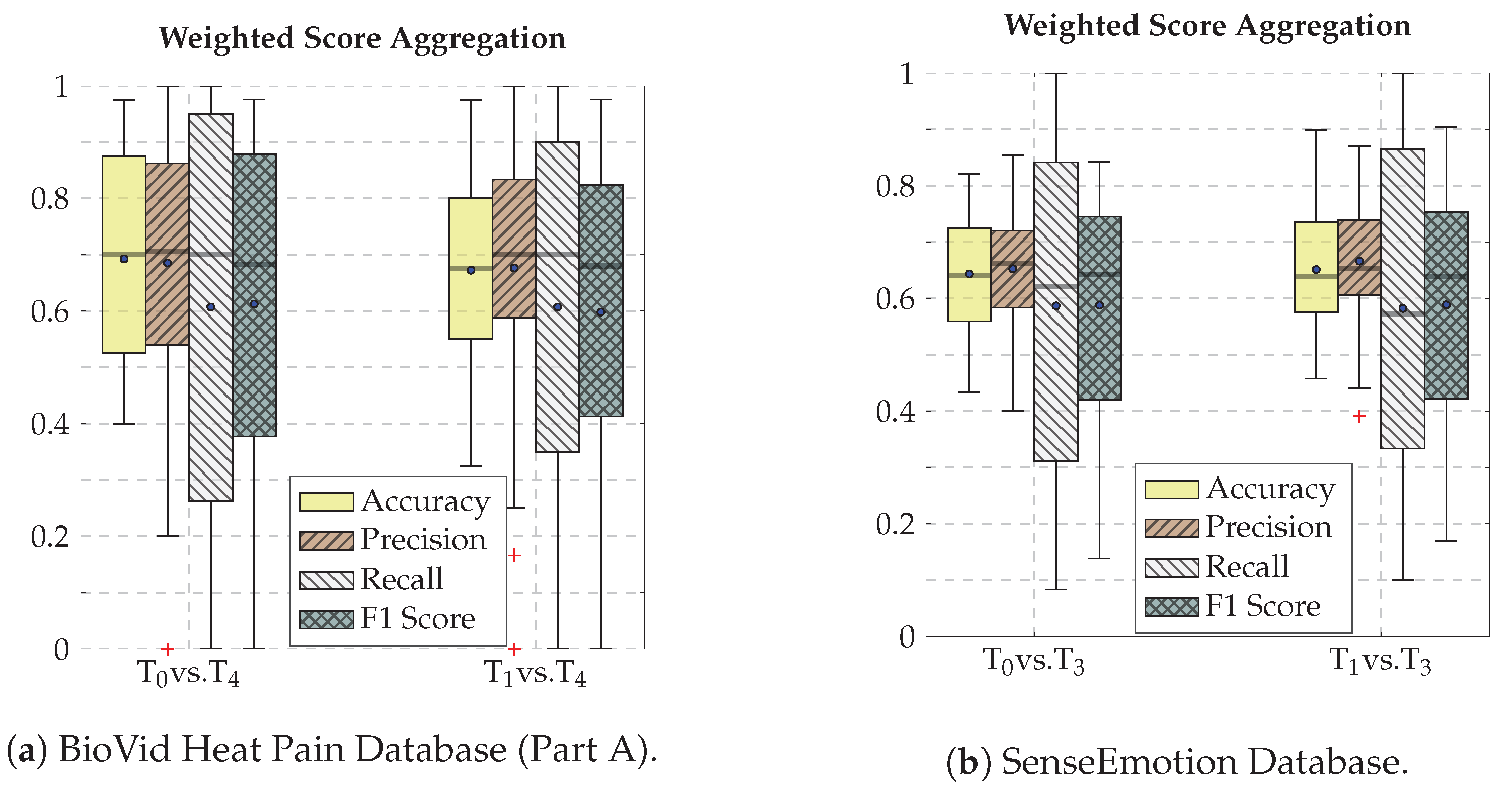
| Our Approach | Weighted Score Aggregation |
| Approach | Description | Performance |
|---|---|---|
| Kalischek et al. [38] | Transfer Learning | |
| Thiam et al. [15] | Standardised Geometric Features | |
| Our Approach | Motion Histogram Images | |
| Our Approach | Optical Flow Images | |
| Our Approach | Weighted Score Aggregation |
© 2020 by the authors. Licensee MDPI, Basel, Switzerland. This article is an open access article distributed under the terms and conditions of the Creative Commons Attribution (CC BY) license (http://creativecommons.org/licenses/by/4.0/).
Share and Cite
Thiam, P.; Kestler, H.A.; Schwenker, F. Two-Stream Attention Network for Pain Recognition from Video Sequences. Sensors 2020, 20, 839. https://doi.org/10.3390/s20030839
Thiam P, Kestler HA, Schwenker F. Two-Stream Attention Network for Pain Recognition from Video Sequences. Sensors. 2020; 20(3):839. https://doi.org/10.3390/s20030839
Chicago/Turabian StyleThiam, Patrick, Hans A. Kestler, and Friedhelm Schwenker. 2020. "Two-Stream Attention Network for Pain Recognition from Video Sequences" Sensors 20, no. 3: 839. https://doi.org/10.3390/s20030839