A Belief Network Reasoning Framework for Fault Localization in Communication Networks


Abstract
:1. Introduction
- We propose an overall framework to perform fault localization in communication networks, which allows for knowledge storage, inference, and message transmission.
- We apply PTNORgate to address the computational complexity problem. This helps to avoid the computational complexity in the calculation process of fault reasoning.
- We offer a solution for storing parameters in a network parameter table, such as a routing table in communication networks, with the aim of facilitating the development of the algorithm.
- The scheme that we offer carries out the reasoning process in an event-driven manner. This scheme improves the degree of automation of the localization process and reduces human intervention.
2. Related Works
3. Belief Networks as a Fault Propagation Method
3.1. The Definition and Notations of Belief Networks
3.2. The Noisy OR-Gate Model
4. Fault Localization Techniques
4.1. Messages Fuse and Propagate in Belief Networks
4.2. The Belief Update in Belief Networks
4.3. The Storage Mechanism of Belief Networks
4.4. Application of the Belief Propagation Algorithm to Fault Localization
- Fault nodes. If node X is a fault node, we set to be equal to its prior probability.
- Leaf nodes. Alarm node X is a node with no children. If X is instantiated, we set . In contrast, if X is in a normal state, we set . In addition, if X has only one parent, in order to prevent the parent from receiving , the message propagation between X and its one parent is restricted to . In other words, we assume that node U is the only parent of X, and the conditional probability between them is , if X is in a normal state, then , . In addition, if X is instantiated, , .
- Instantiated node. If node X is instantiated, we set , and regardless of the other values in the expression. Therefore, node X is turned into a leaf node, and the message propagation is a block between X and its children.
5. Case Study
6. Evaluation and Discussion
6.1. Evaluation Methodology
6.1.1. Generation of the Belief Network
6.1.2. Experiment Settings
6.2. Evaluation Result
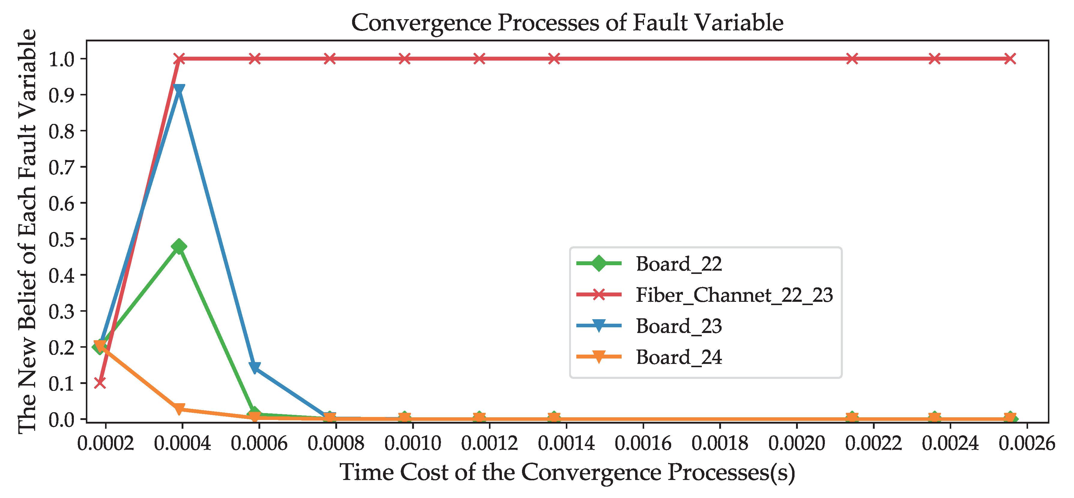
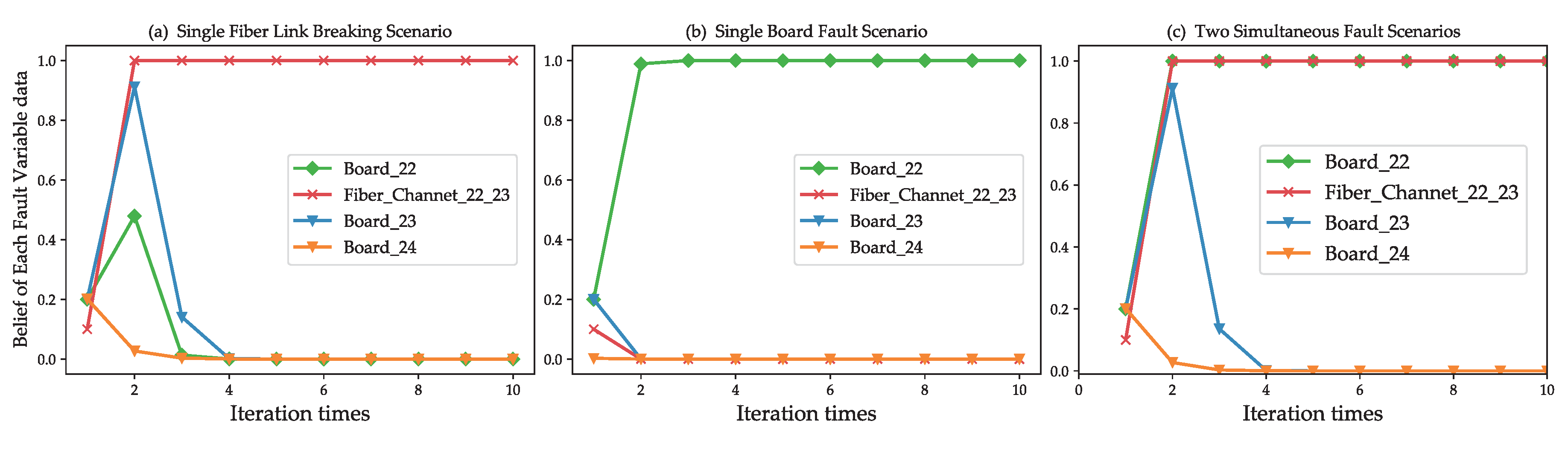
6.2.1. Convergence speed
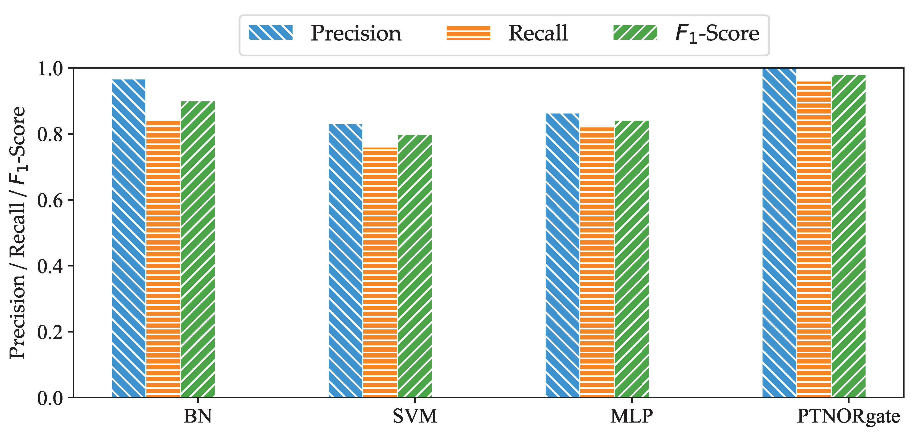
6.2.2. Reliability
- Precision: The ratio of the number of fault analysis reports correctly identified over the total number of fault analysis reports identifying faults. The higher the value of precision, the lower the misdiagnosis rate, and vice versa. The precision value can be computed as follows:where P is the precision value, is the number of true positives, and is the number of false positives.
- Recall: The ratio of the number of fault analysis reports correctly identified over the number of fault analysis reports that actually occurred. The higher the value of recall, the lower the misdiagnosis rate, and vice versa. The recall value is computed as follows:where is the number of false negatives.
- -: - is the harmonic average of the precision and recall. Higher the value of -, the better the performance of the approach. The - value can be computed as follows:
6.2.3. Capability to Deal with Multi Source Fault
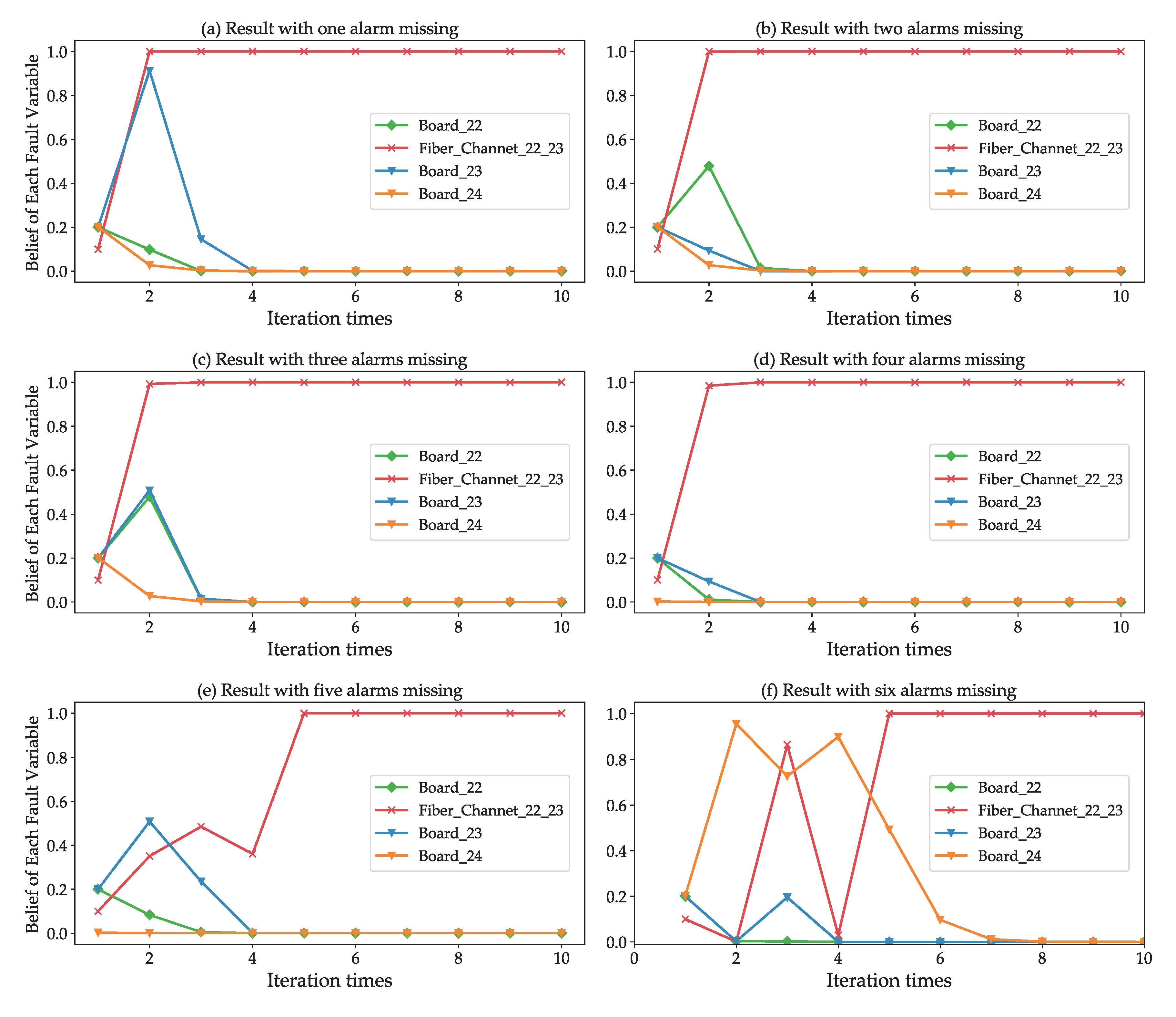
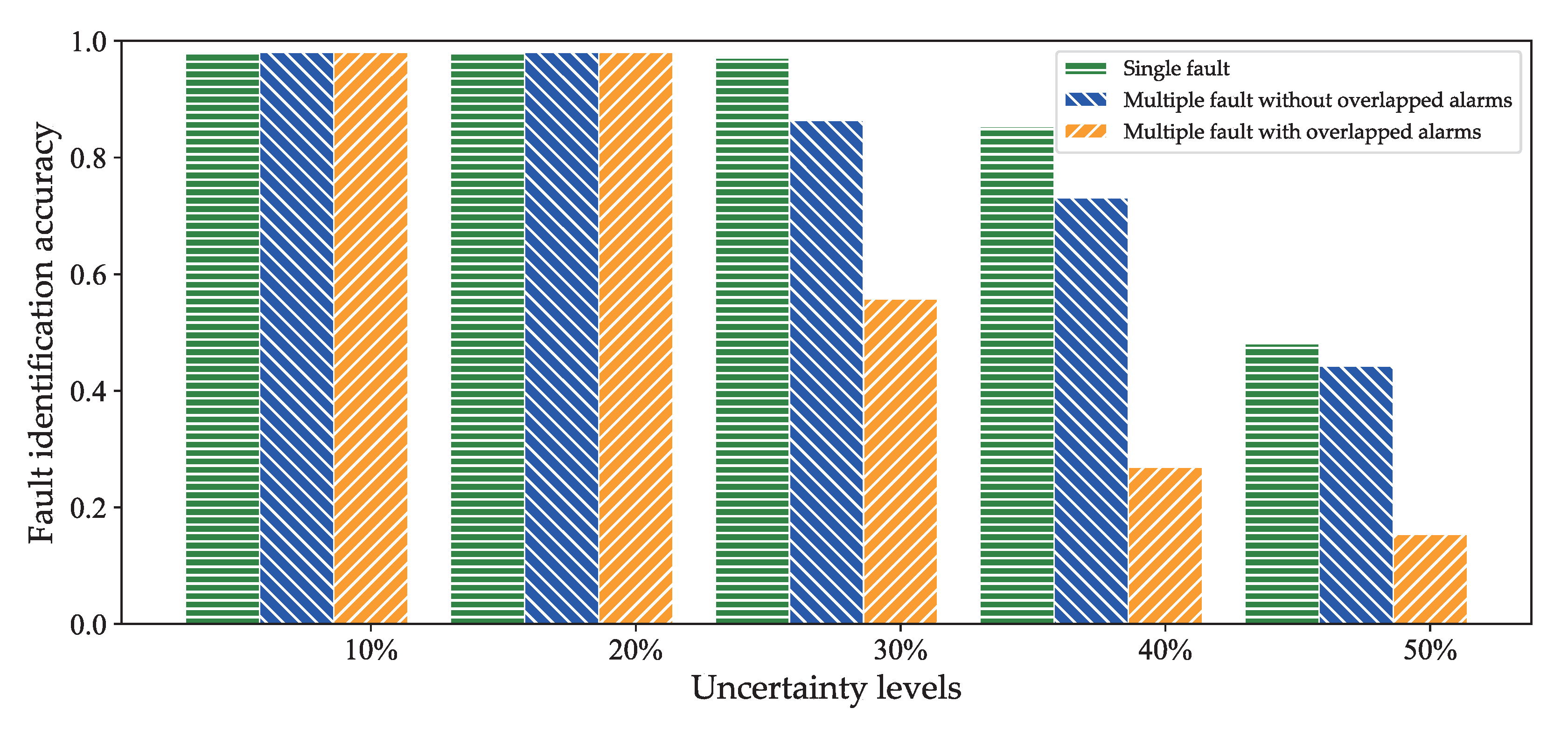
6.2.4. The Ability to Identify Faults in Uncertain Environments
7. Conclusions and Future Work
Author Contributions
Funding
Acknowledgments
Conflicts of Interest
References
- Yan, H.; Breslau, L.; Ge, Z.; Massey, D.; Pei, D.; Yates, J. G-RCA: A Generic Root Cause Analysis Platform for Service Quality Management in Large IP Networks. IEEE/ACM Trans. Netw. 2012, 20, 1734–1747. [Google Scholar] [CrossRef]
- Bennacer, L.; Amirat, Y.; Chibani, A.; Mellouk, A.; Ciavaglia, L. Self-Diagnosis Technique for Virtual Private Networks Combining Bayesian Networks and Case-Based Reasoning. IEEE Trans. Autom. Sci. Eng. 2014, 12, 354–366. [Google Scholar] [CrossRef]
- Ahmed, K.; Izadi, I.; Chen, T.; Joe, D.; Burton, T. Similarity analysis of industrial alarm flood data. IEEE Trans. Autom. Sci. Eng. 2013, 10, 452–457. [Google Scholar] [CrossRef]
- Cheng, Y.; Izadi, I.; Chen, T. Pattern matching of alarm flood sequences by a modified smith—Waterman algorithm. Chem. Eng. Res. Des. 2013, 91, 1085–1094. [Google Scholar] [CrossRef]
- Hu, W.; Wang, J.; Chen, T. A local alignment approach to similarity analysis of industrial alarm flood sequences. Control. Eng. Pract. 2016, 55, 13–25. [Google Scholar] [CrossRef]
- Dusia, A.; Sethi, A.S. Recent Advances in Fault Localization in Computer Networks. IEEE Commun. Surv. Tutor. 2016, 18, 3030–3051. [Google Scholar] [CrossRef]
- Jakobson, G.; Weissman, M. Alarm Correlation: Correlating Multiple Network Alarms Improves Telecommunications Network Surveillance and Fault Management. IEEE Netw. 1993, 7, 52–59. [Google Scholar] [CrossRef]
- Edmonds, M.; Kubricht, J.; Summers, C.; Zhu, Y.; Zhu, S.C. Human Causal Transfer: Challenges for Deep Reinforcement Learning. In Proceedings of the 40th Annual Meeting of the Cognitive Science Society, CogSci, Madison, WI, USA, 25–28 July 2018. [Google Scholar]
- Bengio, Y.; Deleu, T.; Rahaman, N.; Ke, R.; Lachapelle, S.; Bilaniuk, O.; Goyal, A.; Pal, C. A Meta-Transfer Objective for Learning to Disentangle Causal Mechanisms. arXiv 2019, arXiv:1901.10912v2. [Google Scholar]
- Pearl, J. Belief Updating by Network Propagation. In Probabilistic Reasoning in Intelligent Systems: Networks of Plausible Inference; Morgan Kaufmann Publisher: San Francisco, CA, USA, 1988; pp. 143–190. [Google Scholar]
- McCloghrie, K.; Rose, M. Management Information Base for Network Management of TCP/IP-Based Internets: MIB-II; RFC 1213; IETF Network Working Group, Hughes LAN System, Inc.: Germantown, MD, USA, 1991. [Google Scholar]
- Steinert, R.; Gillblad, D. Long-Term Adaptation and Distributed Detection of Local Network Changes. In Proceedings of the 2010 IEEE Global Telecommunications Conference GLOBECOM 2010, Miami, FL, USA, 6–10 December 2010; pp. 1–5. [Google Scholar]
- Díaz, S.; Escudero, J.I.; Luque, J. Expert System–Based Alarm Management In Communication Networks. In ICEIS; Secretariat, Escola Superior de Tecnologia de Set ú bal, Portugal: Stafford, UK, 2000; pp. 116–120. [Google Scholar]
- Cronk, R.; Callahan, P.; Bernstein, L. Rule-based expert systems for network management and operations: An introduction. IEEE Netw. 1988, 2, 7–21. [Google Scholar] [CrossRef]
- Klemettinen, M.; Mannila, H.; Toivonen, H. Rule discovery in telecommunication alarm data. J. Netw. Syst. Manag. 1999, 7, 395–423. [Google Scholar] [CrossRef]
- Wang, J.; He, C.; Liu, Y.; Tian, G.; Peng, I.; Xing, J.; Ruan, X.; Xie, H.; Wang, F.L. Efficient alarm behavior analytics for telecom networks. Inf. Sci. 2017, 402, 1–14. [Google Scholar] [CrossRef]
- Chen, Y.; Lee, J. Autonomous mining for alarm correlation patterns based on timeshift similarity clustering in manufacturing system. In Proceedings of the 2011 IEEE Conference on Prognostics and Health Management, Montreal, QC, Canada, 20–23 June 2011; pp. 1–8. [Google Scholar]
- Aamodt, A.; Plaza, E. Case-based reasoning: foundational issues, methodological variations, and system approaches. Ai Commun. 2001, 7, 39–59. [Google Scholar] [CrossRef]
- Silva, G.C.; Carvalho, E.E.; Caminhas, W.M. An artificial immune systems approach to Case-based Reasoning applied to fault detection and diagnosis. Expert Syst. Appl. 2020, 140, 112906. [Google Scholar] [CrossRef]
- Mohammed, M.A.; Ghani, M.K.A.; Arunkumar, N.; Obaid, O.I.; Mostafa, S.A.; Jaber, M.M.; Aboobaider, B.M.; Matar, B.M.; Abdullatif, S.K.; Ibrahim, D.A. Genetic case-based reasoning for improved mobile phone faults diagnosis. Comput. Electr. Eng. 2018, 71, 212–222. [Google Scholar] [CrossRef]
- Srinivasan, S.M.; Truong-Huu, T.; Gurusamy, M. Machine Learning-Based Link Fault Identification and Localization in Complex Networks. IEEE Internet Things J. 2019, 6, 6556–6566. [Google Scholar] [CrossRef] [Green Version]
- Wang, M.; Cui, Y.; Wang, X.; Xiao, S.; Jiang, J. Machine Learning for Networking: Workflow, Advances and Opportunities. IEEE Netw. 2018, 32, 92–99. [Google Scholar] [CrossRef] [Green Version]
- Ferreira, V.C.; Carrano, R.; Silva, J.O.; Albuquerque, C.; Muchaluat-Saade, D.C.; Passos, D. Fault Detection and Diagnosis for Solar-powered Wireless Mesh Networks using Machine Learning. In Proceedings of the IFIP/IEEE IM 2017, Lisbon, Portugal, 8–12 May 2017; pp. 456–462. [Google Scholar]
- Cheng, M.X.; Wu, W.B. Data Analytics for Fault Localization in Complex Networks. IEEE Internet Things 2016, 3, 701–708. [Google Scholar] [CrossRef]
- Zidi, S.; Moulahi, T.; Alaya, B. Fault Detection in Wireless Sensor Networks Through SVM Classifier. IEEE Sens. J. 2018, 18, 340–347. [Google Scholar] [CrossRef]
- Khunteta, S.; Chavva, A.K.R. Deep Learning Based Link Failure Mitigation. In Proceedings of the 2017 16th IEEE International Conference on Machine Learning and Applications (ICMLA), Cancun, Mexico, 18–21 December 2017; pp. 806–811. [Google Scholar]
- Yongli, Z.; Limin, H.; Jinling, L. Bayesian networks-based approach for power systems fault diagnosis. IEEE Trans. Power Deliv. 2006, 21, 634–639. [Google Scholar] [CrossRef]
- Amjad, M.; Nabil, A.; Mithun, M.; Salwani, A.; Houbing, S. A survey on proactive, active and passive fault diagnosis protocols for wsns: network operation perspective. Sensors 2018, 18, 1787. [Google Scholar]
- Steinder, M.; Sethi, A.S. Probabilistic fault localization in communication systems using belief networks. IEEE ACM Trans. Netw. 2004, 12, 809–822. [Google Scholar] [CrossRef]
- Dong, L.; Wesseloo, J.; Potvin, Y.; Li, X. Discrimination of Mine Seismic Events and Blasts Using the Fisher Classifier, Naive Bayesian Classifier and Logistic Regression. Rock Mech. Rock Eng. 2016, 49, 183–211. [Google Scholar] [CrossRef]
- Dong, L.; Li, X.; Xie, G. Nonlinear Methodologies for Identifying Seismic Event and Nuclear Explosion Using Random Forest, Support Vector Machine, and Naive Bayes Classification. Abstr. Appl. Anal. 2014, 2014, 1–8. [Google Scholar] [CrossRef] [Green Version]
- Narendrasinh, B.G.; Vdevyas, D. Fuzzy lion Bayes system for intrusion detection in wireless communication network. J. Cent. South Univ. 2019, 26, 3017–3033. [Google Scholar] [CrossRef]
- Jun, H.; Kim, D.S. A Bayesian network-based approach for fault analysis. Expert Syst. Appl. 2017, 81, 332–348. [Google Scholar] [CrossRef]
- Huang, Y.; Wang, Y.; Zhang, R. Fault Troubleshooting Using Bayesian Network and Multicriteria Decision Analysis . Adv. Mech. Eng. 2014, 6, 282013. [Google Scholar]
- Wang, J.; Wang, Z.; Stetsyuk, V.; Ma, X.; Gu, F.; Li, W. Exploiting Bayesian networks for fault isolation: A diagnostic case study of diesel fuel injection system. Isa Trans. 2019, 86, 276–286. [Google Scholar] [CrossRef] [Green Version]
- Yoon, S. In-situ sensor calibration in an operational air-handling unit coupling autoencoder and Bayesian inference. Energy Build. 2020, 221, 110026. [Google Scholar] [CrossRef]
- Zheng, T.; Xiaoguang, G. Research on the self-defence electronic jamming decision-making based on the discrete dynamic Bayesian network. J. Syst. Eng. Electron. 2008, 19, 702–708. [Google Scholar] [CrossRef]
- Wang, J.; Yang, Z.; Su, J.; Zhao, Y.; Gao, S.; Pang, X.; Zhou, D. Root-cause analysis of occurring alarms in thermal power plants based on Bayesian networks. Int. J. Electr. Power Energy Syst. 2018, 103, 67–74. [Google Scholar] [CrossRef]
- Hossain, N.U.I.; Jaradat, R.; Hosseini, S.; Marufuzzaman, M.; Buchanan, R.K. A framework for modeling and assessing system resilience using a bayesian network: A case study of an interdependent electrical infrastructure system. Int. J. Crit. Infrastruct. Prot. 2019, 25, 62–83. [Google Scholar] [CrossRef]
- Yu, J.; Rashid, M. A novel dynamic bayesian network-based networked process monitoring approach for fault detection, propagation identification, and root cause diagnosis. Aiche J. 2013, 59, 2348–2365. [Google Scholar] [CrossRef]
- Yu, J.; Rashid, M.M. Dynamic process fault detection and diagnosis based on a combined approach of hidden Markov and Bayesian network model. Chem. Eng. Sci. 2019, 59, 82–96. [Google Scholar]
- Zhao, Y.; Tong, J.; Zhang, L.; Wu, G. Diagnosis of operational failures and on-demand failures in nuclear power plants: An approach based on dynamic bayesian networks. Ann. Nucl. Energy 2020, 138, 107181. [Google Scholar] [CrossRef]
- Guohua, W.; Jiejuan, T.; Liguo, Z.; Yunfei, Z.; Zhiyong, D. Framework for fault diagnosis with multi-source sensor nodes in nuclear power plants based on a bayesian network. Ann. Nucl. Energy 2018, 122, 297–308. [Google Scholar]
- Oniśko, A.; Druzdzel, M.J. Impact of precision of Bayesian network parameters on accuracy of medical diagnostic systems. Artif. Intell. Med. 2013, 57, 197–206. [Google Scholar] [CrossRef] [Green Version]
- Arias, J.; Martinezgomez, J.; Gamez, J.A.; De Herrera, A.G.; Muller, H. Medical image modality classification using discrete Bayesian networks. Comput. Vis. Image Underst. 2016, 151, 61–71. [Google Scholar] [CrossRef] [Green Version]
- Li, M.; Liu, Z.; Li, X.; Liu, Y.; Mei, L.; Zixian, L.; Xiaopeng, L.; Yiliu, L. Dynamic risk assessment in healthcare based on Bayesian approach. Reliab. Eng. Syst. Saf. 2019, 189, 327–334. [Google Scholar] [CrossRef]
- Jensen, F.V.; Nielsen, T.D. Causal and Bayesian Networks. In Bayesian Networks and Decision Graphs, 2nd ed.; Jordan, M., Kleinberg, J., Schölkopf, B., Eds.; Springer: New York, NY, USA, 2007; pp. 44–45. [Google Scholar]
- Steinder, M.; Sethi, A. End-to-end Service Failure Diagnosis Using Belief Networks. In Proceedings of the NOMS 2002, IEEE/IFIP Network Operations and Management Symposium, ’Management Solutions for the New Communications World’ (Cat. No.02CH37327), Florence, Italy, 19 April 2002. [Google Scholar]
- Zhang, P.; Shu, S.; Zhou, M. An Online Fault Detection Model and Strategies Based on SVM-grid in Clouds. IEEE/CAA J. Autom. Sin. 2018, 5, 445–456. [Google Scholar] [CrossRef]
- Gardner, M.W.; Dorling, S.R. Artificial Neural Networks (the Multilayer Perceptron)—A Review of Applications in the Atmospheric Sciences. Atmos. Environ. 1998, 32, 2627–2636. [Google Scholar] [CrossRef]


| Relationship | Name | Prior Probability | Belief | ||||
|---|---|---|---|---|---|---|---|
| Self | X | ||||||
| father | |||||||
| father | |||||||
| ⋮ | ⋮ | ⋮ | ⋮ | ||||
| father | |||||||
| child | |||||||
| child | |||||||
| ⋮ | ⋮ | ⋮ | ⋮ | ||||
| child |
| Variable | Fault 1 | Fault 2 | Fault 3 | Alarm 1 | Alarm 2 | Alarm 3 | Alarm 4 | Alarm 5 |
|---|---|---|---|---|---|---|---|---|
| Value | (0.1418, | (0.1882, | (0.9346, | (0.16, | (0.9078, | (1,0) | (1,0) | (1,0) |
| 0.8582) | 0.8118) | 0.0654) | 0.84) | 0.0922) |
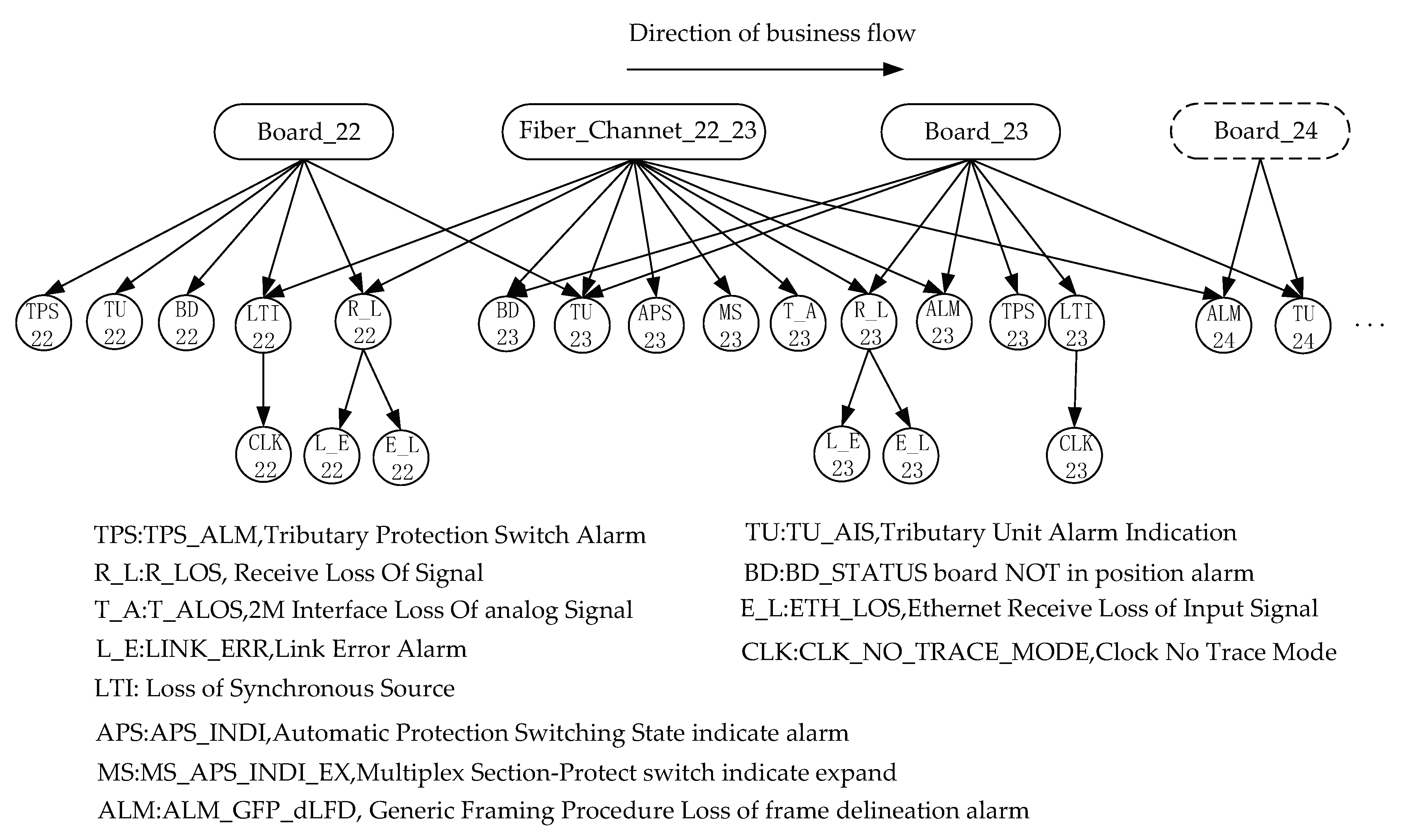
| Sites | NE-22 | NE-23 | NE-24 |
|---|---|---|---|
| Alarm | R-L, LTI, CLK | BD, TU, APS, MS, T-A, R-L, ALM, E-L | ALM |
| Number of Nodes | 100 | 200 | 400 | 600 | 800 | 1000 | 2000 |
|---|---|---|---|---|---|---|---|
| 0.0005 | 0.0010 | 0.0020 | 0.0028 | 0.0042 | 0.0053 | 0.0097 | |
| 0.0006 | 0.0010 | 0.0026 | 0.0038 | 0.0042 | 0.0050 | 0.0094 | |
| 0.0006 | 0.0011 | 0.0020 | 0.0028 | 0.0040 | 0.0050 | 0.0097 | |
| 0.0006 | 0.0010 | 0.0020 | 0.0035 | 0.0041 | 0.0053 | 0.0101 | |
| Time per iteration (s) | 0.0007 | 0.0010 | 0.0020 | 0.0029 | 0.0043 | 0.0054 | 0.0097 |
| 0.0006 | 0.0010 | 0.0022 | 0.0034 | 0.0041 | 0.0050 | 0.0093 | |
| 0.0006 | 0.0010 | 0.0020 | 0.0029 | 0.0045 | 0.0051 | 0.0094 | |
| 0.0006 | 0.0010 | 0.0020 | 0.0033 | 0.0040 | 0.0053 | 0.0096 | |
| 0.0006 | 0.0010 | 0.0023 | 0.0030 | 0.0051 | 0.0053 | 0.0099 | |
| Time to reach equilibrium (s) | 0.0054 | 0.0091 | 0.0191 | 0.0284 | 0.0385 | 0.0467 | 0.0868 |
| Localization Methods | Time Required for 2000 Nodes (s) | |
|---|---|---|
| Traditional Bayesian network (BN) | 6.3207 | |
| Support vector machine (SVM) | 2.0763 | |
| Multi-layer perceptron (MLP) | 0.2498 | |
| Polytrees with noisy OR-gate (PTNORgate) | 0.0868 |
Publisher’s Note: MDPI stays neutral with regard to jurisdictional claims in published maps and institutional affiliations. |
© 2020 by the authors. Licensee MDPI, Basel, Switzerland. This article is an open access article distributed under the terms and conditions of the Creative Commons Attribution (CC BY) license (http://creativecommons.org/licenses/by/4.0/).
Share and Cite
Liang, R.; Liu, F.; Liu, J. A Belief Network Reasoning Framework for Fault Localization in Communication Networks. Sensors 2020, 20, 6950. https://doi.org/10.3390/s20236950
Liang R, Liu F, Liu J. A Belief Network Reasoning Framework for Fault Localization in Communication Networks. Sensors. 2020; 20(23):6950. https://doi.org/10.3390/s20236950
Chicago/Turabian StyleLiang, Rongyu, Feng Liu, and Jie Liu. 2020. "A Belief Network Reasoning Framework for Fault Localization in Communication Networks" Sensors 20, no. 23: 6950. https://doi.org/10.3390/s20236950