Flow Control Based on Feature Extraction in Continuous Casting Process


Abstract
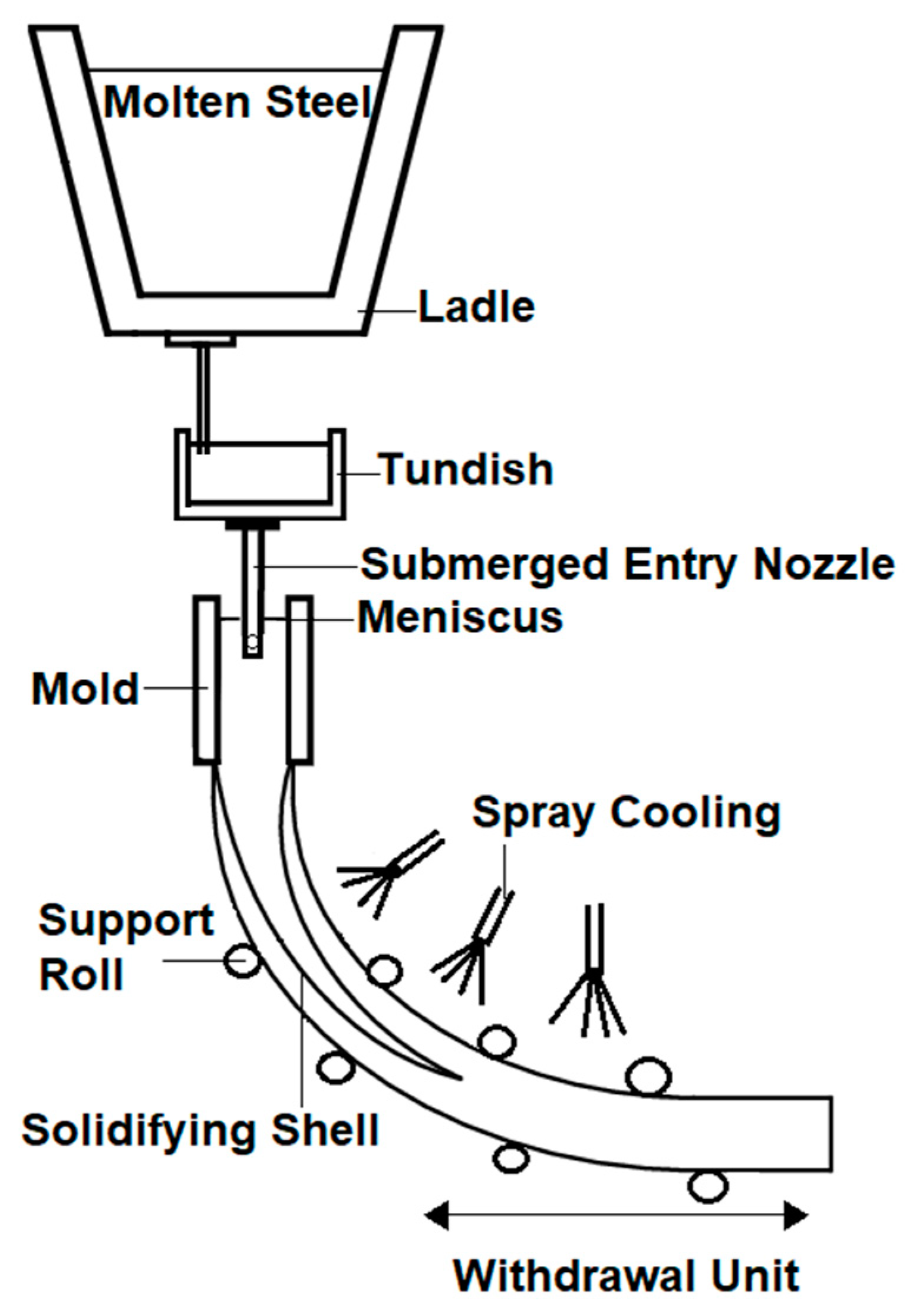
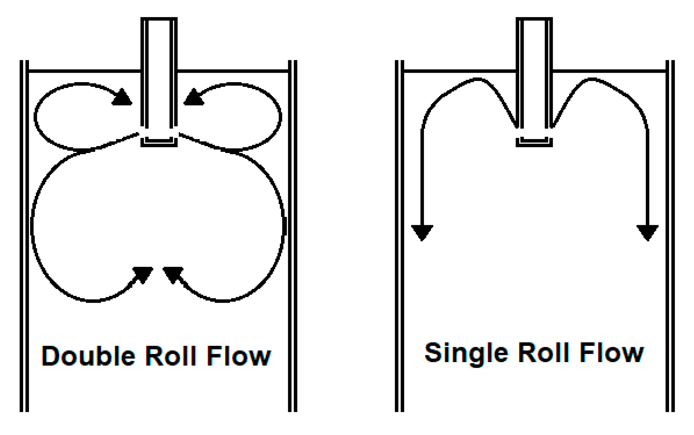
:1. Introduction
2. Experimental Setup
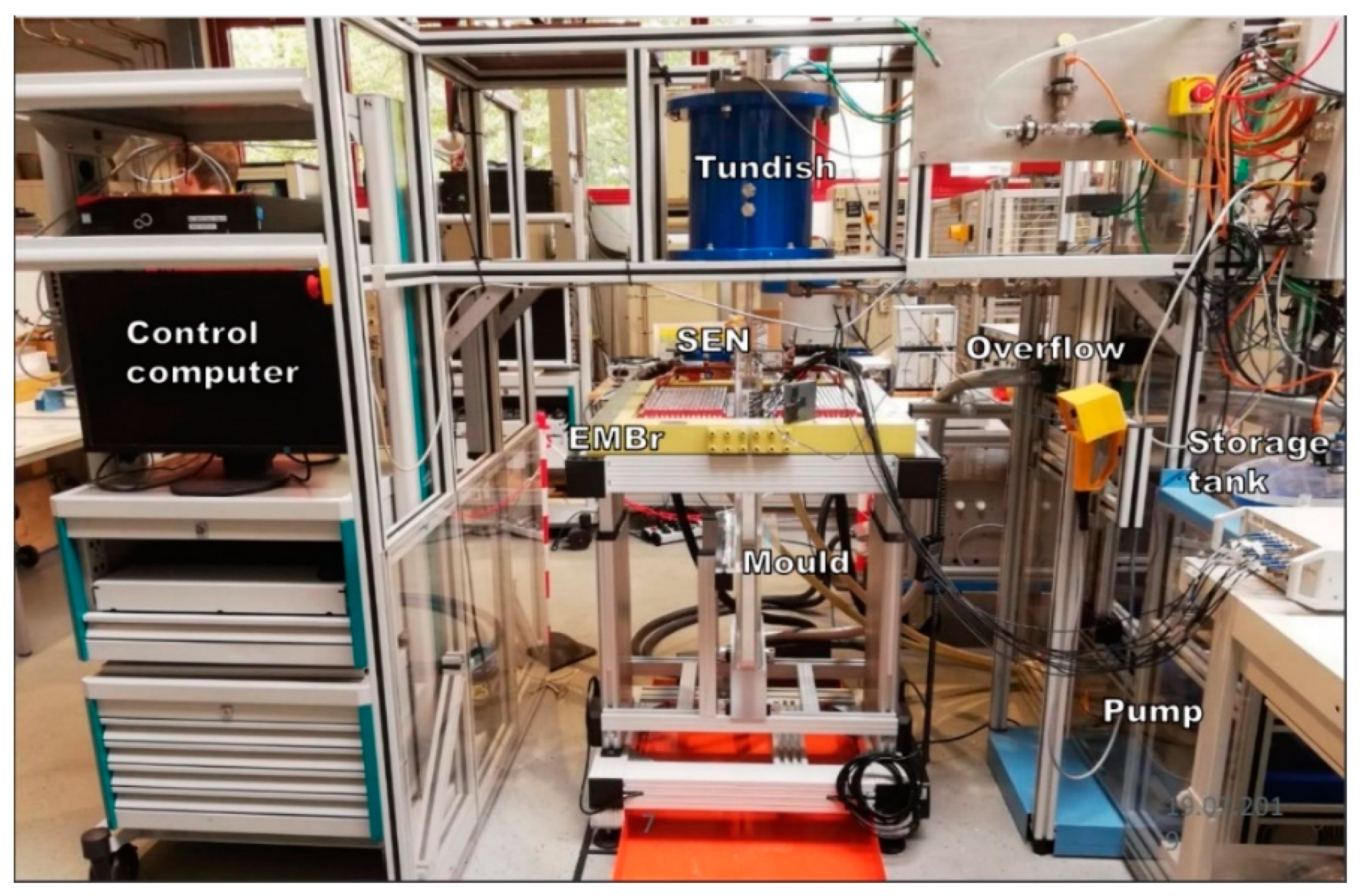
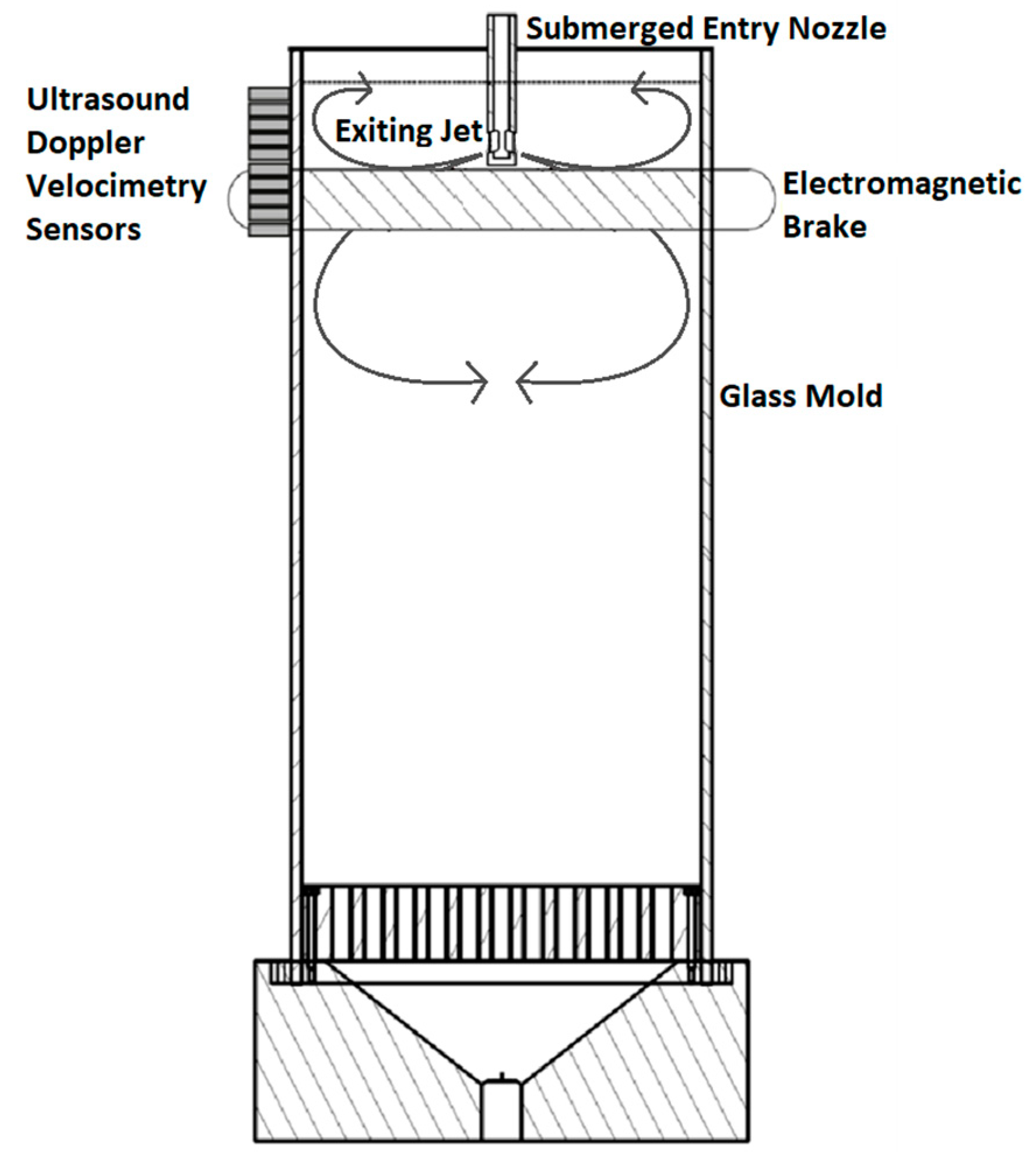
2.1. Mini-LIMMCAST Facility
2.2. Electromagnetic Brake
3. Pre-Processing Data for Control
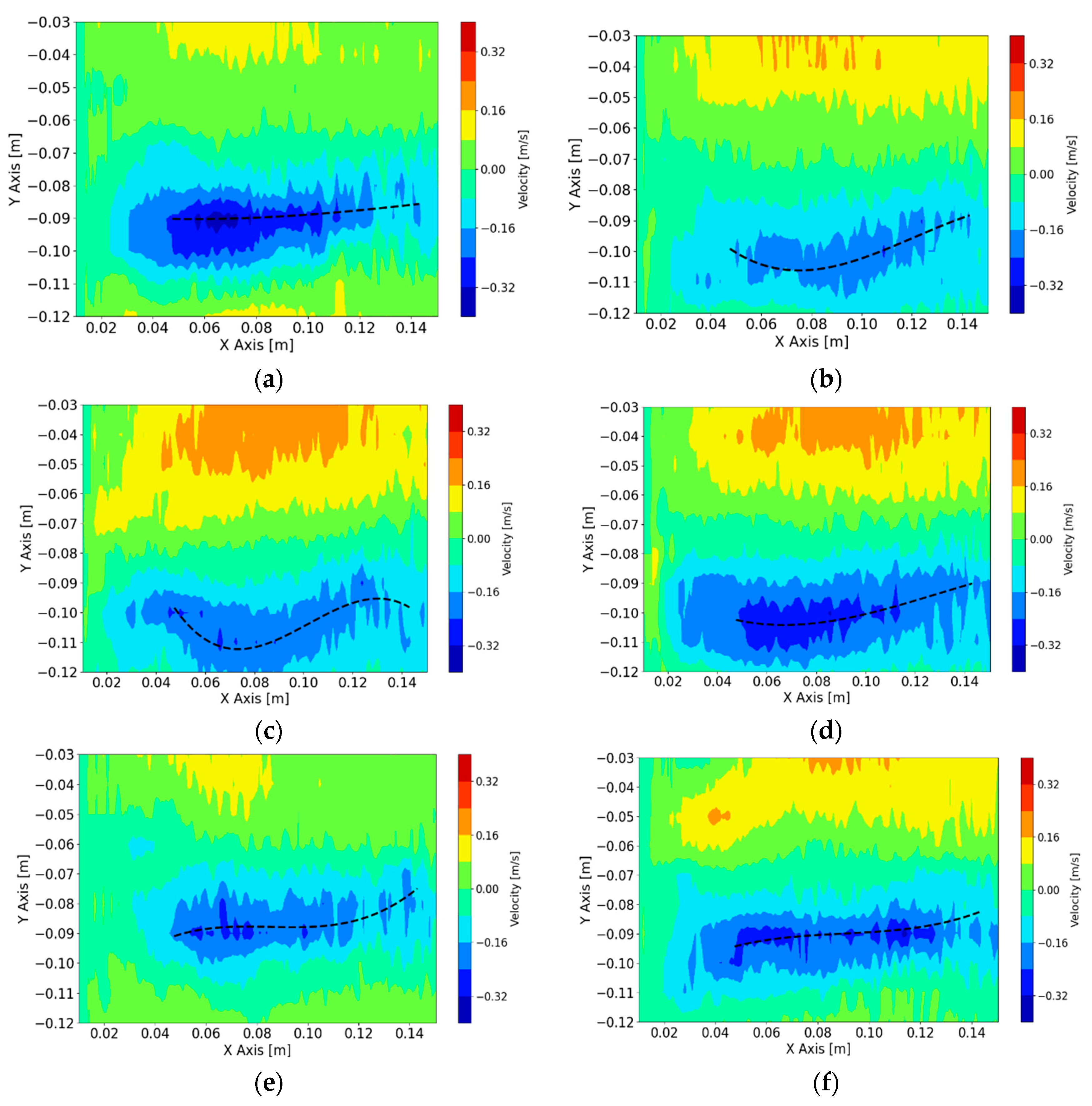
3.1. Pre-Processing of the UDV Data
3.2. Feature Extraction
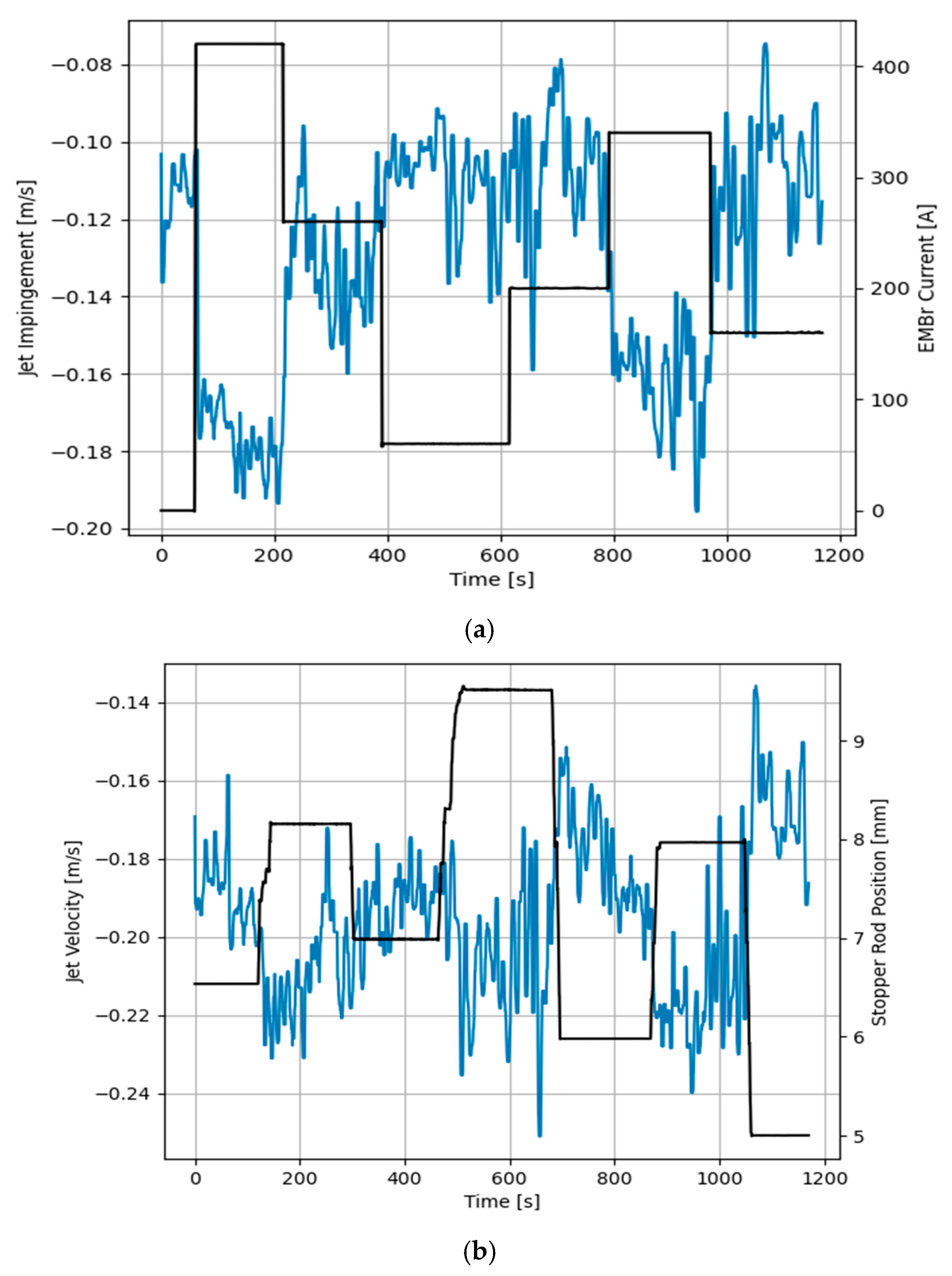
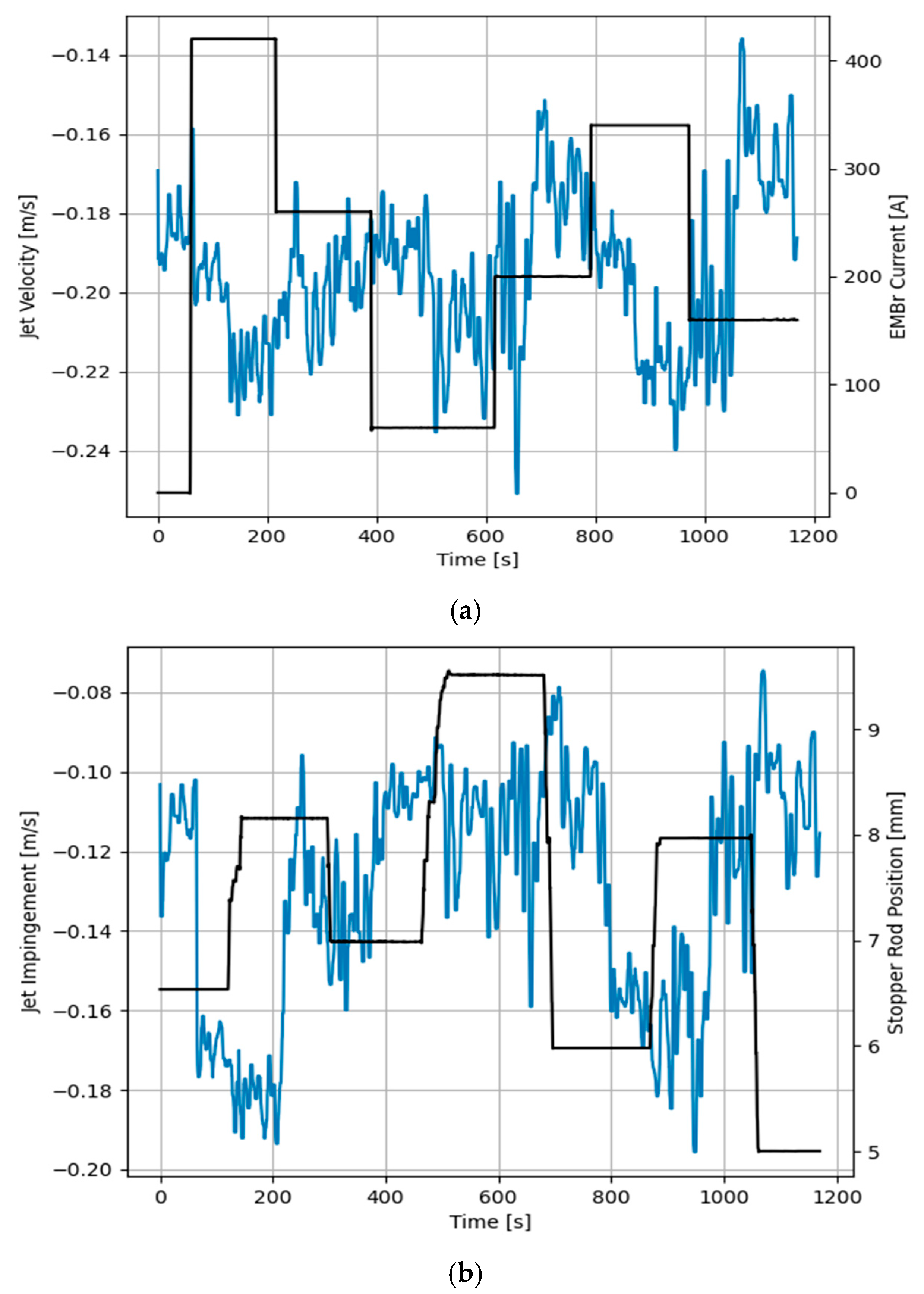
3.3. System Identification
4. Model Predictive Control
5. Results and Discussion
6. Conclusions
- (1)
- We can avoid using the entire velocity map measured by the UDV by quantifying specific features from the raw data. This allows for less processing time for the controller and allows for conventional control techniques to be applied as the distributed parameter system is simplified to a lumped parameter system.
- (2)
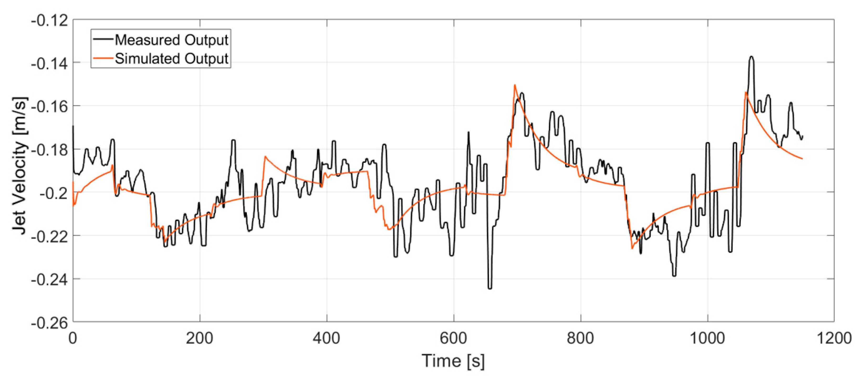
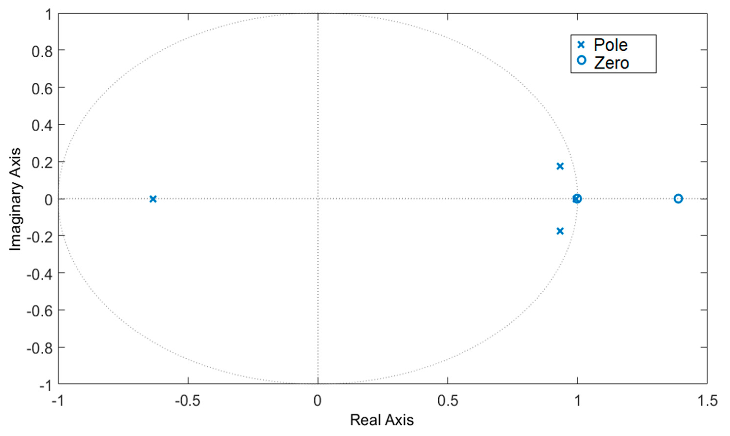
- The deterministic part of the relationship between the manipulated variables (current of the electromagnetic brake and position of the stopper rod) and the controlled variables (jet impingement point and jet velocity) can be described by a model obtained using system identification methods. Measurement data from the experimental setup is used for this process. In the end, a 4th order discrete state space model with two inputs and two outputs can capture the essential dynamics of the relationship between manipulated and controlled variables.
- (3)
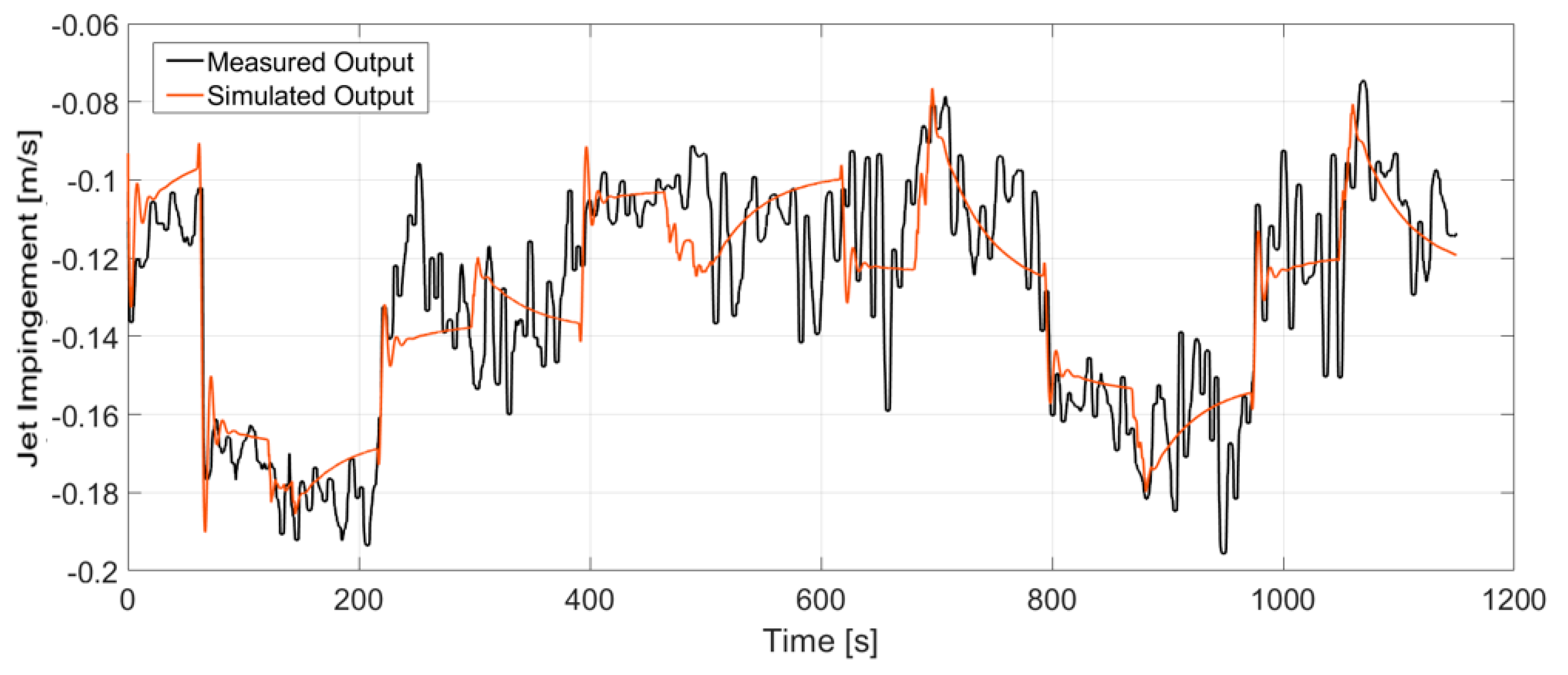
- This black-box model created by using system identification is able to describe the dynamic responses of the system, however it should be taken into consideration that the stochastic effect of turbulent flow is not described by the model.
- (4)
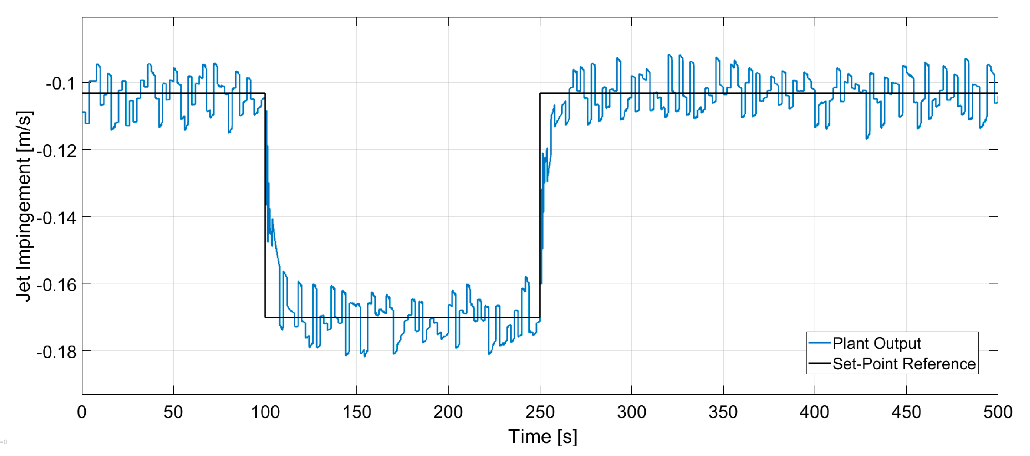
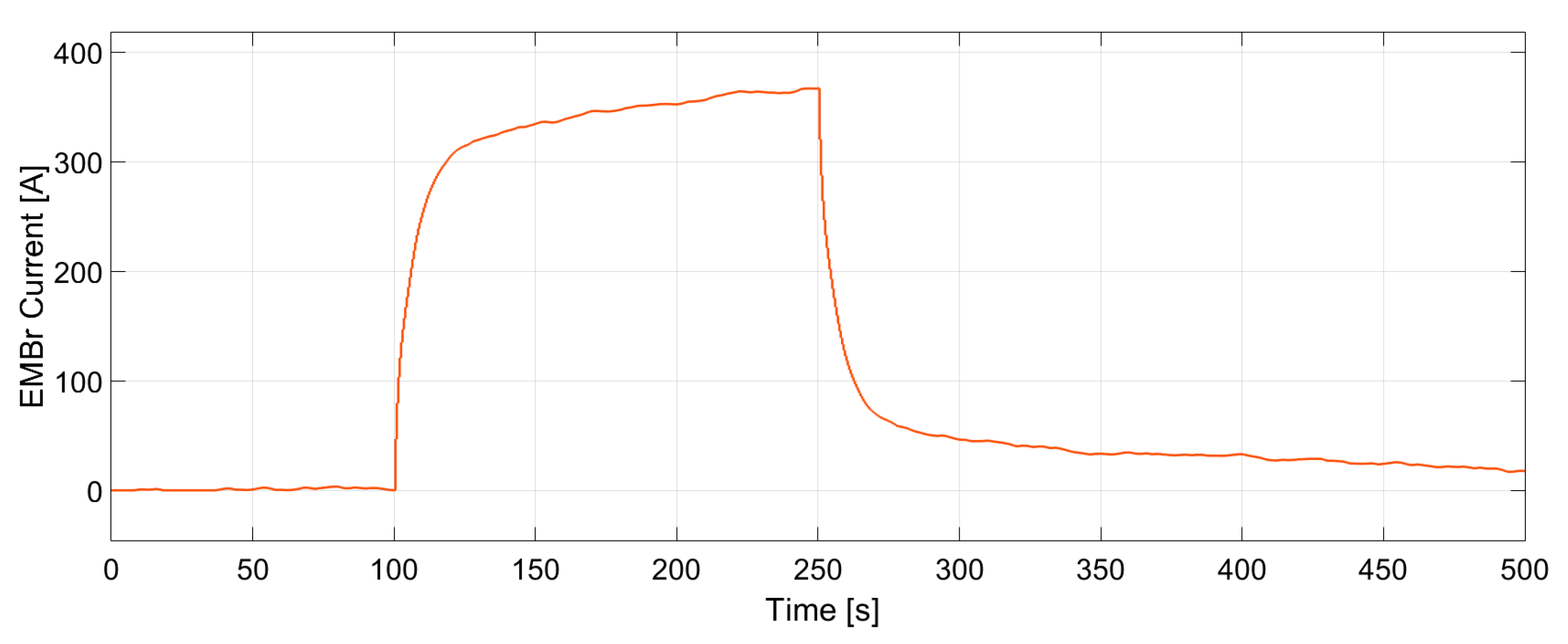
- The model is precise enough to be used as a part of the model based predictive controller. The control technique allows the constraints on the manipulated variables to be taken into account while designing the algorithm for the controller. The controller is able to track both set-points without exceeding any constraints. In this way optimal flow structures in the mold can be achieved.
Author Contributions
Funding
Conflicts of Interest
Abbreviations
| EMBr | Electromagnetic Brake |
| GaInSn | Gallium-Indium-Tin |
| UDV | Ultrasound Doppler Velocimetry |
| MPC | Model Predictive Control |
| SEN | Submerged Entry Nozzle |
| ECT | Electrical Capacitance Tomography |
References
- Thomas, B.G. On-Line Detection of Quality Problems in Continuous Casting of Steel. In Modeling, Control and Optimization in Ferrous and Nonferrous Industry, 2003 Materials Science & Technology Symposium; TMS: Warrendale, PA, USA, 2003; p. 16. [Google Scholar]
- Thomas, B.G. Review on Modeling and Simulation of Continuous Casting. Steel Res. Int. 2018, 89, 1700312. [Google Scholar] [CrossRef]
- Kim, M.; Moon, S.; Na, C.; Lee, D.; Kueon, Y.; Lee, J.S. Control of Mold Level in Continuous Casting Based on a Disturbance Observer. J. Process Control 2011, 21, 1022–1029. [Google Scholar] [CrossRef]
- Furtmueller, C.; del Re, L. Control Issues in Continuous Casting of Steel. IFAC Proc. Vol. 2008, 41, 700–705. [Google Scholar] [CrossRef] [Green Version]
- Thomas, B.G.; Cho, S.M. Overview of Electromagnetic Forces to Control Flow During Continuous Casting of Steel. IOP Conf. Ser. Mater. Sci. Eng. 2018, 424, 012027. [Google Scholar] [CrossRef]
- Kunstreich, S.; Dauby, P.H. Effect of Liquid Steel Flow Pattern on Slab Quality and the Need for Dynamic Electromagnetic Control in the Mould. Ironmak. Steelmak. 2005, 32, 80–86. [Google Scholar] [CrossRef]
- Cho, S.-M.; Thomas, B.G. Electromagnetic Forces in Continuous Casting of Steel Slabs. Metals 2019, 9, 471. [Google Scholar] [CrossRef] [Green Version]
- Cukierski, K.; Thomas, B.G. Flow Control with Local Electromagnetic Braking in Continuous Casting of Steel Slabs. Metall. Mater. Trans. B 2008, 39, 94–107. [Google Scholar] [CrossRef]
- Maurya, A.; Jha, P.K. Influence of Electromagnetic Stirrer Position on Fluid Flow and Solidification in Continuous Casting Mold. Appl. Math. Model. 2017, 48, 736–748. [Google Scholar] [CrossRef]
- Zhang, L.; Thomas, B.G. State of the Art in Evaluation and Control of Steel Cleanliness. ISIJ Int. 2003, 43, 271–291. [Google Scholar] [CrossRef] [Green Version]
- Zhang, T.; Yang, J.; Jiang, P. Measurement of Molten Steel Velocity near the Surface and Modeling for Transient Fluid Flow in the Continuous Casting Mold. Metals 2019, 9, 36. [Google Scholar] [CrossRef] [Green Version]
- Hashimoto, Y.; Matsui, A.; Hayase, T.; Kano, M. Real-time estimation of molten steel flow in continuous casting mold. Metall. Mater. Trans. B 2020, 51, 581–588. [Google Scholar] [CrossRef]
- Sedén, M.; Jacobson, N. Online Flow Control with Mold Flow Measurements and Simultaneous Braking and Stirring. IOP Conf. Ser. Mater. Sci. Eng. 2018, 424, 012015. [Google Scholar] [CrossRef] [Green Version]
- Choi, Y.J.; Mccarthy, K.L.; Mccarthy, M.J. Tomographic Techniques for Measuring Fluid Flow Properties. J. Food Sci. 2002, 67, 2718–2724. [Google Scholar] [CrossRef]
- Abouelazayem, S.; Glavinić, I.; Wondrak, T.; Hlava, J. Control of Jet Flow Angle in Continuous Casting Process Using an Electromagnetic Brake. IFAC-PapersOnLine 2019, 52, 88–93. [Google Scholar] [CrossRef]
- Abouelazayem, S.; Glavinić, I.; Wondrak, T.; Hlava, J. Adaptive Control of Meniscus Velocity in Continuous Caster Based on NARX Neural Network Model. IFAC-PapersOnLine 2019, 52, 222–227. [Google Scholar] [CrossRef]
- Schurmann, D.; Glavinić, I.; Willers, B.; Timmel, K.; Eckert, S. Impact of the Electromagnetic Brake Position on the Flow Structure in a Slab Continuous Casting Mold: An Experimental Parameter Study. Metall. Mater. Trans. B 2020, 51, 61–78. [Google Scholar] [CrossRef]
- Dekemele, K.; Ionescu, C.-M.; De Doncker, M.; De Keyser, R. Closed Loop Control of an Electromagnetic Stirrer in the Continuous Casting Process. In Proceedings of the 2016 European Control Conference (ECC), Aalborg, Denmark, 29 June–1 July 2016; pp. 61–66. [Google Scholar]
- Vakhrushev, A.; Liu, Z.Q.; Wu, M.H.; Kharicha, A.; Ludwig, A.; Nitzl, G.; Tang, T.; Hackl, G. Numerical modeling of the MHD flow in continuous casting mold by two CFD platforms ANSYS Fluent and OpenFOAM. In Proceedings of the 7th International Congress on Science and Technology of Steelmaking, Venice, Italy, 13–15 June 2018. [Google Scholar]
- Xie, D.; Huang, Z.; Ji, H.; Li, H. An Online Flow Pattern Identification System for Gas–Oil Two-Phase Flow Using Electrical Capacitance Tomography. IEEE Trans. Instrum. Meas. 2006, 55, 1833–1838. [Google Scholar] [CrossRef]
- Bukhari, S.F.A.; Yang, W.; McCann, H. A Hybrid Control Strategy for Oil Separators Based on Electrical Capacitance Tomography Images. Meas. Control 2007, 40, 211–217. [Google Scholar] [CrossRef]
- Zhang, L.; Yang, S.; Cai, K.; Li, J.; Wan, X.; Thomas, B.G. Investigation of Fluid Flow and Steel Cleanliness in the Continuous Casting Strand. Metall. Mater. Trans. B 2007, 38, 63–83. [Google Scholar] [CrossRef]
- Thomas, B.G. Chapter 15 in Modeling for Casting and Solidification Processing; Yu, O., Ed.; Marcel Dekker: New York, NY, USA, 2001; pp. 499–540. [Google Scholar]
- Thomas, B.G. Modeling of the Continuous Casting of Steel—Past, Present, and Future. Metall. Mater. Trans. B 2002, 33, 795–812. [Google Scholar] [CrossRef]
- Tanaskovic, M.; Fagiano, L.; Gligorovski, V. Adaptive Model Predictive Control for Linear Time Varying MIMO Systems. Automatica 2019, 105, 237–245. [Google Scholar] [CrossRef] [Green Version]
- Wiese, A.P.; Blom, M.J.; Manzie, C.; Brear, M.J.; Kitchener, A. Model Reduction and MIMO Model Predictive Control of Gas Turbine Systems. Control Eng. Pract. 2015, 45, 194–206. [Google Scholar] [CrossRef]
- Soliman, M.; Malik, O.P.; Westwick, D.T. Multiple Model MIMO Predictive Control for Variable Speed Variable Pitch Wind Turbines. In Proceedings of the 2010 American Control Conference, Baltimore, MD, USA, 30 June–2 July 2010; IEEE: Piscataway, NJ, USA, 2010. [Google Scholar]
- Get Started with Model Predictive Control Toolbox. Available online: https://www.mathworks.com/help/mpc/ug/optimization-problem.html (accessed on 22 October 2020).
- Ratajczak, M.; Wondrak, T.; Stefani, F. A gradiometric version of contactless inductive flow tomography: Theory and first applications. Philos. Trans. R. Soc. A Math. Phys. Eng. Sci. 2016, 374, 20150330. [Google Scholar] [CrossRef] [PubMed] [Green Version]


| Values | |
|---|---|
| Reference Temperature (°C) | 20 |
| Density () | 6353 |
| Kinematic Viscosity () | 3.44 × 10⁻⁷ |
| Electrical Conductivity () | 3.29 × 10⁻⁷ |
| Thermal Conductivity () | 23.98 |
| Surface Tension | 0.587 |
| Dimensions | |
|---|---|
| Mold Width (mm) | 300 |
| Mold Thickness (mm) | 35 |
| Mold Height (mm) | 600 |
| Submerged Entry Nozzle Immersion Depth (mm) | 35 ± 10 |
| Submerged Entry Nozzle Inner Diameter (mm) | 12 |
| Submerged Entry Nozzle Outer Diameter (mm) | 21 |
| Submerged Entry Nozzle Port Width (mm) | 11 |
| Submerged Entry Nozzle Port Height (mm) | 13 |
| Submerged Entry Nozzle Port Angle (deg) | −15 |
| Electromagnetic Brake Windings per Coil | 32 |
| Electromagnetic Brake Max. Current (A) | 600 |
| Electromagnetic Brake Max. Magnetic Flux Density (mT) | 404 |
| Values | |
|---|---|
| Sample Time () | 0.50 |
| Prediction Horizon (p) | 10 |
| Control Horizon (m) | 4 |
| Output Variable Reference Tracking Weight ()1 | 0.06 |
| MV1 Reference Tracking Weight | 0 |
| Manipulated Variable Increment Suppression Weight ()1 | 1.68 |
| Output Variable Reference Tracking Weight ()2 | 0.06 |
| Manipulated Variable Increment Suppression Weight ()2 | 1.68 |
Publisher’s Note: MDPI stays neutral with regard to jurisdictional claims in published maps and institutional affiliations. |
© 2020 by the authors. Licensee MDPI, Basel, Switzerland. This article is an open access article distributed under the terms and conditions of the Creative Commons Attribution (CC BY) license (http://creativecommons.org/licenses/by/4.0/).
Share and Cite
Abouelazayem, S.; Glavinić, I.; Wondrak, T.; Hlava, J. Flow Control Based on Feature Extraction in Continuous Casting Process. Sensors 2020, 20, 6880. https://doi.org/10.3390/s20236880
Abouelazayem S, Glavinić I, Wondrak T, Hlava J. Flow Control Based on Feature Extraction in Continuous Casting Process. Sensors. 2020; 20(23):6880. https://doi.org/10.3390/s20236880
Chicago/Turabian StyleAbouelazayem, Shereen, Ivan Glavinić, Thomas Wondrak, and Jaroslav Hlava. 2020. "Flow Control Based on Feature Extraction in Continuous Casting Process" Sensors 20, no. 23: 6880. https://doi.org/10.3390/s20236880