Article

Phytoplankton Community Dynamics in Ponds with Diverse Biomanipulation Approaches

1
College of Fisheries and Life Science, Dalian Ocean University, Dalian 116023, China
2
Institute of Hydrobiology, Chinese Academy of Sciences, Wuhan 430072, China
3
Tianjin Water Conservancy Science Research Institute, Tianjin 300204, China
4
University of Chinese Academy of Sciences, Beijing 10049, China
*
Author to whom correspondence should be addressed.
Diversity 2024, 16(2), 75; https://doi.org/10.3390/d16020075
Submission received: 14 December 2023 / Revised: 10 January 2024 / Accepted: 11 January 2024 / Published: 25 January 2024

Abstract

:
The rising challenge of eutrophication in aquatic systems globally necessitates an understanding of phytoplankton community dynamics under diverse biomanipulation approaches. This study, conducted from June 2022 to July 2023 in the Yuqiao Reservoir’s ponds in China, explored phytoplankton dynamics across ponds under different biomanipulation strategies. The study included a pond (BL) without fish stocking, a pond (CH) stocked with carnivorous and herbivorous fish, and another pond (CFD) incorporating a mix of carnivorous, filter-feeding, and detritus-feeding fish. Substantial seasonal variations in phytoplankton density and biomass were observed. In the BL pond, phytoplankton density ranged from 0.23 × 10⁷ to 3.21 × 10⁷ ind/L and biomass from 0.71 to 7.10 mg/L, with cyanobacteria predominantly in warmer seasons and a shift to cryptophytes and chrysophytes in winter. The CH pond exhibited a density range from 0.61 × 10⁷ to 8.04 × 10⁷ ind/L and biomass of 1.11 to 7.58 mg/L. Remarkably, the CFD pond demonstrated a significant reduction in both density (0.11 × 10⁷ to 2.36 × 10⁷ ind/L) and biomass (0.27 to 5.95 mg/L), indicating the effective implementation of its biomanipulation strategy. Key environmental factors including total nitrogen, water temperature, pH, chlorophyll-a, and total phosphorus played a significant role in shaping phytoplankton communities. The study highlights the importance of tailored biomanipulation strategies in aquatic ecosystem management, emphasizing long-term monitoring for sustainable management of eutrophication.

1. Introduction

Eutrophication, a significant environmental challenge in aquatic ecosystems globally, has been a central focus in water quality research, particularly in shallow lakes and reservoirs. Characterized by excessive nutrient enrichment, it frequently results in harmful algal blooms, undermining both the ecological and economic values of these water bodies and posing threats to their biodiversity and stability [1,2]. Traditional eutrophication management methods, including chemical treatments and mechanical dredging, provide immediate results but are associated with high costs and potential long-term ecological risks [3,4].
Biomanipulation has emerged as an eco-friendly alternative for water quality improvement. This method involves modifying the biological structure within aquatic ecosystems, particularly through the introduction or regulation of specific fish species. Such alterations can indirectly influence nutrient cycling and phytoplankton dynamics [5]. Classic biomanipulation strategies typically involve introducing higher trophic-level piscivorous fish to control populations of smaller omnivorous fish, consequently increasing the abundance of large zooplankton to suppress small algae [6,7]. Non-classic strategies, on the other hand, employ lower trophic-level filter-feeders, such as silver and bighead carps, to manage cyanobacterial blooms directly [8].
Each strategy has its strengths, but a singular approach often fails to maintain long-term ecological stability. Combining these methods by introducing fish from various trophic levels could yield synergistic effects, improving the ecological condition of lakes and reservoirs [9,10]. The Yuqiao Reservoir in Tianjin, China, a critical water source, has faced ecological challenges recently. While biomanipulation strategies have been effective in southern China’s subtropical and tropical regions, especially in the Yangtze River Basin [8], their effectiveness in northern temperate water bodies like the Yuqiao Reservoir remains less explored [11,12].
This study was conducted to observe phytoplankton community dynamics in different pond conditions within the Yuqiao Reservoir, encompassing a pond without fish stocking, a pond stocked with carnivorous and herbivorous fish, and another with a mix of carnivorous, filter-feeding, and detritus-feeding fish. The primary goal was to compare phytoplankton dynamics under these varied ecological management scenarios. The findings aim to enhance understanding of phytoplankton dynamics in relation to biomanipulation and provide valuable insights for ecological restoration in temperate shallow water bodies and offer comparative references for managing aquatic ecosystems in the Yangtze River Basin.

2. Materials and Methods
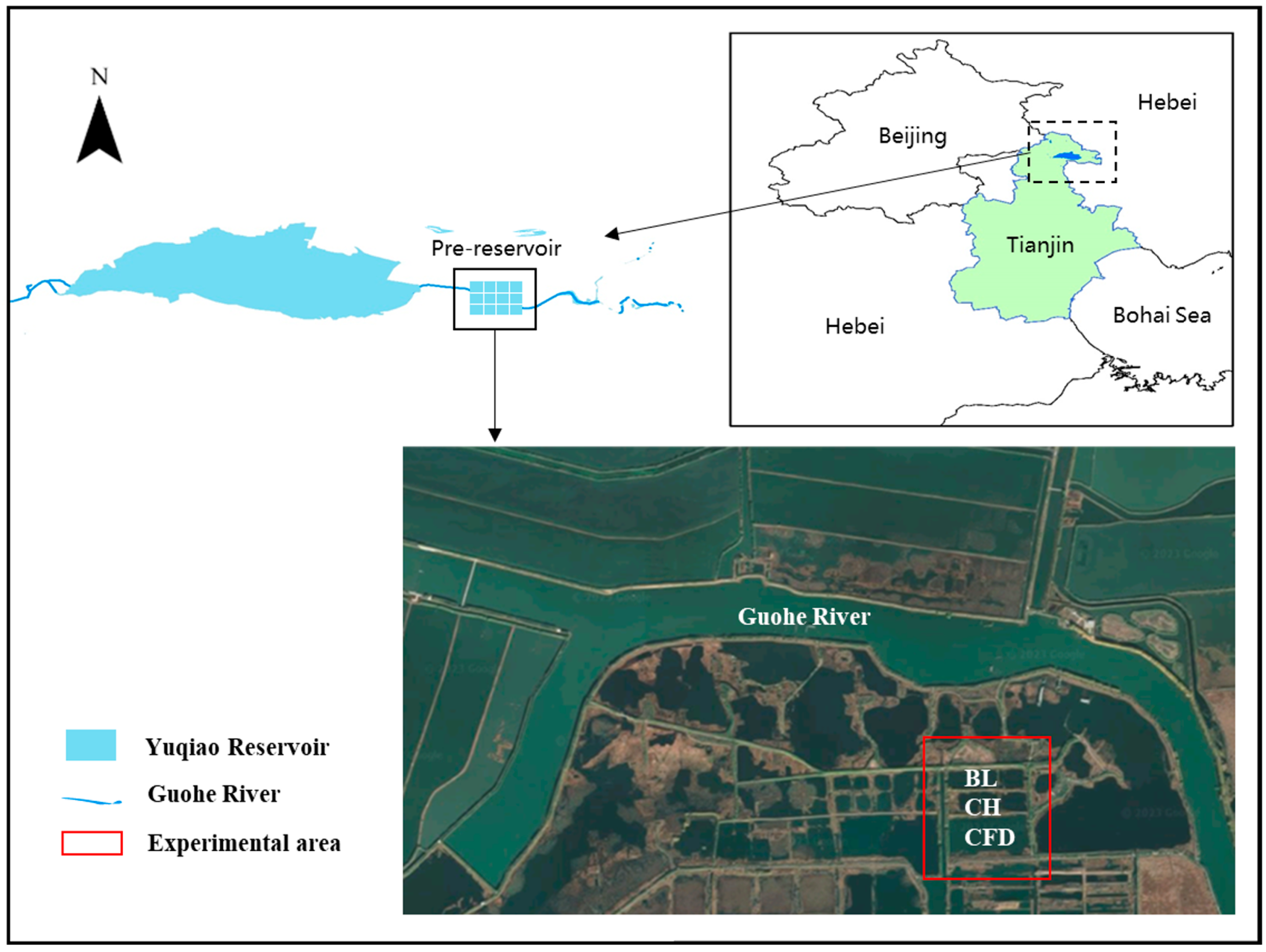
2.1. Study Area

This study was conducted in the Yuqiao Reservoir (117°31′ E, 40°02′ N), located in North China. As a crucial water source for Tianjin, the shallow reservoir significantly contributes to regional biodiversity. With a decline in water quality and ecological health in recent years, the Tianjin authorities established a pre-reservoir system upstream of the river inlet. This system, comprising multiple functional units, aims to intercept pollutants from inflowing rivers, thereby enhancing the reservoir’s ecological environment [13].
The study focused on three ponds within the wetland area of the pre-reservoir (Figure 1), selected to represent different biomanipulation scenarios. These scenarios included: (1) a pond (BL) without any biomanipulation; (2) a pond (CH) where biomanipulation involved the introduction of carnivorous and herbivorous fish; and (3) a pond (CFD) that underwent a more complex biomanipulation strategy involving carnivorous, filter-feeding, and detritus-feeding fish. The ponds, with areas of 4.87 hm2, 4.93 hm2, and 8.60 hm2, were monitored to observe the resulting dynamics in the phytoplankton communities. Baseline surveys of the water’s physicochemical parameters and phytoplankton community structure were initiated in late June 2022 (T1), and subsequent monitoring was carried out periodically.
The study initiated a fish stocking phase in August 2022 in the ponds within the Yuqiao Reservoir area in August 2022. Table 1 details the specific fish species, along with their sizes and densities, that were introduced into each pond. The BL had no fish stocking, distinguishing it from the other ponds. The CH pond included a mix of piscivorous fish including topmouth culter and Chinese perch to control planktivorous fish populations, complemented by herbivorous fish including grass carp and bream for aquatic plant management. The CFD pond employed a diverse array of fish including piscivorous species for predation on planktivorous fish, filter-feeders including silver carp and bighead carp for phytoplankton regulation, and detritivores, specifically Xenocypris carp, to process fish waste and aid in nutrient reduction. Sampling at established sites within each pond was scheduled at subsequent intervals: late September 2022 (T2), late November 2022 (T3), late March 2023 (T4), and early July 2023 (T5).

2.2. Sampling and Analysis

For each sampling session, surface water samples were collected from a depth of 0.5 m at each designated site using a 5 L acrylic water sampler. A liter of each sample was then placed into wide-mouth bottles, preserved with 15 milliliters of Lugol’s iodine solution, and left to settle for 48 h. Subsequently, the sample was concentrated using the siphon method, typically to a tenfold increase. Phytoplankton identification was conducted according to “China Freshwater Algae: System, Ecology, and Classification” [14] and “China Freshwater Biological Atlas” [15]. For counting phytoplankton, the eyepiece field-of-view method was utilized. Once the concentrated sample was mixed, counting was performed in a 0.1 milliliter plankton chamber using an Olympus CX21 optical microscope at 400× magnification. The cell count within the field of view was maintained above 300. Small algae, such as Microcystis spp., which tend to form clusters, were subjected to ultrasonic treatment to disperse the clusters before counting. Each sample was counted in at least two separate chambers, and the average of these counts was recorded as the final count. A count was considered valid if the discrepancy between two chambers did not exceed 15%; if it did, additional counts were made until the result fell within this threshold. The cell counts were then used to calculate phytoplankton densities (cells/L), adjusted for the degree of sample concentration. Measurements of cell morphology, including length, height, and diameter, were taken based on the closest geometric shape for each phytoplankton cell. For each type of cell, at least 50 measurements were conducted. The average of these measurements was used in a formula to calculate cell volume. Given that the density of algae is approximately 1, the biomass (wet weight, mg/L) of the phytoplankton was determined by multiplying the density by the average volume [16].
In conjunction with phytoplankton sampling, additional water quality parameters were assessed. Transparency (SD) was gauged using a Secchi disk, while a suite of parameters including water temperature (WT in °C), dissolved oxygen (DO in mg/L), and pH were measured onsite utilizing a YSI Pro Plus portable multi-parameter water quality analyzer. Concurrently, surface water samples from a depth of 0.5 m were gathered using an acrylic water sampler, immediately homogenized, and subsequently stored in 1 L plastic bottles for further laboratory analysis of key physicochemical parameters. Analytical procedures for total nitrogen (TN in mg/L), total phosphorus (TP in mg/L), and chlorophyll-a (Chl.a in µg/L) were conducted in strict accordance with protocols endorsed by the State Environmental Protection Administration [17].

2.3. Evaluation Indicators

Dominant species were identified using the dominance index (Y) [18], with a species considered dominant if Y > 0.02. The dominance index is calculated by:
Y = Ni × fi/N
where Ni is the number of individuals of the ith phytoplankton species at a sampling site, N is the sum of all phytoplankton individuals at the site, and fi is the frequency of occurrence of that species across all sampling sites.
The Shannon–Wiener diversity index (H′) [19], Simpson’s diversity index (D) [20], Margalef’s richness index (Dm) [21], and Pielou’s evenness index (J′) [22] were used for the quantitative analysis of phytoplankton community diversity. The formulas are as follows:
H   =   i = 1 s P i × l n P i
D = 1   i = 1 s P i 2
D m = ( S 1 ) / l n N
J= H′/lnS
where Pi is the proportion of the ith species, S is the number of species, and N is the total number of individuals of phytoplankton at the sampling sites.
The Trophic Level Index (TLI) method is used to determine the eutrophication status of aquatic environments. This approach uses the chlorophyll-a (Chl.a) concentration as a baseline and integrates a set of water quality parameters—total phosphorus (TP), total nitrogen (TN), and water transparency (SD)—that have minimal absolute deviations. The TLI for each individual parameter is calculated with established equations [23,24]:
T L I C h l . a = 10 2.5 + 1.086 l n C h l . a = 10 2.5 + 0.995 l n C h l . a l n 2.5
T L I T P = 10 9.436 + 1.624 l n T P = 10 9.436 + 1.488 l n T P l n 2.5
  T L I T N = 10 5.453 + 1.694 l n T N = 10 5.453 + 1.552 l n T N l n 2.5
T L I S D = 10 5.118 1.94 l n S D = 10 5.118 1.778 l n S D l n 2.5
The comprehensive TLI, denoted as TLI(Σ), is derived by summing the weighted TLI values of these parameters [23,24]:
T L I Σ = j = 1 m W j × T L I ( j )
W j = r i j 2 / j = 1 m r 2 i j
where TLI(j) is the TLI of the jth parameter; m is the number of parameters; Wj represents the weight factor for the jth parameter’s TLI; and rij is the correlation coefficient between the jth parameter and the benchmark parameter Chl.a.
The trophic status of the ponds is classified according to TLI(Σ) as follows: TLI(Σ) < 30, oligotrophic; 30 ≤ TLI(Σ) ≤ 50, mesotrophic; 50 < TLI(Σ) ≤ 60, light eutrophic; 60 < TLI(Σ) ≤ 70, moderate eutrophic; TLI(Σ) > 70, highly eutrophic. A higher TLI(Σ) within the same trophic status category denotes a more severe degree of eutrophication.

2.4. Statistical Analysis

Physicochemical water quality parameters, phytoplankton density, and biomass were compared across the ponds at different temporal intervals. For datasets conforming to normal distribution and variance homogeneity, one-way repeated-measures ANOVA was applied. The Welch test was reserved for normally distributed data with heteroscedasticity, and the Kruskal–Wallis test was adopted for datasets that did not follow a normal distribution.
Hierarchical clustering of phytoplankton communities in the ponds was performed with the “ComplexHeatmap” package in R version 4.2.2 [25]. The “vegan” package was used for Analysis of Similarities (ANOSIM; n = 999 permutations) to assess significant seasonal differences in community structure. Similarity Percentage Analysis (SIMPER) examined the dissimilarity of phytoplankton communities among the ponds and identified species contributing to differences, with those contributing more than 3% and p < 0.05 considered significant [26].
Detrended Correspondence Analysis (DCA) was conducted on phytoplankton density, with Redundancy Analysis (RDA) selected when the DCA’s longest gradient was less than 3. Key environmental factors were iteratively selected, and their significance on phytoplankton density was evaluated using Monte Carlo tests. Finally, the “rdacca.hp” package in R was used for Hierarchical Partitioning to determine the independent effects and significance of each explanatory variable.

3. Results

3.1. Phytoplankton Species Composition and Dominant Species

A total of 204 phytoplankton species were identified across eight phyla in the ponds: Bacillariophyta, Xanthophyta, Pyrrophyta, Chrysophyta, Cyanophyta, Euglenophyta, Chlorophyta, and Cryptophyta.
In the BL pond, phytoplankton species decreased from 91 at the first sampling (T1) to 73 at the last (T5). The CH pond also saw a reduction from 90 species at T1 to 50 at T5 (Table 2). Conversely, the CFD pond exhibited an increase from 46 species at T1 to 56 at T5. The number of shared species across ponds increased from 25 at T1 to 36 at T5.
The dominant species in each pond, identified using a dominance index (Y ≥ 0.02), varied over time (Table 3). In the BL pond, Microcystis spp. (Cyanophyta) dominated initially (T1–T2), later replaced by Chrysococcus rufescens (Chrysophyta) and Cryptomonas spp. (Cryptophyta) during T3–T4, with a resurgence of Microcystis spp. at T5. The CH pond saw a similar initial dominance by Microcystis spp. and Ceratium spp., with Planktothrix agardhii becoming most prevalent at T3, and Microcystis spp. regaining dominance at T5. The CFD pond had a notable shift from Picocystis dominance at T1 to Cryptomonas spp. from T2 to T4, with Synedra acus emerging as dominant at T5.

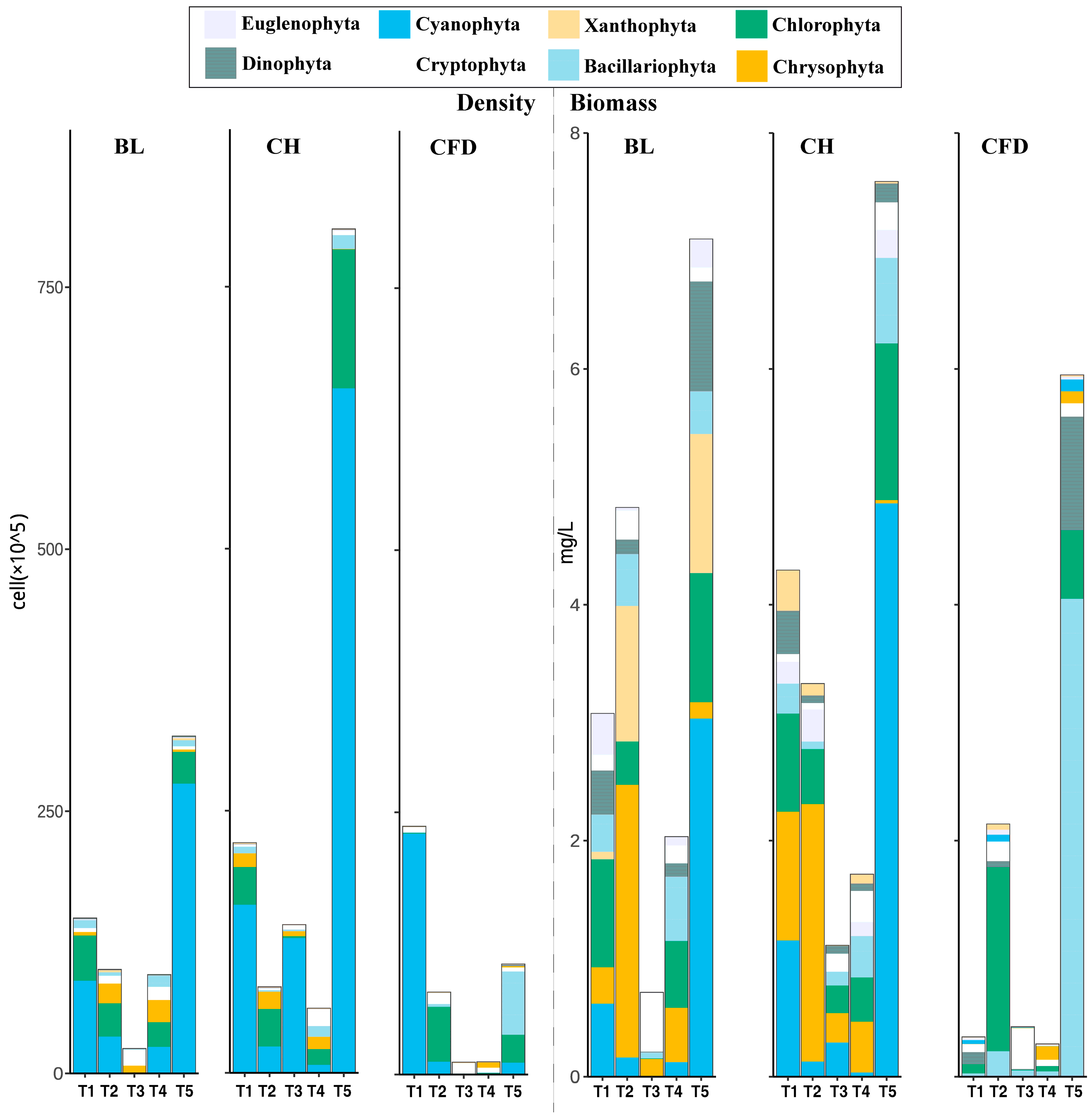
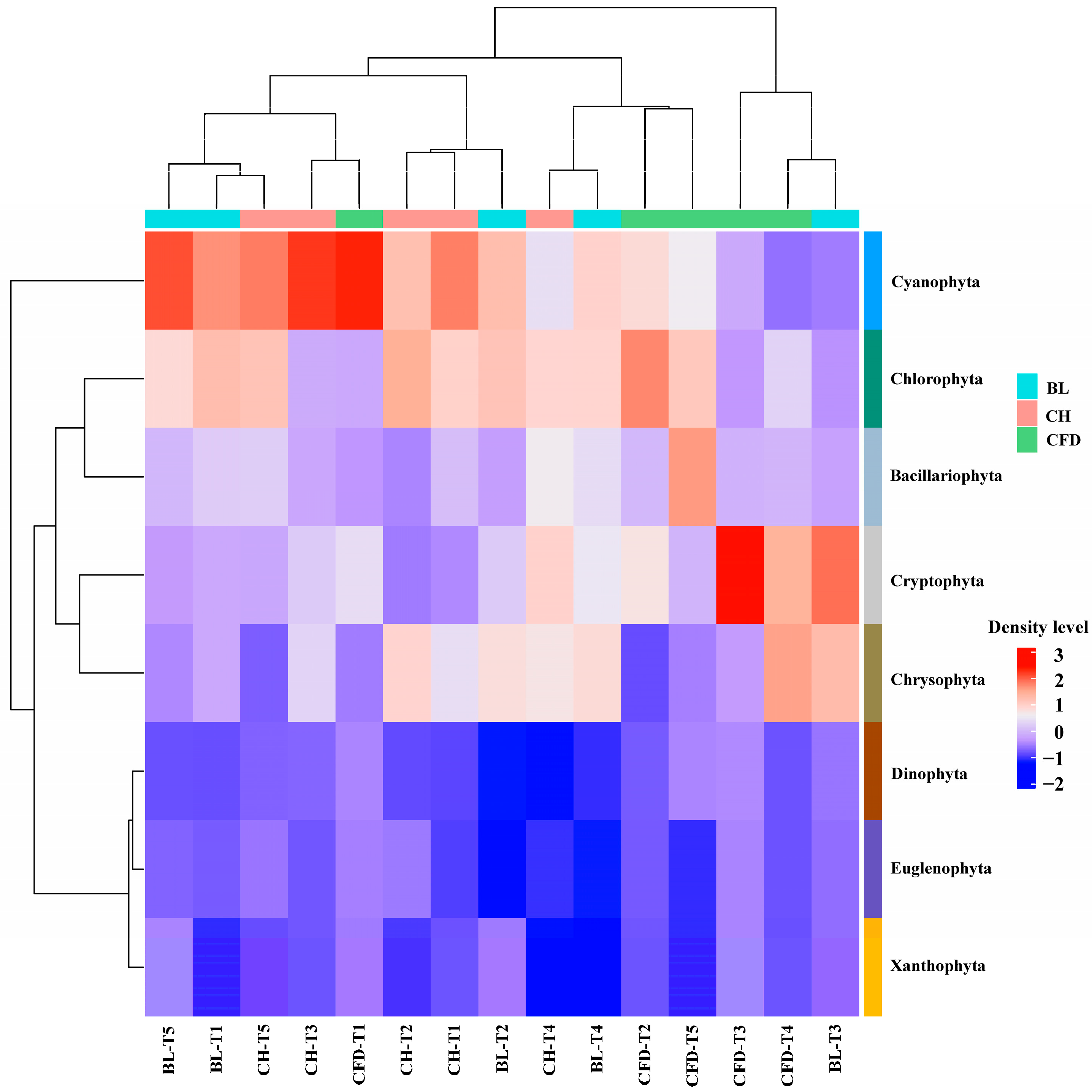
3.2. Phytoplankton Density and Biomass

Phytoplankton density and biomass across the ponds exhibited notable variations throughout the study period (Figure 2). In the BL pond, density ranged from 0.23 × 10⁷ to 3.21 × 10⁷ ind/L, and biomass from 0.71 to 7.10 mg/L. The highest densities were recorded in the summer and autumn periods, dominated by Cyanophyta. The lowest densities occurred in winter, with a predominance of Cryptophyta and Chrysophyta.
In the CH pond, phytoplankton density varied from 0.61 × 10⁷ to 8.04 × 10⁷ ind/L, and biomass from 1.11 to 7.58 mg/L. Cyanophyta were dominant in the T1 period, with a shift to Chlorophyta in T2. The T3 period saw a significant increase in Cyanophyta density, dominating the phytoplankton community. In T4, Cryptophyta, Chlorophyta, and Chrysophyta emerged as major groups, and in T5, Cyanophyta regained dominance.
The CFD pond displayed a range of 0.11 × 10⁷ to 2.36 × 10⁷ ind/L in phytoplankton density and 0.27 to 5.95 mg/L in biomass. The summer of 2022 (T1) marked a period of absolute dominance by Cyanophyta. This was followed by a dominance shift to Chlorophyta in T2 and to Cryptophyta in T3. The T4 period was characterized by a balanced dominance of Chrysophyta and Cryptophyta, while in T5, Bacillariophyta and Chlorophyta emerged as the predominant groups, showcasing a significant alteration in the community structure.
Significant seasonal variations in phytoplankton community density and biomass were observed among the ponds. Analysis of Similarities (ANOSIM) revealed significant differences in phytoplankton community structure between the ponds and across different seasons (p < 0.05). The spatiotemporal clustering analysis, illustrated in Figure 3, categorizes the phytoplankton community structures into three main types: The first type, comprising the BL pond during T3 and the CFD pond during T3 and T4, is characterized by a predominance of Cryptophyta and Chrysophyta. The second type includes the BL and CH ponds in T4, as well as the CFD pond in T2 and T5, distinguished by a high proportion of Chlorophyta, Bacillariophyta, and Cyanophyta. The third type consists of the BL pond in T1, T2, and T5; the CH pond in T1, T2, T3, and T5; and the CFD pond in T1, marked by a high ratio of Cyanophyta and Chlorophyta.
One-way ANOVA analysis of phytoplankton density and biomass across the three ponds revealed distinct seasonal patterns. Initially, at T1, no significant differences were observed in total phytoplankton density, nor in the density and biomass of Cyanophyta and Cryptophyta among the ponds (p > 0.05). Notably, the total biomass in the CFD pond was significantly lower (0.33 mg/L) compared to the BL (3.07 mg/L) and CH (4.29 mg/L) ponds (p < 0.05). This trend was also observed in the biomass of Cyanophyta and both density and biomass of Chlorophyta, where the CFD pond showed significantly lower values than the BL and CH ponds (p < 0.05). No significant differences were found between the BL and CH ponds for these metrics (p > 0.05). By T4, a significant reduction in total phytoplankton density and biomass was recorded in the CFD pond (1.17 × 10⁶ individuals/L and 0.27 mg/L, respectively), markedly lower than in the BL (3.61 × 10⁶ individuals/L and 0.83 mg/L) and CH (6.11 × 10⁶ individuals/L and 1.71 mg/L) ponds (p < 0.05). This trend, excluding Bacillariophyta biomass, persisted across other phytoplankton divisions, with the CFD pond exhibiting significantly lower values than the BL and CH ponds (p < 0.05). In the final sampling period (T5), the CFD pond continued to show significantly lower overall phytoplankton density, Cyanophyta density, and Chlorophyta density compared to the BL and CH ponds (p < 0.05). In contrast, the density and biomass of Bacillariophyta in the CFD pond were significantly higher than in the other ponds (p < 0.05).

3.3. Phytoplankton Community Diversity

Table 4 illustrates the dynamic seasonal changes in phytoplankton community diversity indices. The observed trends from T1 to T4 across the BL, CH, and CFD ponds displayed an initial increase in diversity indices, followed by a contrasting decrease during the T5 period. Notably, while the BL and CH ponds experienced a decline in their diversity indices by T5, the CFD pond showed a marked increase, achieving the highest diversity index among the three ponds by this period. The BL pond exhibited its highest species diversity during T2, as evidenced by the peak in the Shannon–Wiener index, along with the highest values in Simpson’s diversity index and Pielou’s evenness index. This period represented a time of balanced and diverse community structure. However, a significant decrease in these indices during T3 indicated a reduced diversity and evenness in species composition. The CH pond’s diversity indices reached their zenith in T4, with both Simpson’s diversity index and Pielou’s evenness index suggesting enhanced diversity and evenness. This contrasted with the low levels of these indices observed in T3. The CFD pond experienced an increase in the Shannon–Wiener and Simpson’s indices during T2, indicating an enhancement in species diversity and a more evenly distributed community structure. Despite a subsequent decrease in these indices by T5, there was a notable overall improvement in diversity from the initial T1 period, underscoring the effectiveness of the biomanipulation strategy in the CFD pond. This table underlines the fluctuating nature of phytoplankton communities in response to various biomanipulation strategies and changing environmental conditions across seasons.

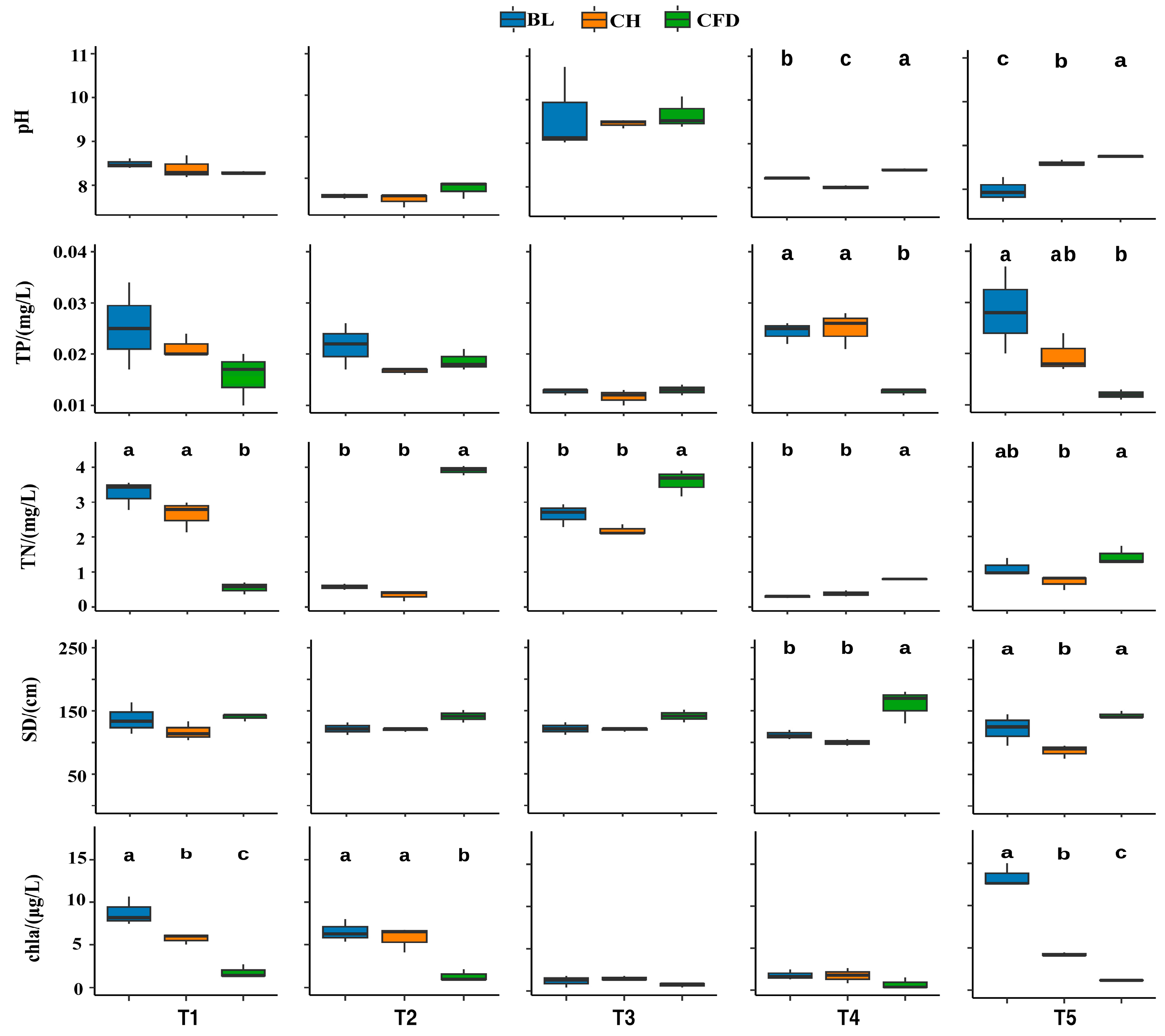
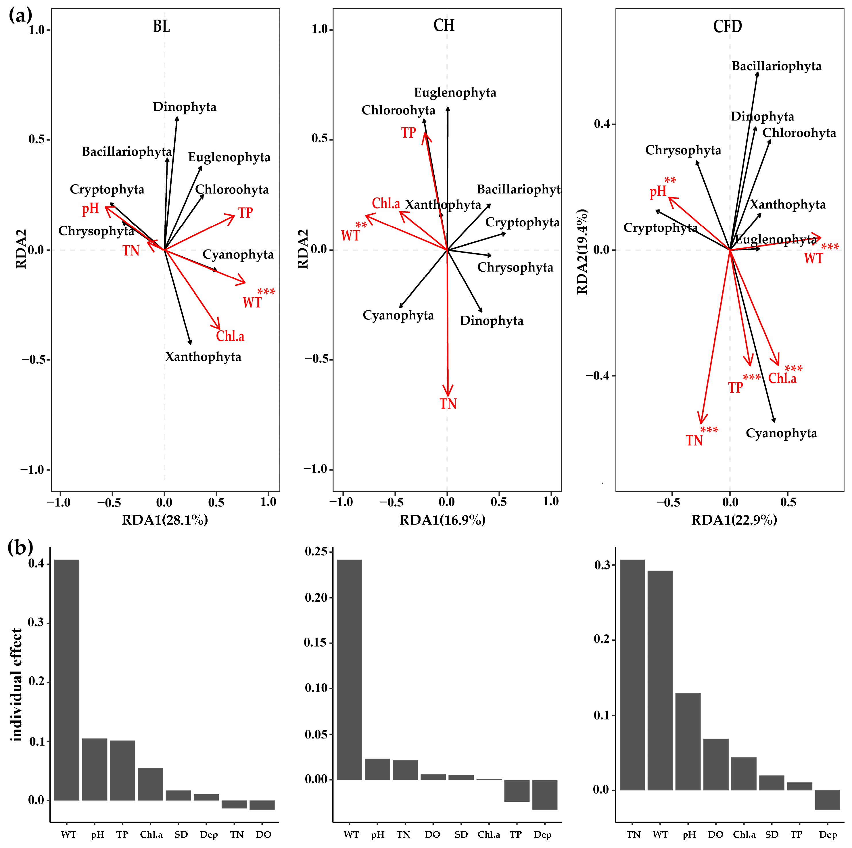
3.4. Relationship between Phytoplankton and Environmental Factors

According to the physicochemical data of the water presented in Figure 4, in the T1 period, there were no significant differences among the three ponds in terms of transparency, pH, total phosphorus, and chlorophyll-a concentration (one-way ANOVA, p > 0.05). However, the total nitrogen content in the CFD pond was significantly lower than that in the BL and CH ponds (p < 0.05). By the T4 period, the CFD pond showed higher values in transparency, pH, and total nitrogen compared to the BL and CH ponds (p < 0.05), while its total phosphorus was significantly lower than these two ponds (p < 0.05). No significant differences were observed in other parameters among the ponds (p > 0.05). In the T5 period, the pH value of the CFD pond was significantly higher than that of the CH pond (p < 0.05), and its concentrations of total phosphorus and chlorophyll-a were significantly lower than those in the BL pond (p < 0.05). These results indicate that there are certain correlations among water environmental factors in experimental ponds under different management measures, which may indirectly affect the structure and distribution of the phytoplankton community.
Figure 5a displays the Redundancy Analysis (RDA) highlighting the correlations between phytoplankton density and environmental factors. In the BL and CH ponds, a significant positive correlation was observed between the density of cyanobacteria and pH levels, contrary to water temperature. For the CFD pond, cyanobacteria density was strongly and positively correlated with total nitrogen, total phosphorus, and chlorophyll-a concentrations (p < 0.01), indicating a substantial influence of these factors on cyanobacterial abundance. Water temperature also exhibited a significant positive association with cyanobacteria density in the CFD pond.
Hierarchical Partitioning analysis, as depicted in Figure 5b, suggests that water temperature was the predominant factor explaining phytoplankton density variation in the BL and CH ponds, accounting for 41.2% and 24.1% of variance, respectively, with both influences reaching statistical significance. Conversely, in the CFD pond, total nitrogen and water temperature were the major contributors to phytoplankton density variation, with significant effects. Other environmental variables, like pH, chlorophyll-a, and total phosphorus, also demonstrated a significant impact on phytoplankton density in the CFD pond, though their contributions were comparatively smaller.

4. Discussion

4.1. Dynamics of Phytoplankton Communities under Different Pond Conditions

The observational study within the Yuqiao Reservoir’s ponds highlights the intricate dynamics of phytoplankton communities under different pond conditions. Our findings align with the existing literature [27,28] showing pronounced seasonal fluctuations in phytoplankton densities, with higher activity in warmer months (summer and autumn) due to favorable temperature conditions that promote algal growth. Conversely, winter’s cooler temperatures correlate with reduced phytoplankton activity, illustrating the temperature’s critical role in influencing algal dynamics.
In the CFD pond, characterized by a mix of carnivorous, filter-feeding, and detritus-feeding fish, a substantial reduction in phytoplankton density and biomass was noted during the T4 period, which could be attributed to the effective biomanipulation strategies employed. This reduction in larger cyanophytes, likely due to the filter-feeding activity and the predation pressure from carnivorous fish, echoes the findings of [29] from the Donghu Lake study. Furthermore, during the T5 period, a significant shift in the phytoplankton community was observed, with a decrease in density but an increase in biomass, suggesting a change in the dominant phytoplankton species.
In the CH pond, stocked with carnivorous and herbivorous fish, an increase in phytoplankton density was particularly evident during the T3 period, with a noticeable proliferation of filamentous algae such as Planktothrix agardhii. This pattern, likely a result of selective zooplankton predation on smaller algal species, aligns with the findings of [30], indicating the relative ineffectiveness of zooplankton grazing on filamentous algae. The increase in harmful algal blooms like Planktothrix agardhii highlights the potential disruptions to the ecological balance of water bodies.
Reflecting on classic biomanipulation strategies [9], the CH pond’s experience during the T5 period, particularly the abundance of Microcystis aeruginosa and Microcystis wesenbergii, suggests an imbalance in fish stocking. The lack of adequate carnivorous fish may have led to insufficient control of algal growth. This observation is supported by [31], emphasizing the need for a significant reduction in planktivorous fish to maintain stable phytoplankton communities. Additionally, the interaction between aquatic plants and phytoplankton, as noted in [32,33], suggests that the introduction of herbivorous fish and the subsequent decrease in aquatic plant coverage could have indirectly promoted phytoplankton growth.
Comparatively, the BL and CH ponds displayed minimal changes in phytoplankton community structure, predominantly dominated by Cyanophyta species. This consistent pattern across seasons, especially in warmer months, can be attributed to the high-temperature tolerance and rapid growth capabilities of Cyanophyta [34]. In stark contrast, the CFD pond exhibited significant shifts in its phytoplankton community, with a marked decrease in Cyanophyta and Chlorophyta and an increase in Bacillariophyta. This trend mirrors the findings from Donghu Lake [29], indicating the effectiveness of the diverse biomanipulation approach in the CFD pond in influencing phytoplankton community dynamics.

4.2. Variations of Phytoplankton Community Diversity and Stability

Significant variations in phytoplankton community diversity were observed throughout the study period, with SIMPER analysis revealing notable dissimilarity among the ponds, ranging from 60.46% to 93.89% (see details in Table A1). These differences underscore the influence of management strategies and seasonal shifts on phytoplankton community structure. In the BL pond, Microcystis spp. and Oscillatoria spp. were the main contributors to community differences. In the CH pond, Ceratium spp. and Microcystis spp. were dominant. For the CFD pond, Picocystis, Dictyosphaerium, Cryptomonas spp., and Microcystis spp. contributed majorly to community differences from T1 to T3, while during T4 to T5, Acutodesmus spp., Pseudanabaena spp., and Chroococcus spp. became the primary contributors. The composition of algal populations and pollution indicator species are important parameters for evaluating the trophic status of lakes. Certain species like Picocystis spp., Microcystis spp., and Planktothrix spp., mainly Cyanophyta, are indicative of eutrophic waters, while species like Scenedesmus spp. and Closterium spp., mostly Chlorophyta, represent mesotrophic to eutrophic waters, and Diatoms and Chrysophytes are more common in oligotrophic waters [35]. During summer, the dominant species in the BL and CH ponds were mainly from Microcystis spp and Scenedesmus spp., typical representatives of eutrophic waters. In contrast, the dominant species in the CFD pond during T4 and T5 were primarily from Chrysophyta and Bacillariophyta, typical of oligotrophic waters.
When the number of dominant species in a community increases and the dominance differences between these species are minimal, the diversity indices are usually higher, indicating greater community stability [36]. The diversity of algal species is also a common indicator for water body classification. Indices like Shannon–Weaver (H′) and Margalef richness (Dm) reflect the complexity of community structures, with higher values indicating greater stability. Pielou’s evenness index (J) reflects the uniformity of species distribution, with higher evenness indicating more uniform distribution. Comparing the phytoplankton diversity indices in summer (T1 and T5 periods) across the ponds [35,37], both the BL and CH ponds showed a decline in diversity indices, particularly a significant drop in Dm, indicating a shift from slightly polluted to β-moderately polluted waters in the BL pond and consistent α-moderate pollution in the CH pond, worsening in the T5 period. In contrast, the CFD pond improved from heavily polluted status in T1 (dominated by Picocystis) to slightly polluted in T5, showing a marked increase in community stability. Overall, the community stability worsened in the BL and CH ponds, while significant improvements in stability and water quality were observed in the CFD pond.

4.3. Assessment of Water Trophic Status and the Potential Role of Biomanipulation

Nitrogen and phosphorus play a critical role in shaping phytoplankton community structures, significantly impacting them. Reducing internal nutrient load, especially phosphorus, is key to successful biomanipulation [38]. At T5, the total phosphorus concentration in the CH pond was slightly lower than in the BL pond, but not significantly different, consistent with observations at T1. This suggests that the CH pond’s influence on total phosphorus concentration was not significant throughout the experiment.
In contrast, the total phosphorus concentration in the CFD pond at T5 was significantly lower than in both the BL and CH ponds. This reduction can be attributed to the filtering action of silver carp and bighead carp, which effectively lower total phosphorus in the water following phytoplankton consumption [39]. Additionally, the stocking of carnivorous fish limited the number of small benthic fish, reducing their disturbance of the sediment and subsequent nutrient resuspension. The stocking of Xenocypris carp might also contribute to nutrient reduction by consuming the excreta of silver carp and bighead carp, further limiting nutrient suspension.
Moreover, the total nitrogen concentration in the BL and CH ponds at T5 significantly decreased compared to T1, while in the CFD pond, it increased. This could be due to the accelerated release of nitrogen in the water following the feeding of silver carp and bighead carp. After these fish feed, most of the nitrogen returns to the water as excreta, entering the nitrogen recirculation process, leading to an increase in total nitrogen concentration [40].
Comparative analysis of the comprehensive Trophic Level Index (TLI) for the three ponds across two successive summers, T1 and T5, is summarized in Table 5. The data reveal that the BL pond exhibited a consistent mild eutrophic status, suggesting a stable nutrient regime and well-regulated phytoplankton dynamics, potentially indicative of a balanced ecosystem. Conversely, the CH pond displayed a transition from mild eutrophic to mesotrophic conditions, hinting at effective nutrient management or adaptive ecological shifts enhancing water quality. The CFD pond, maintaining mesotrophic conditions, showed a minor rise in TLI from 39.9 to 40.8. This nuanced increase points to a potential escalation in total nitrogen levels, which may be attributed to the biotic impacts of introduced fish species on the nitrogen cycle.
These findings highlight the potential benefits of biomanipulation strategies in improving water trophic status. Particularly in the CFD pond, stocking filter-feeding and carnivorous fish significantly reduced total phosphorus concentration and slightly increased the comprehensive nutrient status index, reflecting its potential in alleviating eutrophication. These insights are crucial for water management, suggesting that appropriate biomanipulation strategies can effectively improve water quality and reduce harmful algal blooms. Future research should continue to explore the long-term effects of different biomanipulation strategies on water trophic status to develop more effective water management and restoration strategies.

5. Conclusions

This study offers insights into the dynamics of phytoplankton communities across ponds with varied fish stocking strategies. The results highlight the effectiveness of diversified fish stocking, particularly in the CFD pond, for reducing phytoplankton density and improving water quality, especially in controlling cyanobacteria. The limited impact in ponds with only carnivorous and herbivorous fish suggests that a more integrated approach is essential for effective eutrophication management. The findings emphasize the potential of tailored biomanipulation strategies for aquatic ecosystem restoration, especially in shallow water bodies, and underline the importance of continued research for sustainable ecological balance and water quality improvement.

Author Contributions

Conceptualization, Y.Z., J.Y. and S.Y.; Data curation, Y.Z. and S.Y.; Formal analysis, Y.Z. and S.Y.; Funding acquisition, T.Z. and S.Y.; Investigation, Y.Z., J.Y., X.L., B.T. and S.Y.; Project administration, T.Z. and S.Y.; Resources, J.Y., T.Z. and S.Y.; Supervision, S.Y.; Validation, Y.Z., J.Y., X.L., B.T., T.Z. and S.Y.; Visualization, Y.Z.; Writing—original draft, Y.Z.; Writing—review and editing, Y.Z., J.Y., X.L., B.T., T.Z. and S.Y. All authors have read and agreed to the published version of the manuscript.

Funding

This research was funded by the Tianjin Water Bureau Science and Technology Plan Project, grant number TJRD-2020-B-0142; and the National Natural Science Foundation of China, grant number 32072983, 51679230.

Institutional Review Board Statement

Not applicable.

Data Availability Statement

The data presented in this study are available upon reasonable request from the corresponding author. The data are not publicly available at this moment as the research project to which they belong is currently ongoing. This ensures that the integrity of the ongoing research is maintained and that all data sharing complies with the ethical standards and protocols set forth by our institution.

Acknowledgments

The authors would like to acknowledge the invaluable help of Zhixiang Hao, Jiacheng Wang, Wang Li, and Shiqi Li for their extensive assistance in the study. Additionally, we extend our gratitude to Sen Ding and Xianfu Zhao for their significant contributions and support during the manuscript revision process.

Conflicts of Interest

The authors declare no conflicts of interest. The funders had no role in the design of the study; in the collection, analyses, or interpretation of data; in the writing of the manuscript; or in the decision to publish the results.

Appendix A

Table A1. Seasonal dissimilarity and major contributing species of phytoplankton communities in the ponds within the Yuqiao Reservoir.
PondSeasonal ComparisonDifference%Species 1Contribution%Species 2Contribution%Species 3Contribution%
BL PondT1–T260.46Scenedesmus abundans3.50Scenedesmus quadricauda3.02
T1–T393.89Microcystis aeruginosa9.47Raphidocelis subcapitata5.48Scenedesmus bijuga4.84
T1–T469.44Dactylococcopsis rhaphidioides6.84Chrysococcus diaphanus5.90Kephyrion ovale3.84
T1–T554.57
T2–T383.16Scenedesmus bijuga7.67Raphidocelis subcapitata6.88Dinobryon sertularia6.23
T2–T473.94Dactylococcopsis rhaphidioides7.32Chrysococcus diaphanus5.51Kephyrion ovale3.99
T2–T568.05Microcystis wesenbergii9.58
T3–T469.13Dactylococcopsis rhaphidioides12.32Chroomonas caudata7.46Scenedesmus bijuga6.84
T3–T589.69Microcystis aeruginosa12.43Microcystis wesenbergii10.82Pseudanabaena limnetica6.82
T4–T576.03Microcystis aeruginosa9.21Microcystis wesenbergii8.37Dactylococcopsis rhaphidioides6.45
CH PondT1–T263.41Dinobryon sertularia7.13Dinobryon cylindricum6.45Merismopedia tenuissima4.02
T1–T385.03Microcystis aeruginosa11.36Microcystis wesenbergii6.81Dinobryon cylindricum6.17
T1–T471.69Dinobryon cylindricum5.56Dactylococcopsis rhaphidioides4.51Kephyrion ovale3.99
T1–T554.86Cyclotella ocellata4.86Merismopedia tenuissima3.79Scenedesmus aculeolatus3.78
T2–T385.92Dinobryon sertularia9.24Scenedesmus bijuga9.11Pseudanabaena limnetica7.71
T2–T481.33Dinobryon sertularia6.80Chroomonas acuta5.55Achnanthes exigua5.01
T2–T572.15Microcystis aeruginosa10.46Microcystis wesenbergii9.61Oscillatoria amphibia9.35
T3–T472.26Dactylococcopsis rhaphidioides7.72Achnanthes exigua7.59Chroomonas acuta6.72
T3–T588.98Microcystis aeruginosa12.64Oscillatoria amphibia10.47Microcystis wesenbergii9.78
T4–T577.71Microcystis aeruginosa11.09Oscillatoria amphibia9.32Microcystis wesenbergii8.71
CFD PondT1–T278.84Scenedesmus bijuga9.88Raphidocelis subcapitata5.77Coelastrum reticulatum4.75
T1–T374.54Merismopedia minima47.77Chroomonas caudata16.55Microcystis aeruginosa7.66
T1–T477.34Merismopedia minima41.59Kephyrion ovale11.69Microcystis aeruginosa7.40
T1–T583.55Synedra acus11.92Cyclotella ocellata8.22Chlorella vulgaris6.14
T2–T381.82Scenedesmus bijuga11.00Raphidocelis subcapitata6.40Coelastrum reticulatum5.73
T2–T485.96Scenedesmus bijuga9.91Microcystis aeruginosa5.29Raphidocelis subcapitata5.21
T2–T565.87
T3–T463.62Chroomonas caudata24.06Kephyrion ovale20.08Chrysococcus diaphanus8.04
T3–T585.96Synedra acus13.71Cyclotella ocellata9.27Chlorella vulgaris7.30
T4–T586.30Synedra acus12.96Cyclotella ocellata8.30Chlorella vulgaris6.63

References

  1. Schindler, D.W. Recent advances in the understanding and management of eutrophication. Limnol. Oceanogr. 2006, 51, 356–363. [Google Scholar] [CrossRef]
  2. Conley, D.J.; Paerl, H.W.; Howarth, R.W.; Boesch, D.F.; Seitzinger, S.P.; Havens, K.E.; Lancelot, C.; Likens, G.E. Controlling eutrophication: Nitrogen and phosphorus. Science 2009, 323, 1014–1015. [Google Scholar] [CrossRef]
  3. Søndergaard, M.; Jensen, J.P.; Jeppesen, E. Role of sediment and internal loading of phosphorus in shallow lakes. Hydrobiologia 2007, 581, 373–385. [Google Scholar] [CrossRef]
  4. Smith, V.H.; Schindler, D.W. Eutrophication science: Where do we go from here? Trends Ecol. Evol. 2009, 24, 201–207. [Google Scholar] [CrossRef]
  5. Carpenter, S.R.; Kitchell, J.F.; Hodgson, J.R. Cascading trophic interactions and lake productivity. BioScience 1985, 35, 634–639. [Google Scholar] [CrossRef]
  6. McQueen, D.J. Manipulating lake community structure: Where do we go from here? Freshw. Biol. 1990, 23, 613–620. [Google Scholar] [CrossRef]
  7. Jeppesen, E.; Søndergaard, M.; Søndergaard, M.; Christoffersen, K. (Eds.) The Structuring Role of Submerged Macrophytes in Lakes; Springer: New York, NY, USA, 1997. [Google Scholar]
  8. Liu, J.K.; Xie, P. Unraveling the enigma of the disappearance of water bloom from the East Lake (Lake Donghu) of Wuhan. Resour. Environ. Yangtze Basin 1999, 3, 85–92. [Google Scholar]
  9. Dionisio Pires, L.M.; Ibelings, B.W.; Brehm, M.; Van Donk, E. Comparing Grazing on Lake Seston by Dreissena and Daphnia: Lessons for Biomanipulation. Microb. Ecol. 2005, 50, 242–252. [Google Scholar] [CrossRef]
  10. Søndergaard, M.; Jeppesen, E.; Lauridsen, T.L. Lake restoration: Successes, failures and long-term effects. J. Appl. Ecol. 2008, 45, 782–797. [Google Scholar] [CrossRef]
  11. Qin, B.Q.; Xu, P.Z.; Wu, Q.L.; Luo, L.C.; Zhang, Y.L. Environmental issues of lake Taihu, China. Hydrobiologia 2007, 581, 3–14. [Google Scholar] [CrossRef]
  12. Zhang, Y.; Qin, B.; Chen, W.; Zhu, G. A study of the diatom assemblages in the sediments of the northern part of Taihu Lake, China. J. Paleolimnol. 2010, 43, 415–426. [Google Scholar]
  13. Fu, Z.Y. Application of pre-reservoir in water resource allocation and water environment protection of Yuqiao Reservoi. Haihe Water Resour. 2019, 1, 44–45. [Google Scholar]
  14. Hu, H.J.; Wei, Y.X. The Freshwater Algae of China-Systematics, Taxonomy and Ecology, 1st ed.; Science Press: Beijing, China, 2006; pp. 1–1023. [Google Scholar]
  15. Han, M.S.; Shu, Y.F. Chinese Freshwater Organisms Atlas, 1st ed.; Ocean Press: Beijing, China, 1995; pp. 1–390. [Google Scholar]
  16. Huang, X.F. Survey, Observation and Analysis of Lake Ecology, 1st ed.; Standards Press of China: Beijing, China, 2000; pp. 72–77. [Google Scholar]
  17. The State Environmental Protection Administration. Water and Wastewater Monitoring and Analysis Method, 4th ed.; China Environmental Science Press: Beijing, China, 2002; pp. 1–836. [Google Scholar]
  18. Dufrêne, M.; Legendre, P. Species Assemblages and Indicator Species: The Need for a Flexible Asymmetrical Approach. Ecol. Monogr. 1997, 67, 345–366. [Google Scholar] [CrossRef]
  19. Shannon, C.E. A mathematical theory of communication. Bell Syst. Tech. J. 1948, 27, 379–423. [Google Scholar] [CrossRef]
  20. Simpson, E.H. Measurement of Diversity. Nature 1949, 163, 688. [Google Scholar] [CrossRef]
  21. Margalef, R. Information theory in ecology. Gen. Syst. 1958, 3, 36–71. [Google Scholar]
  22. Pielou, E.C. Species-diversity and pattern-diversity in the study of ecological succession. J. Theor. Biol. 1996, 10, 370–383. [Google Scholar] [CrossRef] [PubMed]
  23. Jin, X.C.; Tu, Q.Y. Specification For Lake Eutrophication Survey, 2nd ed.; China Environmental Science Press: Beijing, China, 1990; pp. 286–291. [Google Scholar]
  24. Wang, M.C.; Liu, X.Q.; Zhang, J.H. Evaluate method and classification standard on lake eutrophication. Environ. Monit. China 2002, 18, 47–49. [Google Scholar]
  25. R Core Team. R: A Language and Environment for Statistical Computing, Reference Index Version 4.2.2; R Foundation for Statistical Computing: Vienna, Austria, 2022; Available online: https://www.R-project.org/ (accessed on 20 November 2023).
  26. Clarke, K.R. Non-parametric multivariate analyses of changes in community structure. Aust. J. Ecol. 1993, 18, 117–143. [Google Scholar] [CrossRef]
  27. Nie, Y. Phytoplankton Community Structure and Eutrophication Status in Yuqiao Reservoir. Master’s Dissertation, Tianjin University of Science and Technology, Tianjin, China, 2016. [Google Scholar]
  28. Gao, K.; Li, Z.L.; Zhao, X.H.; Zhang, X.X.; Mei, P.W.; Zhang, Z. Spatiotemporal dynamics of and influencing factors on the phytoplankton community in the Yuqiao Reservoir. J. Agric. Resour. Environ. 2023, 1–19. Available online: https://link.cnki.net/urlid/12.1437.s.20230811.1642.002 (accessed on 20 November 2023).
  29. Liu, J.K.; Xie, P. Direct control of microcystis bloom through the use of Planktivorous Carp-closure Experiments and Lake Fishery. Ecol. Sci. 2003, 3, 193–198. [Google Scholar]
  30. Ghadouani, A.; Pinel-Alloul, B.; Prepas, E.E. Effects of experimentally induced cyanobacterial blooms on crustacean zooplankton communities: Cyanobacteria effects on herbivores. Freshw. Biol. 2003, 48, 363–381. [Google Scholar] [CrossRef]
  31. Mehner, T.; Kasprzak, P.; Wysujack, K.; Laude, U.; Koschel, R. Restoration of a stratified lake (Feldberger Haussee, Germany) by a combination of nutrient load reduction and long-term biomanipulation. Int. Rev. Hydrobiol. 2001, 86, 253–265. [Google Scholar] [CrossRef]
  32. Wu, Z.B.; Qiu, D.R.; He, F.; Fu, G.P.; Cheng, S.P.; Ma, J.M. Effects of rehabilitation of submerged macrophytes on nutrient level of a eutrophic lake. Chin. J. Appl. Ecol. 2003, 14, 1351–1353. [Google Scholar]
  33. Shi, X.L.; Yang, J.S.; Chen, K.N.; Zhang, M.; Yang, Z.; Yu, Y. Review on the control and mitigation strategies of lake cyanobacterial blooms. J. Lake Sci. 2022, 34, 349–375. [Google Scholar]
  34. Ma, J.R.; Deng, J.M.; Qin, B.Q.; Long, S.X. Progress and prospects on cyanobacteria bloom-forming mechanism in lakes. Acta Ecol. Sin. 2013, 33, 3020–3030. [Google Scholar]
  35. Kuang, Q.J.; Ma, P.M.; Hu, Z.Y.; Zhou, G.J. Study on the evaluation and treatment of lake eutrophication by means of algae biology. J. Saf. Environ. 2005, 2, 87–91. [Google Scholar]
  36. Jia, H.Y.; Xu, J.F.; Lei, J.S. Relationship of community structure of phytoplankton and environmental factors in Danjiangkou Reservoir bay. Yangtze River 2019, 50, 52–58. [Google Scholar]
  37. Bai, L.J.; Zhang, Z.Y.; Wang, L.; Zhou, B.B.; Li, Y.C.; Shao, X.D.; Su, S.; Liu, Q. Analysis of plankton community and fishery resources in Xiangshui Reservoir. J. Dalian Ocean. Univ. 2020, 35, 280–287. [Google Scholar]
  38. Drenner, R.W.; Hambright, R.K.D. Piscivores, Trophic Cascades, and Lake Management. Sci. World J. 2002, 2, 284–307. [Google Scholar] [CrossRef]
  39. Cui, F.Y.; Lin, T.; Ma, F.; Zhang, L.Q. Experimental Studies on Biomanipulation of Silver Carp and Bighead Carp in Water Resources Management. J. Nanjing Univ. Sci. Technol. 2004, 06, 668–672. [Google Scholar]
  40. Chen, S.L.; Liu, X.F.; Hua, L. The role of Silver carp and Bighead in the cycling of Nitrogen and Phosphorus in the East Lake ecosystem. Acta Hydrobiol. Sin. 1991, 1, 8–26. [Google Scholar]
Figure 1. Location and configuration of the ponds within the Yuqiao Reservoir Wetland Region in Tianjin, China. The ponds, highlighted within the pre-reservoir system, are marked as BL (pond with no fish stocking, serving as a reference point), CH (pond stocked with carnivorous and herbivorous fish), and CFD (pond stocked with a suite of fish including carnivorous, filter-feeding, and detritus-feeding species).
Diversity 16 00075 g001
Figure 2. Seasonal changes in phytoplankton community density and biomass in the ponds.
Diversity 16 00075 g002
Figure 3. Heatmap of phytoplankton density and spatiotemporal clustering across the ponds.
Diversity 16 00075 g003
Figure 4. Variation of key water quality parameters in the ponds over time, with letter annotations (a, b, c) indicating levels of statistical significance; different letters denote significant differences and identical letters indicate no significant difference.
Diversity 16 00075 g004
Figure 5. (a) Redundancy Analysis (RDA) illustrating the influence of environmental factors (red lines) on phytoplankton density, and (b) Hierarchical Partitioning Analysis assessing the independent effects of these factors in the ponds. TN: total nitrogen; TP: total phosphorus; WT: water-temperature; Chl.a: chlorophyll-a; SD: transparency; Dep: water depth; DO: dissolved oxygen. “**” indicates p < 0.01; “***” indicates p < 0.001.
Diversity 16 00075 g005
Table 1. Sizes and densities of fish species stocked in the ponds within the Yuqiao Reservoir.
Fish SpeciesSize of Stocked Fish (cm)Density of Stocked Fish (ind/hm2)
CH Pond 1CFD Pond 2
Topmouth culter (Culter alburnus)5120120
Chinese perch (Siniperca chuatsi)106060
Grass carp (Ctenopharyngodon idellus)8105
Bream (Megalobrama amblycephala)5300
Silver carp (Hypophthalmichthys molitrix)20 225
Bighead carp (Aristichthys nobilis)20 75
Yellow tail (Xenocypris microlepis)9 225
1 Stocked with carnivorous and herbivorous fish. 2 Stocked with carnivorous, filter-feeding, and detritus-feeding fish.
Table 2. Number of phytoplankton species and shared species in the ponds over the five sampling periods.
Time PeriodNumber of Species in BL Pond 1Number of Species in CH Pond 2Number of Species in CFD Pond 3Number of Shared Species
T1 (Late June 2022)91904625
T2 (Late September 2022)71657329
T3 (Late November 2022)37383617
T4 (Late March 2023)72734129
T5 (Early July 2023)73505636
Total16215913199
1 Without fish stocking. 2 Stocked with carnivorous and herbivorous fish. 3 Stocked with carnivorous, filter-feeding, and detritus-feeding fish.
Table 3. Dominant phytoplankton species composition and dominance indices in the ponds over the five sampling periods.
Dominant SpeciesBL Pond 1CH Pond 2CFD Pond 3
T1T2T3T4T5T1T2T3T4T5T1T2T3T4T5
Cyanophyta
Microcystis aeruginosa0.430.14 0.310.590.04 0.55 0.05
Pseudanabaena limnetica 0.03 0.040.020.040.89 0.02
Cylindrospermum majus 0.03 0.14
Microcystis wesenbergii0.06 0.07 0.11
Microcystis marginata 0.03
Merismopedia minima0.040.03 0.04 0.96 0.52
Merismopedia tenuissima0.04 0.04
Dactylococcopsis rhaphidioides 0.250.03 0.11
Oscillatoria amphibia
Dolichospermum bergii 0.02
Bacillariophyta
Achnanthes exigua0.03 0.05 0.11
Synedra acus 0.02 0.03 0.03 0.45
Cyclotella ocellata 0.12
Chrysophyta
Dinobryon cylindricum 0.05
Dinobryon sertularia 0.16 0.02 0.20
Kephyrion ovale 0.03 0.05 0.08 0.29
Chrysococcus diaphanus 0.27 0.16 0.03 0.05 0.09
Dinobryon divergens 0.03 0.04
Dinobryon bavaricum 0.03
Chlorophyta
Raphidocelis subcapitata0.07 0.09 0.04 0.040.04 0.10 0.03 0.02 0.07
Scenedesmus abundans0.03
Scenedesmus bijuga0.05 0.12 0.07 0.04 0.23 0.06 0.06 0.25 0.05
Crucigenia quadrata0.03 0.03 0.08 0.06 0.04
Scenedesmus quadricauda0.02 0.02 0.03
Crucigenia tetrapedia 0.03 0.02 0.03 0.04
Coelastrum reticulatum 0.05
Coelastrum microporum 0.04
Planctonema lauterbornii 0.04
Chlorella vulgaris 0.06 0.07
Schroederia setigera 0.05
Cryptophyta
Chroomonas acuta 0.02 0.31 0.13 0.04 0.22 0.11 0.42 0.35 0.03
Chroomonas caudata 0.03 0.33 0.02 0.46
1 Without fish stocking. 2 Stocked with carnivorous and herbivorous fish. 3 Stocked with carnivorous, filter-feeding, and detritus-feeding fish.
Table 4. Temporal dynamics of phytoplankton community diversity indices in the ponds.
PondTime
Period
Shannon–Wiener
Diversity Index (H′)
Simpson’s
Diversity Index (D)
Margalef’s
Richness Index (Dm)
Pielou’s
Evenness Index (J)
BL PondT12.540.7976.340.56
T22.990.9205.070.70
T31.540.7242.910.43
T42.700.8805.160.63
T51.710.6884.810.40
CH PondT11.900.6376.100.42
T22.520.8684.700.60
T30.630.2022.610.17
T42.920.9085.400.68
T51.530.6523.650.37
CFD PondT10.230.0753.070.06
T22.890.9035.310.67
T31.320.6103.010.37
T42.090.7803.430.56
T52.270.7703.970.56
T1: late June 2022; T2: late September 2022; T3: late November 2022; T4: late March 2023; T5: early July 2023.
Table 5. Comparison analysis of the comprehensive Trophic Level Index (TLI) across consecutive summers in the ponds.
Time PeriodBL PondCH PondCFD Pond
T1 (Late June 2022)50.452.139.9
T5 (Early July 2023)52.346.440.8
Disclaimer/Publisher’s Note: The statements, opinions and data contained in all publications are solely those of the individual author(s) and contributor(s) and not of MDPI and/or the editor(s). MDPI and/or the editor(s) disclaim responsibility for any injury to people or property resulting from any ideas, methods, instructions or products referred to in the content.

