
The Relationship between Inbreeding and Fitness Is Different between Two Genetic Lines of European Bison

Department of Animals Genetics and Conservation, Warsaw University of Life Sciences, Ciszewskiego 8, 02-786 Warsaw, Poland
Diversity 2023, 15(3), 368; https://doi.org/10.3390/d15030368
Submission received: 21 December 2022
/
Revised: 27 February 2023
/
Accepted: 3 March 2023
/
Published: 4 March 2023
(This article belongs to the Special Issue Conservation of Bison Populations – Achievements and Problems)
Abstract
:The pedigree data for European bison are published in the European Bison Pedigree Book, established one hundred years ago. The species passed a serious bottleneck and was kept in captivity for more than 30 years. After reintroduction, some individuals were captured and moved to enclosures, which caused gaps in pedigree data. To prevent the underestimation of inbreeding value, only animals with a fully known pedigree were used in the analysis. European bison were divided into two genetic lines, Lowland-Caucasian (LC) and Lowland (LB), with different numbers of founders (all 12 vs. 7 of them). The relation between inbreeding and survival up to one month of age, calculated using logistic regression, gave different results for every genetic line. In the LC line (N = 5441), the average inbreeding level was equal to 0.253 and the influence into survival was negative (exp(B) = 0.190), but in the LB line (N = 1227), the inbreeding level was much higher (0.410) but the influence into survival was positive (exp(B) = 6.596). It could be assumed that the difference between lines is a result of purging in the first period of species restitution.
Keywords:
inbreeding depression; survival; genetic line; European bison; pedigree analysis; founders1. Introduction
Wisent or European bison (Bison bonasus) is a species that passed a serious bottleneck and, in consequence, matings between relatives are inevitable. At the same time, the fertility and survival rate of the species, both determining its population growth, are supposedly not affected. Almost 100 years ago, this species was drastically reduced and all natural populations disappeared—in the Białowieska Forest in 1919 [1], and in the Caucasus Mountains in 1927 [2]. At the end of 1924, only 54 animals (29 males and 25 females) lived in European zoos and enclosures [2,3]. The world population of European bison initially increased very slowly, but later the increase rate of the population was much larger. Presently, the wisent population has reached over 9500 individuals, including nearly 2300 kept in captivity [4]. Due to the very limited genetic variability, the European bison are a unique subject for studying inbreeding issues.
All living wisents are descendants of 12 founders [5,6,7]. Eleven of them belong to the lowland subspecies Bison bonasus bonasus and only one male to the subspecies Bison bonasus caucasicus. Every animal with this particular founder in the pedigree belongs to the Lowland-Caucasian (LC) line. Wisents with lowland founders only are included in the lowland line (LB). The LC line is derived from all 12 founders. This line could be called open, because only one parent belonging to this line is sufficient for the descendant to also belong to it [8]. The lowland line (LB) comes from the seven founders [7], of which the founding pair 42 PLANTA and 45 PLEBEJER have the largest contribution. Within the lowland line, there can be distinguished the so-called “Pszczyna” subline, derived from those two founders only [9,10]. The proportion of both lines in captive herds is not equal; in contemporary populations, the percentage of animals belonging to the LC line is almost two times larger than the LB line [4]
The consequence of the small number of founders and their uneven representation is a high relationship and inbreeding level. The values of the inbreeding coefficient, calculated many years ago [5,11], were between 0.160 to 0.331 and were much lower than those calculated later. In more contemporary research, the values of the inbreeding coefficient were larger [12,13,14], up to 0.57 for the LB line [15]. The values of the inbreeding coefficient are constantly growing but the inbreeding depression is barely visible. Some authors explained that inbreeding could not be deleterious for the growth of the population of endangered species as the European bison is [16,17].
Some connections between inbreeding and various traits were studied in this species. In some studies, the negative effect of inbreeding on the viability of young animals has been found [5,11,12,18]. The lines also have different levels of inbreeding influence [19]. A directly proportional relationship was also found between the level of a female inbreeding and the length of the interval between calving [11] and the sex ratio [20]. A negative effect of inbreeding on the growth parameters of the European bison skeleton was found, more strongly expressed in the LC line and in females. As the inbreeding value increases, the skullcap becomes shorter and the skull base lengthens [21]. Another negative effect was the relationship between the level of inbreeding and the existence of cysts in the male genital organs [14]. It has been suggested that the decreased resistance of European bison to diseases is related to inbreeding [22], but this finding has not been supported by research results.
Many papers present, in captive populations, the problem of the inbreeding level and its consequences as inbreeding depression on viability [23,24]. Inbreeding depression could be explained as a decrease in the level of traits among individuals derived from relatives’ mating. Charles Darwin noticed that plants obtained by self-pollination grew slower, had less weight, bloomed later and produced fewer seeds [25]. Inbreeding depression is expressed very differently but the negative effects of inbreeding on reproduction and viability are well known. Depression was initially studied in populations of laboratory and domestic animal species [25,26]. Inbreeding has been confirmed to be the cause of the extinction of the Melitaea cinxia butterfly population [27,28]. Research about the costs of inbreeding for wild animal species was performed very often in captivity [23,24,29] and also for natural populations, where the level of homozygosity was possible to evaluate [30]. However, the inbreeding level is difficult to evaluate in wild populations, where pedigrees are unknown [31]. In recent years, DNA tests have made it possible to assess the degree of homozygosity of individuals and compare the survival and reproduction parameters of animals with different degrees of homozygosity [32]. The harmful effects of inbreeding on fitness are well known for many species, and papers based on the evaluation of homozygosity show even greater impacts on individual fitness than those based on pedigree analysis [33].
Studies about inbreeding also take into account various types of possibilities to avoid the problem of depression. One of these is purging, which means more effective natural selection against the deleterious alleles due to inbreeding, which can be beneficial for some populations [34,35,36,37]. Although the purging of lethal or semi-lethal alleles may occur, it does not mean that all causes of inbreeding depression will disappear. Theoretically, more homozygotes offer the possibility to eliminate recessive genes very efficiently, but because of small sample sizes, short study durations, etc., there are not many studies providing evidence of the significance of purging in wild populations [38,39,40]. The lower influence of inbreeding upon general fitness is also explained by the purging of deleterious alleles from a population [36,41,42].
The primary and most reliable sources of information about the genetic variability of the European bison are their pedigrees, which have been published in the European Bison Pedigree Book (EBPB) for longer than 100 years. The Pedigree Book’s goal was to register only pure European bison born in captive herds. The reason was the danger of crossbreeding with American bison (Bison bison), kept in many places in Europe [13]. When reintroduced populations became larger, some animals were captured and used for breeding in captivity [43]. They were registered in the Pedigree Book without known parents, but, because all reintroduced populations originated from captivity, such animals could not be counted as founders. For some analyses, the pedigree data of animals captured from free herd in the Białowieska Forest were assumed [19] but this did not change the conclusion.
Thanks to information about dates of birth and death included in the EBPB, it was possible to find data on animals’ survival to the age of one month. According to the survival curve [19], the mortality rate in the first month of age is a few times larger than in the next months, and these values do not depend on a breeder. The mortality in European bison calves is very low compared to other species. The mortality rate estimated in free-roaming herds in the Białowieska Forest (2.8 to 3.2%) is much lower than in enclosures, mainly because, in nature, it is not possible to note stillbirths and very early deaths. In enclosures, the level of mortality in the first 30 days exceeds 10% [44,45]. European bison are seasonal animals so most calves are born from May to July [19,46], and the sex ratio does not differ significantly from the proportion 1:1 [45].
The aim of this paper was to present the level of inbreeding within both genetic lines and to analyze inbreeding’s impact on survival in the first month of life, as a trait representing the fitness of the species.
2. Materials and Methods
The material for the analysis was information about European bison individually registered in the European Bison Pedigree Book (EBPB), from the first issue [3] to the end of the year 2021 inclusive [4,47]. Information included in the Pedigree Book includes an individual’s number, the sex of the individual, data about parents, and the dates of its birth and death. For every individual, the information about its genetic line (LB or LC) was verified with the pedigree.
In total, 13,570 European bison were born before 2022 and individually registered in the EBPB.
On the basis of the pedigree, the inbreeding coefficient of each individual was calculated using our own software, developed for previous studies [19,48] based on the tabular method developed by Henderson and Quass [49]. This method of inbreeding calculation included all generations between the founders and individual. In parallel, the contribution of twelve founders was also calculated for every individual. The sum of these contributions was the level of known pedigree of the individual. For this analysis, only animals with a fully known pedigree (the sum of all founders’ contributions was equal to 100%) and born in the years 1946–2021 were considered (N = 6868), so as to avoid underestimation of the inbreeding coefficient and the lack of information in the years before 1946. The reason for gaps in pedigree—and, in consequence, the lower sum of all founders’ contribution—was the use of captive breeding animals captured from free-roaming herds. Almost half of the captured animals left offspring individually registered, but consequently with partly or completely unknown pedigrees. The inbreeding coefficient calculated for animals with gaps in pedigree was underestimated and not comparable. For every animal, information about its survival up to the first month of life was added as a binomial trait. The age of one month was chosen based on the survival curve [19]. Because survival depends on the season of birth, animals were divided into three groups: the first born in the Spring season (months from April to July), the second born in the Autumn season (from August to November) and the third born in the Winter season (from December to March). Another considered feature was the sex of the animal. Differences between genetic lines in male frequency were checked using the Chi-square test.
The average values of inbreeding coefficients for every year of birth, as well as the inbreeding distribution within every genetic line, are presented in the graphs.
The frequency of survival of European bison was analyzed using generalized binary models, with the dependent variable being survival up to the age of one month (marked as 1 for survived and marked as 0 for dead at this age). The explanatory variables in all models were the sex, season of birth and inbreeding coefficient of an individual. The Wald χ2 was used to determine whether explanatory variables in a model were significant. As the result of the binary models, we presented both B and EXP(B) values. The B value equal to zero (EXP(B) = 1) indicates no difference between the compared levels of the explanatory variable. The EXP(B) presents the probability of survival in comparison to the basic level of the explanatory variable. The basic levels were males in terms of sex, Winter in terms of the season of birth and a value of zero for inbreeding.
Three logistic regressions were performed: (A) for all individuals, (B) for individuals belonging to the Lowland line (LB), (C) for individuals belonging to the Lowland-Caucasian line (LC). Analyzed were only animals born between years 1946 and 2021 and with a full known pedigree. Records that were doubtful or with missing data (sex or no information about birth season) were excluded from the analysis. All statistical analyses were performed using the IBM SPSS statistics software (version 28.0.1.0).
3. Results
The number of animals and their distribution in genetic lines, with average values of survival and the percentage of males, are presented in Table 1.
The total number of analyzed animals (with known pedigree in 100%) was 6868, divided into two lines: LC with 5641 and LB with 1227 animals. The survival rate until the first month of age was equal to 88.1% (Table 1), slightly larger in the LB line (90.3%) than in the LC line (87.6%), and the difference between lines was significant (Χ2 = 6.88; p = 0.009). The sex proportion was also not the same within lines but the difference was not significant (Χ2 = 3.04; p = 0.081).
The averages of the inbreeding coefficient within the analyzed group of animals are given in Table 2. The number of generations from founders to individuals was between 3 and 14, on average 7.48 (s.d. = 1.97).
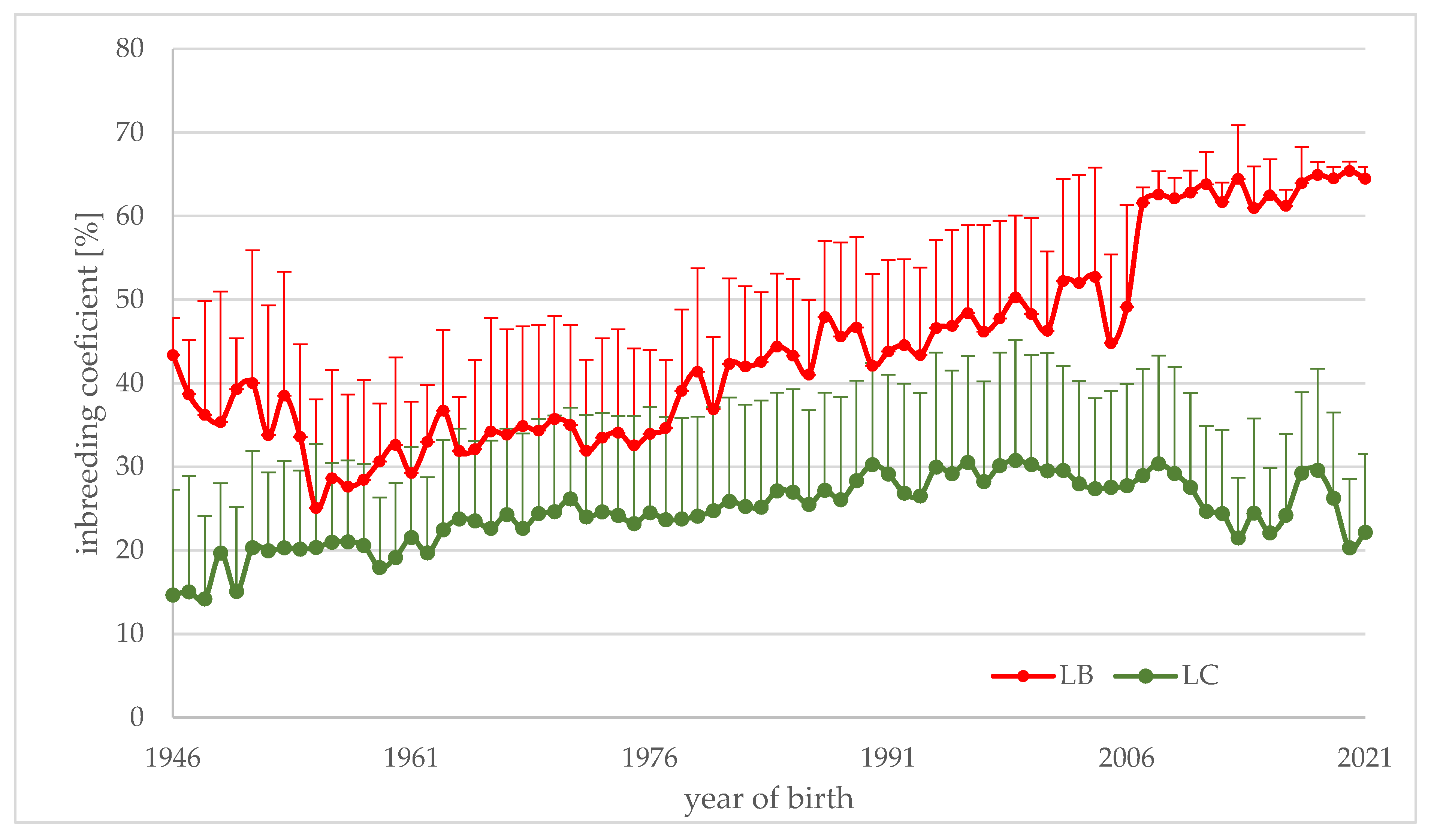
Table 2 presents the average values of the inbreeding coefficient for analyzed animals in the whole analyzed period of 75 years. There are significant differences between genetic lines but there is almost no difference between sexes and some differences between animals born in different seasons. The value of inbreeding is much higher within the LB line and is increasing much faster (Figure 1). For animals of the LB line born in the last year, their inbreeding is above 60%. In the LC line, inbreeding increased to the level of 30% twenty years ago, but, in recent years, the values were lower (Figure 1).
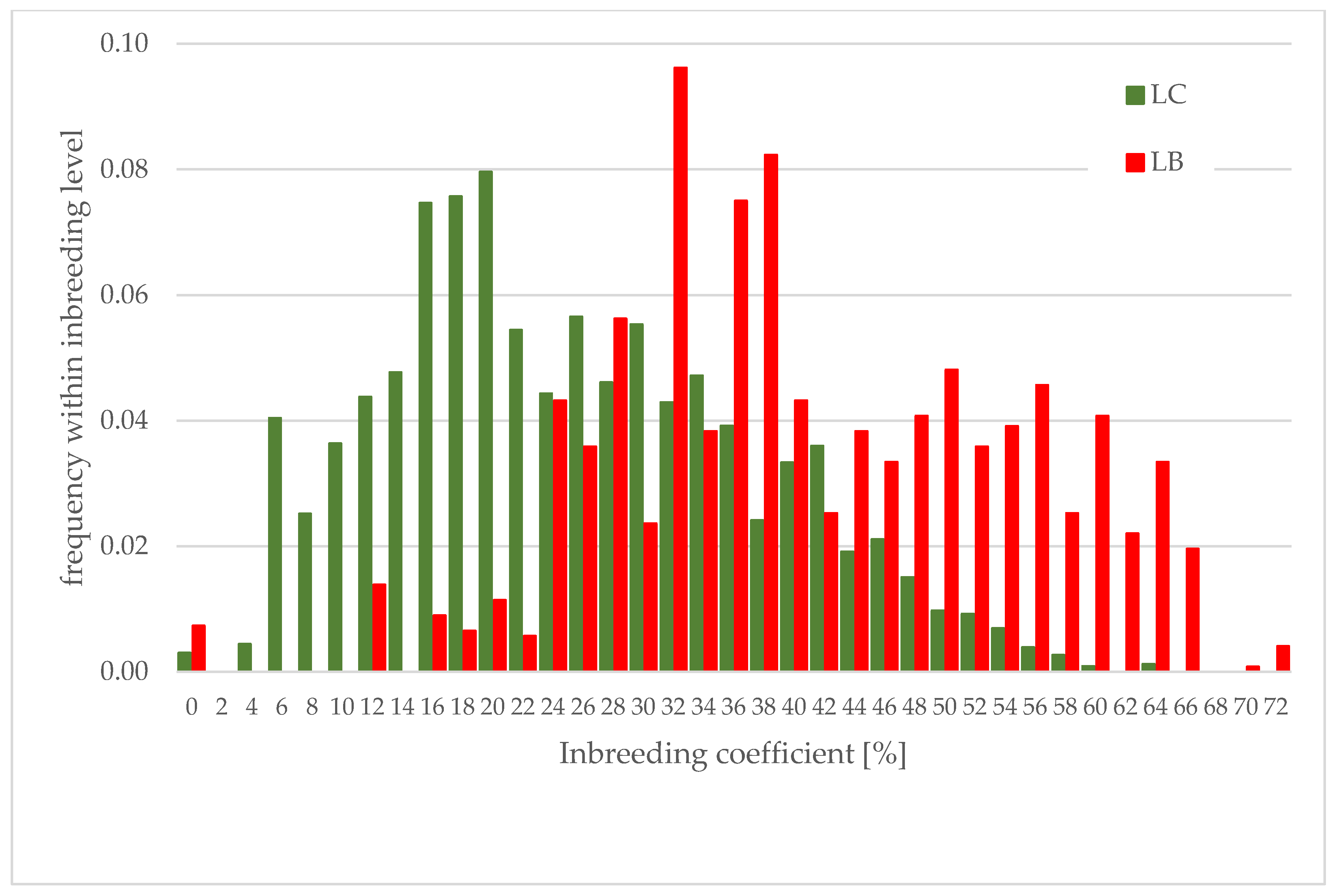
Figure 2 presents the distribution of the inbreeding coefficient for all analyzed European bison with known pedigree. Interesting are the differences between the distribution of inbreeding levels in both lines. In the LB line, there is a lack of values between 0 and 10%, and in the next few intervals, the proportion of animals is very low (Figure 2).
The influence of inbreeding, sex and season of birth on survival is presented in Table 3, Table 4 and Table 5.
In these three analyses, for all animals and separately for the LB and LC lines, there were no differences between males and females in survival rate, but there was a difference regarding the birth season. Animals born in the Spring season (April–July) had the largest survival rate in comparison to Winter (December–March). This provides additional proof that seasonality in reproduction is most profitable for animals.
The influence of the inbreeding coefficient upon the survival rate for the whole population is negative but not very large (EXP(B) = 0.590; p = 0.051), and close to slightly significant (Table 3). It could be explained that a completely inbred (F = 1) animal has almost half the chance for survival up to one month of age. However, the results in both lines are completely opposite. The value of the EXP(B) coefficient is very low for LC line animals (0.190) but very high for LB animals (6.569) and both are highly significant (Table 4). It could be explained that the survival rate for the fully inbred LC animals will be five times lower than for those with an inbreeding level equal to zero. However, within the LB line, the fully inbred animals have more than a six-times larger probability of surviving (Table 5).
4. Discussion
The two lines differ in inbreeding level as a consequence of the different number of founders. The average value for individuals from the LB line with a full known pedigree, born between 1946 and 2021, was larger than 0.410, but in the last twenty years, the average value was almost 0.60 (0.599) (Figure 1). The LC line is less inbred and its average value for the last 20 years was very similar to that for the whole 75 years (0.263 vs. 0.253) (Figure 1). In the last few years, the inbreeding coefficient within the LC line has been decreasing as a result of breeding recommendations. The recommendations for captive breeding were towards more even founders’ contributions and separation in breeding animals of the LC from the LB line [13,43,50]. A decrease in inbreeding level in the LC line was possible due to the much larger number of animals within this line.
There are other highly inbred species; for example, the median inbreeding coefficient for black robin (Petroica traversi) was equal to 0.34 and its maximal value was 0.54 [51]. This is similar to the median of the LB line (0.37) in this study, but larger than the median value in the LC line (0.23). The population of black robin was derived from a pair of founders, so the inbreeding level is constantly growing and this species is an example of the different direction of inbreeding’s influence on survival. Some rare breeds of domestic animals have similar inbreeding levels. For example, the Sorraia horse is derived from only 12 founders and the average inbreeding level in 2007 was equal to 0.325 ± 0.072 [52].
For other animal species in captivity, the inbreeding level is very different but rarely larger than 20% on average. The level of inbreeding in the small isolated moose (Alces alces) population in Norway was equal to 0.12 and 286/412 animals have an inbred coefficient larger than zero [53]. In a studied herd of red deer (Cervus elaphus), 42.1% of animals had inbreeding larger than zero and 20% had an inbreeding coefficient of 0.0625 and higher [54]. In an analyzed group of 15 species kept in zoos, the largest value of inbreeding was for the red-ruffed lemur (Varecia rubra), which was equal to 0.138, and for the African wolf (Lycaon pictus), at 0.108, and that for the rest of the species was much lower [55]. In an analysis of 88 animal species (119 populations), the level of inbreeding differed very significantly between analyzed populations. The mean inbreeding coefficient ranged from 0.015 for the Guam kingfisher (Todiramphus cinnamominus) to 0.352 for bharal (Pseudois nayaur) [37]. Data were collected from studbooks kept in zoos, so analyzed populations were rather small, but these values for some species are very similar to the values obtained for European bison. In the analyzed populations in zoos, the length of known pedigree (number of generations) or a small effective population size was connected with a higher inbreeding level. The Pere David deer (Elaphurus davidianus) was similar to European bison for some time, with only captive breeding and with the whole species derived from 11 founders, which caused high inbreeding, but no relation between the heterozygosity level and survival was found [56]. The Przewalski horse (Equus ferus przewalskii) also has a similar history, so the number of generations in the pedigree analysis was 6.86, and the mean inbreeding equaled 0.210 [37]. The pedigrees of European bison are very long and the calculation of the inbreeding coefficient was from the founding group. The number of generations included in this calculation averaged 7.43 and the maximum was equal to 15 generations from the founder. Thus, based on the pedigree, the European bison is one of the most inbred species, as an effect of the serious bottleneck and further isolation between breeding groups.
In the captive population of American bison (Bison bison), the average inbreeding coefficient was equal to 0.0326, but the share of animals with inbreeding larger than zero was only 14.43%, and fully traced generations were very low. The highest inbreeding coefficient found in this population was 0.4687. The Pedigree Book included data for a period longer than 100 years, but data about pedigree were not kept properly and the large number of gaps caused the underestimation of the inbreeding coefficient [57].
The influence of inbreeding upon survival is very common in studies about captive populations. Higher mortality of inbred offspring in zoo populations for 41 out of 44 tested mammal species was found [26]. In another work, offspring of related parents had, on average, a 33% lower survival rate [23]. Similarly, in the population of Canadian sheep (Ovis canadensis), it was found that the mortality of inbred individuals was 54%, compared to 22% for non-inbred animals [58]. In a meta-analysis, the influence of inbreeding for some species was estimated using the logistic model with only individual inbreeding. The values for 12 large herbivore species were significant, and for 11 of them, they were negative: between −5382 (muskox Ovibos moschatus) and −1.512 (Przewalski horse) [37]. The value for European bison presented in Table 3 was −0.527, but for the LC line, it was −1.658 (Table 4). The similarity between the Przewalski horse captive population and European bison was pointed out before. Both species passed a bottleneck and were, for a few generations, extinct in the wild, so their captive breeding was, and still is, very important.
In Pere David deer, the inbreeding depression on survival was not proven, but inbreeding was connected with higher susceptibility to multiple risks, such as high miscarriage rates, reduced life span and diseases [59]. In an analysis of 15 animal species kept in zoos, a negative relationship between inbreeding and survival for 13 species was found, while, for another two species, it was neutral [55].
Moreover, it is possible to point out some species in which the inbreeding relationship with survival is the opposite. For example, in Indian rhinoceros (Rhinoceros unicornis), inbred calves had a lower mortality rate (14%, n = 44) than non-inbred calves (22%, n = 126) [60].
Many authors, when checking the inbreeding depression’s effect on survival, consider in models not only their own inbreeding but also that of the mother or father or earlier ancestors. For the most inbred bird species (black robin), it was found that inbred chicks survived better when their mothers were inbred [51]. However, the results of other studies are different and maternal inbreeding does not have any influence. For example, the estimate of maternal inbreeding in a study on 15 zoos species varied from −0.0300 to 0.0341 and paternal inbreeding from 0.0237 to 0.0409, but, at the same time, individual inbreeding has a negative influence, with the value of the regression coefficient from −0.1940 to −0.1323 [55]. For Indian rhinoceros, it was shown that neither zoo generation (p = 0.193) nor inbreeding of the mother (p = 0.626) influenced infant mortality [60]. In the analyzed population of European bison, the level of inbreeding of the mother and her progeny was correlated, so this is the reason that inbreeding of the mother was not included in the model.
The results for 119 populations in captivity show that mainly individual inbreeding has a negative effect upon survival, but some analyses present species or populations in which the relationship is the opposite [37]. Such is the case for the LB line of European bison, where survival is positively correlated with inbreeding. It is possible to notice the lack of small values in the distribution of the inbreeding coefficient in the LB line (Figure 2). This could be a result of common matings between closely related animals at the beginning of the restitution. For example, one captive breeding herd in Pszczyna started in 1865, with four animals, and the inbreeding in such a herd was certainly not zero at the beginning of the XX century [61].
Such exceptions where the relation between inbreeding and survival is positive are sometimes considered as the effect of purging [33]. Inbred animals surviving to reproductive age are less likely to carry deleterious alleles than non-inbred animals. Templeton and Read [62] reported that inbreeding depression was lower in offspring born to selected inbred parents than it was prior to the selection program. Based on these results, this “purging” strategy has been recommended for use in captive populations suffering from severe inbreeding depression [12,33,62].
In the European bison population, the difference between the two lines is very interesting and the various numbers of founders explain the difference in the level of inbreeding. In both lines, the inbreeding was growing—faster in the LB line than the LC line. In the LB line, there should be a larger negative effect of inbreeding, but there is not [11,19,21]. The reason for this could be explained by the purging in the beginning of the restitution period, when the inbreeding of LB line animals grew very rapidly, and this made it possible for this line to eliminate deleterious alleles. According to some authors, purging occurs when inbreeding is growing slowly [33]. However, on the other hand, if the selection against recessive alleles is taken into consideration, it would be much more effective with a fast increase in inbreeding. This could be the explanation for the obtained results for the LB line of European bison. The LC line is typical for the majority of analyzed populations.
5. Conclusions
- The European bison, in comparison with other species, is very highly inbred. For animals with a fully known pedigree born in years 1946–2021, the average value of the inbreeding coefficient varies between lines: in the LB line, it is equal to 0.419, and in the LC line, it is 0.253, which is the effect of the different numbers of founders.
- Survival up to one month is negatively influenced by inbreeding only for animals belonging to the LC line. In the LB line, the relation is the opposite, probably as a result of purging in the period of the beginning of the restitution.
- The study of inbreeding and its relation with fitness should be continued.
Funding
This research was partly funded by the Forest Fund (Poland), grant number OR.271.3.10.2017.
Institutional Review Board Statement
Not applicable.
Data Availability Statement
All data are available on the webpage of European Bison Pedigree Book at URL (accessed on 20 December 2022): https://bpn.com.pl/index.php?option=com_content&task=view&id=1133&Itemid=213.
Acknowledgments
I am grateful to my colleagues for all comments and corrections. I thank Julia and Katherine Rossi for the kind improvement of the English. I also thank for comments from three anonymous reviewers and editors what have substantially improved the manuscript.
Conflicts of Interest
The author declares no conflict of interest.
References
- Raczyński, J. European Bison; PWRiL: Warszawa, Poland, 1978; pp. 1–246. (In Polish) [Google Scholar]
- Pucek, Z. History of the European bison and problems of its protection and management. In Global Trends in Wildlife Management; Bobek, B., Perzanowski, K., Regelin, W., Eds.; Swiat Press: Krakow-Warszawa, Poland, 1991; pp. 19–39. [Google Scholar]
- von der Groeben, G. Das Zuchtbuch. In Berichte Internationale, Geselschaft zur Erhaltung des Wisents; Kommission bei Dr W. Stichel: Leipzig, Germany, 1932; pp. 5–50. [Google Scholar]
- Raczyński, J.; Bołbot, M. European Bison Pedigree Book 2021; Białowieski National Park: Białowieża, Poland, 2022; pp. 1–80. [Google Scholar]
- Slatis, H.M. An analysis of inbreeding in the European bison. Genetics 1960, 45, 275–287. [Google Scholar] [CrossRef] [PubMed]
- Olech, W. The number of ancestors and their contribution to European bison (Bison bonasus L.) population. Ann. Wars. Agric. Univ. Anim. Sci. 1999, 35, 111–117. [Google Scholar]
- Olech, W. The changes of founders’ numbers and their contribution to the European bison population during 80 years of species’ restitution. Eur. Bison Conserv. Newsl. 2009, 2, 54–60. [Google Scholar]
- Olech, W. The participation of ancestral genes in the existing population of European bison. Acta Theriol. 1989, 34, 397–407. [Google Scholar] [CrossRef] [Green Version]
- Olech, W. The analysis of European bison genetic diversity using pedigree data. In Health Threats for the European Bison Particularly in Free-Roaming Populations in Poland; Kita, J., Anusz, K., Eds.; The SGGW Publishers: Warszawa, Poland, 2006; pp. 205–236. [Google Scholar]
- Parusel, J.B. European bison from Pszczyna and their role in species restitution. Eur. Bison Conserv. Newsl. 2009, 2, 129–136. (In Polish) [Google Scholar]
- Olech, W. Analysis of inbreeding in European bison. Acta Theriol. 1987, 32, 373–387. [Google Scholar] [CrossRef] [Green Version]
- Ballou, J.D. Ancestral inbreeding only minimally affects inbreeding depression in mammalian populations. J. Hered. 1997, 88, 169–178. [Google Scholar] [CrossRef]
- Pucek, Z.; Belousova, I.P.; Krasińska, M.; Krasiński, Z.A.; Olech, W. European Bison Status Survey and Conservation Action Plan; IUCN The World Conservation Union: Gland, Switzerland, 2004; pp. 1–49. [Google Scholar]
- Matuszewska, M.; Olech, W.; Bielecki, W.; Osińska, B. The influence of inbreeding into pathological changes occurrence in European bison males reproduction tract. Park. Nar. Rezerw. Przyr. Polsce 2004, 23, 679–685. (In Polish) [Google Scholar]
- Sobieraj, A.; Olech, W. Twenty years of the European bison Lowland line Bison bonasus bonasus conservation in captivity. Ann. WULS—Anim. Sci. 2018, 57, 171–182. [Google Scholar] [CrossRef]
- Johnson, H.E.; Mills, L.S.; Wehausen, J.D.; Stephenson, T.R.; Luikart, G. Translating effects of inbreeding depression on component vital rates to overall population growth in endangered bighorn sheep. Conserv. Biol. 2011, 25, 1240–1249. [Google Scholar] [CrossRef]
- Reed, T.E.; Grotan, V.; Jenouvrier, S.; Saether, B.-E.; Visser, M.E. Population growth in a wild bird is buffered against phenological mismatch. Science 2013, 340, 488–491. [Google Scholar] [CrossRef] [PubMed]
- Belousova, I.P.; Smirnov, K.A.; Kasmin, V.D.; Kudryavtsev, I.V. Genetic characteristics and prognosis for existence of the European bison free-living population created in the Orlovskoe Poles’e National Park. Russ. J. Genet. 2004, 40, 295–299. [Google Scholar] [CrossRef]
- Olech, W. The Influence of Individual and Maternal Inbreeding on the Survival of European Bison Calves; Warsaw University of Life Sciences: Warsaw, Poland, 2003; pp. 1–78. (In Polish) [Google Scholar]
- Olech, W. The influence of inbreeding on European bison sex ratio. In Animals, Zoos and Conservation; Zgrabczyńska, E., Ćwiertnia, P., Ziomek, J., Eds.; Life Sicience University: Poznań, Poland, 2006; pp. 29–33. [Google Scholar]
- Kobryńczuk, F. The influence of inbreeding on the shape and size of the skeleton of the European bison. Acta Theriol. 1985, 30, 379–422. [Google Scholar] [CrossRef] [Green Version]
- Gill, J. The Physiology of European Bison; Severus: Warszawa, Poland, 1999; pp. 1–176. (In Polish) [Google Scholar]
- Ralls, K.; Ballou, J.D.; Templeton, A. Estimates of lethal equivalents and the cost of inbreeding in mammals. Conserv. Biol. 1988, 2, 185–193. [Google Scholar] [CrossRef]
- Ralls, K.; Brugger, K.; Ballou, J. Inbreeding and juvenile mortality in small populations of ungulates. Science 1979, 206, 1101–1103. [Google Scholar] [CrossRef]
- Frankham, R.; Ballou, J.D.; Briscoe, D.A. Introduction to Conservation Genetics; Cambridge University Press: Cambridge, UK, 2002; pp. 1–140. [Google Scholar]
- Ralls, K.; Ballou, J. Effects of inbreeding on juvenile mortality in some small mammal species. Lab. Anim. 1982, 16, 159–166. [Google Scholar] [CrossRef] [Green Version]
- Frankham, R.; Ralls, K. Inbreeding leads to extinction. Nature 1998, 392, 441–442. [Google Scholar] [CrossRef]
- Saccheri, I.; Kuussaari, M.; Kankare, M.; Vikman, P.; Fortellus, W.; Hanski, I. Inbreeding and extinction in a butterfly metapopulation. Nature 1998, 392, 491–494. [Google Scholar] [CrossRef]
- Laikre, L. Hereditary effects and conservation genetic management of captive population. Zoo Biol. 1999, 18, 81–99. [Google Scholar] [CrossRef]
- Bouwmeester, J.; Mulder, J.L.; van Bree, P.H.J. High incidence of malocclusion in an isolated population of the red fox (Vulpes vulpes) in the Netherland. J. Zool. 1989, 219, 123–136. [Google Scholar] [CrossRef]
- Pemberton, J. Measuring inbreeding depression in the wild: The old ways are the best. Trends Ecol. Evol. 2004, 19, 613–615. [Google Scholar] [CrossRef]
- Slate, J.; Kruuk, L.E.B.; Marshall, T.C.; Pemberton, J.M.; Clutton-Brock, T.H. Inbreeding depression influences lifetime breeding success in a wild population of red deer (Cervus elaphus). Proc. R. Soc. Lond. B 2000, 267, 1657–1662. [Google Scholar] [CrossRef] [PubMed] [Green Version]
- Hedrick, P.H.; Garcia-Dorado, A. Understanding inbreeding depression, purging and genetic rescue. Trends Ecol. Evol. 2016, 31, 940–952. [Google Scholar] [CrossRef] [PubMed]
- Ballou, J.D.; Lacy, R.C. Identifying genetically important individuals for management of genetic diversity in pedigreed populations. In Population Management for Survival and Recovery; Ballou, J.D., Foose, T.J., Gilpin, M.E., Eds.; Columbia University Press: New York, NY, USA, 1995; pp. 76–111. [Google Scholar]
- Byers, D.L.; Waller, D.M. Do plant populations purge their genetic load? Effects of population size and mating history on inbreeding depression. Annu. Rev. Ecol. Syst. 1999, 30, 479–513. [Google Scholar] [CrossRef] [Green Version]
- Crnokrak, P.; Barrett, S.C.D. Perspective: Purging the genetic load: A review of the experimental evidence. Evolution 2002, 56, 2347–2358. [Google Scholar] [PubMed]
- Boakes, E.H.; Wang, J.; Amos, W. An investigation of inbreeding depression and purging in captive pedigreed populations. Heredity 2007, 98, 172–182. [Google Scholar] [CrossRef] [Green Version]
- Kalinowski, S.T.; Hedrick, P.W.; Miller, P.S. No inbreeding depression observed in Mexican and red wolf captive breeding programs. Conserv. Biol. 1999, 13, 1371–1377. [Google Scholar] [CrossRef]
- Bouzat, J.l. Conservation genetics of population bottlenecks: The role of chance, selection, and history. Conserv. Genet. 2010, 11, 463–478. [Google Scholar] [CrossRef]
- López-Cortegano, E.; Moreno, E.; García-Dorado, A. Genetic purging in captive endangered ungulates with extremely low effective population sizes. Heredity 2021, 127, 433–442. [Google Scholar] [CrossRef] [PubMed]
- Carr, D.E.; Dudash, M. Recent approaches into the genetic basis of inbreeding depression in plants. Philos. Trans. R. Soc. Lond. B 2003, 358, 1071–1084. [Google Scholar] [CrossRef]
- Wang, J.; Hill, W.G.; Charlesworth, D.; Charlesworth, B. Dynamics of inbreeding depression due to deleterious mutations in small populations: I. Mutation parameters and inbreeding rate. Genet. Res. 1999, 74, 165–178. [Google Scholar] [CrossRef] [PubMed]
- Krasińska, M.; Krasiński, Z.A.; Perzanowski, K.; Olech, W. European bison Bison bonasus (Linnaeus, 1758). In Ecology, Evolution and Behaviour of Wild Cattle: Implications for Conservation; Melleti, M., Burton, J., Eds.; Cambridge University Press: Cambridge, UK, 2014; pp. 115–173. [Google Scholar]
- Krasiński, Z. The restitution of European bison in Białowieża in years 1929–1952. Park. Nar. Rezerw. Przyr. 1994, 4, 3–23. (In Polish) [Google Scholar]
- Kaczmarek-Okrój, M.; Olech, W. Reproduction parameters of wisent in ex situ condition. Eur. Bison Conserv. Newsl. 2022, 14, 29–42. [Google Scholar]
- Krasiński, Z.; Raczyński, J. The reproduction biology of European bison living in reserves and in freedom. Acta Theriol. 1967, 29, 407–444. [Google Scholar] [CrossRef] [Green Version]
- EBPB—European Bison Pedigree Book; URL. 1133. Available online: https://bpn.com.pl/index.php?option=com_content&task=view&id=1133&Itemid=213 (accessed on 20 December 2022).
- Olech, W.; Michalska, E. Comparison of inbreeding in two closed herd. Zwierz. Lab. 1999, 27, 3–8. [Google Scholar]
- Quaas, R.L. Computing the diagonal elements and inverse of a large numerator relationship matrix. Biometrics 1976, 32, 949–953. [Google Scholar] [CrossRef]
- Olech, W.; Perzanowski, K. (Eds.) European Bison (Bison bonasus) Strategic Species Status Review 2020; IUCN SSC Bison Specialist Group and European Bison Conservation Center, European Bison Friends Society: Warsaw, Poland, 2022; pp. 1–138. [Google Scholar]
- Weiser, E.L.; Grueber, C.E.; Kennedy, E.S.; Jamieson, I.G. Unexpected positive and negative effects of continuing inbreeding in one of the world”s most inbred wild animals. Evolution 2015, 70, 154–166. [Google Scholar] [CrossRef] [PubMed]
- Luis, C.; Cothran, E.G.; do Mar Oomm, M. Inbreeding and Genetic Structure in the Endangered Sorraia Horse Breed: Implications for its Conservation and Management. J. Hered. 2007, 98, 232–237. [Google Scholar] [CrossRef]
- Haanes, H.; Markussen, S.S.; Herfindal, I.; Røed, K.H.; Solberg, E.J.; Heim, M.; Midthjell, L.; Sæther, B.E. Effects of inbreeding on fitness-related traits in a small isolated moose population. Ecol. Evol. 2013, 3, 4230–4242. [Google Scholar] [CrossRef]
- Walling, C.A.; Nussey, D.H.; Morris, A.; Clutton-Brock, T.H.; Kruuk, L.E.B.; Pemberton, J.M. Inbreeding depression in red deer calves. Evol. Biol. 2011, 11, 318. [Google Scholar] [CrossRef] [PubMed] [Green Version]
- Farquharson, K.A.; Hogg, C.J.; Grueber, C.E. Offspring survival changes over generations of captive breeding. Nat. Commun. 2021, 12, 3045. [Google Scholar] [CrossRef]
- Zeng, Y.; Li, C.; Zhang, L.; Zhong, Z.; Jiang, Z. No correlation between neonatal fitness and heterozygosity in a reintroduced population of Père David’s deer. Curr. Zool. 2013, 59, 249–256. [Google Scholar] [CrossRef]
- Skotarczak, E.; Ćwiertnia, P.; Szwaczkowski, T. Pedigree structure of American bison (Bison bison) population. Czech J. Anim. Sci. 2018, 63, 507–517. [Google Scholar] [CrossRef] [Green Version]
- Sausman, K.A. Survival of captive born Ovis canadensis in North American zoos. Zoo Biol. 1984, 3, 111–121. [Google Scholar] [CrossRef]
- Zhang, S.; Li, C.; Li, Y.; Chen, Q.; Hu, D.; Cheng, Z.; Wang, X.; Shan, Y.; Bai, J.; Liu, G. Genetic differentiation of reintroduced Père David’s deer (Elaphurus davidianus) based on population genomics analysis. Front Genet. 2021, 12, 705337. [Google Scholar] [CrossRef]
- Zchokke, S.; Baur, B. Inbreeding, outbreeding, infant growth and size dimorphism in captive Indian rhinoceros. Can. J. Zool. 2002, 80, 2014–2023. [Google Scholar] [CrossRef] [Green Version]
- Parusel, J.B. If it had not been for the European bison of Pszczyna…. Eur. Bison Conserv. Newsl. 2019, 12, 69–78. (In Polish) [Google Scholar]
- Templeton, R.A.; Read, B. Elimination of inbreeding depression from a captive populations of Speke’s gazelle. Validity of original statistical analysis and confirmation by permutation testing. Zoo Biol. 1998, 17, 77–94. [Google Scholar] [CrossRef]
Figure 1.
The mean inbreeding coefficient with standard deviation bar for animals of LB and LC lines with full known pedigree born in years 1946–2021.
Figure 1.
The mean inbreeding coefficient with standard deviation bar for animals of LB and LC lines with full known pedigree born in years 1946–2021.

Figure 2.
The distribution of inbreeding coefficient within both genetic lines for all animals with known pedigree. Values of inbreeding coefficient were divided into intervals of 2%.
Figure 2.
The distribution of inbreeding coefficient within both genetic lines for all animals with known pedigree. Values of inbreeding coefficient were divided into intervals of 2%.


Table 1.
The number of European bison registered in EBPB up to 2021 and analyzed with information about survival to first month of age and the proportion of males.
Table 1.
The number of European bison registered in EBPB up to 2021 and analyzed with information about survival to first month of age and the proportion of males.
| Group | Number | Survival to First Month | Males | ||
|---|---|---|---|---|---|
| Number | % | Number | % | ||
| Global population: all registered born until 2021 | 13,750 | 12,404 | 90.2 | 6716 | 48.8 |
| Line LC * | 9801 | 8778 | 89.6 | 4874 | 49.7 |
| Line LB * | 3949 | 3627 | 91.8 | 1842 | 46.6 |
| Analyzed: (with full known pedigree and born 1946–2021) | 6868 | 6051 | 88.1 | 3435 | 50.0 |
| Line LC | 5641 | 4943 | 87.6 | 2849 | 50.5 |
| Line LB | 1227 | 1108 | 90.3 | 586 | 47.8 |
* LC—Lowland-Caucasian line; LB—Lowland line.
Table 2.
Mean values of inbreeding coefficient of analyzed animals (with known pedigree and born in 1946–2021) divided into genetic lines.
Table 2.
Mean values of inbreeding coefficient of analyzed animals (with known pedigree and born in 1946–2021) divided into genetic lines.
| Line LC | Line LB | Both Lines Together | ||||||
|---|---|---|---|---|---|---|---|---|
| Number | Average | s.d. | Number | Average | s.d. | Average | s.d. | |
| All analyzed animals | 5641 | 0.253 | 0.121 | 1227 | 0.410 | 0.136 | 0.281 | 0.137 |
| F | 2792 | 0.257 | 0.122 | 641 | 0.402 | 0.136 | 0.284 | 0.137 |
| M | 2849 | 0.250 | 0.119 | 586 | 0.419 | 0.135 | 0.279 | 0.137 |
| not surviving until 1st month | 698 | 0.276 | 0.127 | 119 | 0.379 | 0.124 | 0.291 | 0.132 |
| surviving to 1st month | 4943 | 0.250 | 0.119 | 1108 | 0.413 | 0.136 | 0.280 | 0.138 |
| born in Spring | 3546 | 0.248 | 0.119 | 857 | 0.410 | 0.136 | 0.280 | 0.139 |
| born in Autumn | 1776 | 0.260 | 0.121 | 335 | 0.408 | 0.136 | 0.283 | 0.134 |
| born in Winter | 244 | 0.287 | 0.132 | 32 | 0.415 | 0.145 | 0.302 | 0.139 |
Seasons: Spring (April–July); Autumn (August–November); Winter (December–March).
Table 3.
The relationship between the sex, birth season and inbreeding level, and survival to the age of one month for all analyzed animals born between 1946 and 2021 with known pedigree. Males within sex and Winter within season were reference levels, with B value equal to zero.
Table 3.
The relationship between the sex, birth season and inbreeding level, and survival to the age of one month for all analyzed animals born between 1946 and 2021 with known pedigree. Males within sex and Winter within season were reference levels, with B value equal to zero.
| Source | B * | Standard Error | Wald χ2 * | p Value | Exp (B) * |
|---|---|---|---|---|---|
| Intercept | 1.211 | 0.1643 | 54.289 | 0.000 | 3.356 |
| Sex—Female | 0.021 | 0.0749 | 0.075 | 0.784 | 1.021 |
| Season—Spring | 0.992 | 0.1459 | 46.264 | 0.000 | 2.698 |
| Season—Autumn | 0.938 | 0.1534 | 37.365 | 0.000 | 2.555 |
| Inbreeding coefficient | −0.527 | 0.2696 | 3.820 | 0.051 | 0.590 |
* B—regression coefficient; EXP(B); EXP(B)—Euler number to the power of B; Wald χ2—the Chi-square test to check the significance of the source values.
Table 4.
The relationship between the sex, birth season and inbreeding level, and survival to the age of one month, of European bison belonging to LC line born between 1946 and 2021 with known pedigree. Males within sex and Winter within season were reference levels, with B value equal to zero.
Table 4.
The relationship between the sex, birth season and inbreeding level, and survival to the age of one month, of European bison belonging to LC line born between 1946 and 2021 with known pedigree. Males within sex and Winter within season were reference levels, with B value equal to zero.
| Source | B * | Standard Error | Wald χ2 | p Value | Exp (B) * |
|---|---|---|---|---|---|
| Intercept | 1.477 | 0.1796 | 67.638 | 0.000 | 4.380 |
| Sex—Female | 0.046 | 0.0816 | 0.320 | 0.572 | 1.047 |
| Season—Spring | 0.923 | 0.1549 | 35.490 | 0.000 | 2.516 |
| Season—Autumn | 0.961 | 0.1633 | 34.645 | 0.000 | 2.615 |
| Inbreeding coefficient | −1.658 | 0.3299 | 25.268 | 0.000 | 0.190 |
* explained below Table 3.
Table 5.
The relationship between the sex, birth season and inbreeding level, and survival to the age of one month, of European bison belonging to LB line born between 1946 and 2021 with known pedigree. Males within sex and Winter within season were reference levels, with B value equal to zero.
Table 5.
The relationship between the sex, birth season and inbreeding level, and survival to the age of one month, of European bison belonging to LB line born between 1946 and 2021 with known pedigree. Males within sex and Winter within season were reference levels, with B value equal to zero.
| Source | B * | Standard Error | Wald χ2 | p Value | Exp (B) * |
|---|---|---|---|---|---|
| Intercept | 0.733 | 0.546 | 1.803 | 0.179 | 2.081 |
| Sex—Female | −0.054 | 0.195 | 0.078 | 0.780 | 0.947 |
| Season—Spring | 0.940 | 0.4722 | 3.964 | 0.046 | 2.560 |
| Season—Autumn | 0.522 | 0.4853 | 1.157 | 0.282 | 1.685 |
| Inbreeding coefficient | 1.882 | 0.7222 | 6.793 | 0.009 | 6.569 |
* explained below Table 3.
Disclaimer/Publisher’s Note: The statements, opinions and data contained in all publications are solely those of the individual author(s) and contributor(s) and not of MDPI and/or the editor(s). MDPI and/or the editor(s) disclaim responsibility for any injury to people or property resulting from any ideas, methods, instructions or products referred to in the content. |
© 2023 by the author. Licensee MDPI, Basel, Switzerland. This article is an open access article distributed under the terms and conditions of the Creative Commons Attribution (CC BY) license (https://creativecommons.org/licenses/by/4.0/).
Share and Cite
MDPI and ACS Style
Olech, W. The Relationship between Inbreeding and Fitness Is Different between Two Genetic Lines of European Bison. Diversity 2023, 15, 368. https://doi.org/10.3390/d15030368
AMA Style
Olech W. The Relationship between Inbreeding and Fitness Is Different between Two Genetic Lines of European Bison. Diversity. 2023; 15(3):368. https://doi.org/10.3390/d15030368
Chicago/Turabian StyleOlech, Wanda. 2023. "The Relationship between Inbreeding and Fitness Is Different between Two Genetic Lines of European Bison" Diversity 15, no. 3: 368. https://doi.org/10.3390/d15030368
Note that from the first issue of 2016, this journal uses article numbers instead of page numbers. See further details here.