1. Introduction
Because the wood of trees is a long-lived—comparably to human life—material, it has been considered since long ago to be a natural archive of environmental records. The growth of tree rings is quite an elaborated research area. The process of transforming a cambium cell into a mature xylem cell is largely known, and the approaches to successful modeling of the process have been developed [
1].
Variations of contemporary or paleoclimate as well as variations in environmental chemistry belong to the records that can be obtained and analyzed. Within the area of environmental chemistry, studies of anomalies of element concentration in tree rings have been developing since the 1970s–80s. The anomalies were attributed to the modern development of industry emitting various pollutants [
2,
3,
4,
5,
6,
7,
8], alterations of soil chemistry due to fertilization [
9], ancient volcano eruptions [
10,
11,
12], or general stress [
13].
Measurements of elemental content across tree rings produce data series revealing long-term patterns of element deposition in the wood. It has been shown [
13] that some elements (Mn, Zn) displayed falling concentration trends in the wood of a number of tree species whereas others (Rb) stayed at quite stable concentrations from the pith of the stem and outward.
The studies of such trends may be of importance because they help to evaluate inferences from the data series analysis. In the wood of
Pinus ponderosa Douglas ex C. Lawson, Padilla and Anderson [
14] found that Sr, Ba, Zn, and Cd displayed an uprising trend in the early 1800s which lasted for approximately 50 years; then the element’s concentration decreased up to 2000s. In other studies reviewed by Padilla and Anderson [
14], similar dynamics in Ca, Mg, and Zn were attributed to acid rains. However, the research area of Padilla and Anderson did not have any record of anthropogenic acid rains and thus, as was concluded by the authors, the long element trends could not be explained by the exposure to acid rains.
Significantly, trends of some elements can correlate with each other whereas being uncorrelated with other elemental trends. Goldberg et al. [
15] have reported the analysis of elements in cores of Siberian larch. They divided all the studied elements into two groups. The first group comprised Br, Zn, and Cl, and the second one included K, Ca, Sr, Mn, and Fe. The difference between the elements of the groups was that the first group elemental trends reflected the precipitation variations throughout the whole time of analysis while the elements of the second group concentrated mainly in the outer part of the stem.
Because of the physically the same measurement objects—tree rings—the dendrochemistry area is often considered to be a part of dendrochronology. And as such, dendrochemistry inherited from the latter many methodological approaches. In particular, a single core extracted from a tree stem often serves as a reliable representative of the growth pattern of that stem. The basis of the reliability is the possibility to use various chronologies built previously for local areas, which helps to recognize defects in the series of tree rings.
Unfortunately, what concerns dendrochemistry, quite a number of confounding factors may obscure the relationships of wood chemistry with environmental parameters. The content and concentrations of inorganics in wood vary widely both within and between species [
16].
Though many details regarding the distribution of chemical elements in tree rings have been established [
17,
18,
19], it is little known how tightly the elements attach to the xylem matrix. Research on how movable the elements are in the xylem, both radially and tangentially, often gives controversial results [
20]. There is, therefore, much less confidence regarding whether a single core analyzed for elemental distribution may surely represent the distribution in the entire tree stem. The importance of such knowledge cannot be overrated. The distribution of elements in the wood of trees is used not only for detecting ancient eruptions, which satisfies mostly academic interests. The elemental content of tree rings is accepted as a source of evidence in courts during legal actions against industrial companies [
21,
22].
Thus, the purposes of the study were (i) to estimate the radial variability of the element’s distribution across the stems in a worldwide represented species of Scots pine (Pinus sylvestris L.) and (ii) to estimate whether the element distribution in one core correlates with that in another core.
2. Materials and Methods
2.1. Area of Research
Figure 1 depicts the geographical location of the study area. The sampling site has been found in the suburb of Krasnoyarsk city, in a large, forested area which has GPS coordinates 55°59′29.94″ N and 92°42′19.12″ E. The area is covered by a Scots pine forest of around 100 years old, with an admixture of birch, aspen, and Siberian larch. A gentle slope on the left bank of the Yenissei River is south-oriented and has a.s.l. values of 280 to 300 m.
The parent rock is represented by volcanic rocks of the basic composition. According to the World reference base (WRB) for soils 2014, the soil type is Albic Luvisols, profile Ah(0-8)-Bt(9-20)-Ck(21-70). In the soil, the concentration of fine clay minerals (fraction < 0.01 mm) varies between 2% and 17% as measured after the Kaczynski method. Organic C content (after the Tyurin method) varied in the range of 1–7%. The pH value varied from 5.81 to 8.26 in the soil. The amount of Fe2O3 increases down the profile. The cation exchange capacity (CEC) decreases down the profile, from 36.25 mEq/100 g in the humus horizon to 2.2 mEq/100 g in the parent rock.
2.2. Sampling
The sampling of trees took place in October 2020 (after the cessation of the seasonal growth) and in April 2021 (before the onset of the growth). For the sampling, apparently healthy trees of visually similar sizes have been chosen. At every tree, the sides of the stem facing north, south, west, and east have been found with the help of a compass. After that, the 12 mm cores have been extracted with the help of a Haglof borer at the height of 1 to 1.2 m from the ground, four cores per tree, corresponding to the cardinal directions (
Figure 2). Altogether, six trees and 24 cores have been sampled. For the purpose of the analysis, the trees are numbered from #1 to #6.
After the sampling, the cores were wrapped into a firm paper, marked, and transported to the laboratory where they were air-dried before further treatment.
2.3. Scanning for Elements
From all the cores, 2 mm slices were sawn perpendicular to the wood grains with the help of a circular saw. The slices were scanned with Itrax Multiscanner (COX Analytical Systems, Sweden, 2012) coupled with Multi Scanner Navigator software 6.5.3.
Itrax Multi Scanner is a scanner with a thin X-ray beam. The facility design is based on polyplane capillary optics Cox which generates a beam from an X-ray tube as a rectangle of 20 mm by 50 µm. The characteristic X-ray radiation is registered by a Si-based detector SDD (Ketek GmbH, München, Germany) which has a resolution of 140 eV at 5.9 keV and can register up to 200,000 photons a second (cps). The collimating optics in SDD limits the radiation registration by a square of 0.05 mm by 2 mm. The spatial resolution of scanning was 100 µm. The analysis of light elements at an acceptable detection limit is performed through an X-ray tube with a Cr anode (1.9 kWt). For Ti and heavier elements, an X-ray tube with Mo anode (3 kWt) is used. For an optimal relation of the useful signal and the background, the dwelling time amounts to 10 s a point. For wood samples, the optimal voltage and amperage are 50 kV and 30 mA, correspondingly.
Altogether, 13 chemical elements were monitored in the research. They are Al, Si, P, S, Cl, K, Ca, Ti, Mn, Fe, Cu, Zn, and Sr. Most of the elements are either biologically active or may be biologically active.
For each element, the multi-scanner produces a long series of data which are relative units (counts per second) theoretically related to the number of the element nuclei contained in the point of scanning.
2.4. Data Analysis
According to the time of sampling, the outermost tree ring was dated 2020. The tree rings had quite well-recognizable borders, especially on X-ray density images, and thus we were able to follow the elemental counts up to 1940, in most of the cases. So, the series of tree rings to study were 81 years long, with one exclusion due to damage to the core.
The wooden slices have a variable physical density along the scanning path. Theoretically, the variations in the density may affect the measured counts of the elements. To compensate for the variations, normalizing may be used. In the method, the density of the specimen is reflected in the parameter of incoherent radiation (IR) which is provided by the facility for every scanning point along with the counts. Therefore, all the elemental counts for individual points were divided by a normalizing coefficient (NC) which is NC = IR/AIR, where AIR is the average IR for the studied series of tree rings.
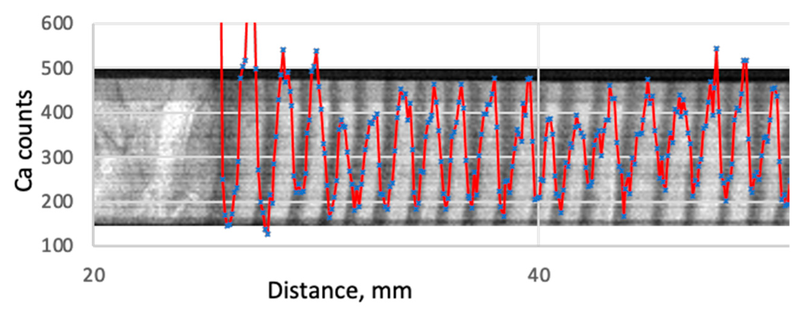
Because the widths of tree rings vary, the number of scanning points falling within the rings differs. This means that the number of elemental counts will tend to be higher in wider rings, which makes them incomparable. To compare the rings regarding the elemental content we adopted an approach to calculate a relative value, namely, an average number of counts per one scanning point within a ring, as follows.
First, the core is divided into a series of scanning points, the borders of the series being the outer borders of tree rings seen on the X-ray density image (
Figure 3). Second, all the counts within the ring—for a definite element—are summed up and divided by the number of scanning points. The resultant value is the average number of counts per scanning point for the particular tree ring.
To solve the task of the study, correlation analysis has been applied. It is well known that the parametrical correlation methods are only applicable when the sample data are normally distributed. However, when the data are numerous enough the condition of the normality is largely loosed. In this study, the length of the series was mostly 81 years. Thus, the standard Pearson correlation coefficient was adopted as the basic tool for the analysis.
The logic in the application of the correlation analysis was as follows. First, the distribution of elemental concentrations may be uniform around the circle and sufficiently vary across the rings, as, e.g., in
Figure 4a. In this case, one can expect a high positive correlation between radial sample cores. Second, the distribution may be irregular around the circle and sufficiently variable across the rings, as in
Figure 4b. In this case, one can expect a low, sometimes maybe negative, correlation between the radial directions. Third, the distribution may be uniform around the circle but be next to constant across the rings (
Figure 4c). In this case, one can also expect a low, close to zero, correlation. Lastly, the distribution may be uniform around the circle and vary sufficiently across the rings but not randomly, e.g., as a long trend (
Figure 4d). In the last case, a positive correlation may be expected.
The intra-tree correlations were estimated by calculations of Pearson’s correlation coefficients with the help of standard functions of R. In case of need, a detrending has been applied. The ARSTAN 49v1_Mac software (by Dr. Edward R. Cook, Columbia University, NY USA, and Paul J. Krusic, University of Cambridge, UK) has been used for the detrending, with the detrending options being the Hugershof curve and a smoothing spline. Also, the detrending in the form of differences between neighboring values (a discreet analog of the derivative) has been used. The derivative detrending was formally presented as:
where
x represents the initial series,
x* is the detrended series, and
t is the year as per tree rings.
3. Results
The received correlation matrices are too big, so, they are presented in
Table S1 in the Supplementary Material. In the tables, the correlation coefficients larger than 0.5 are highlighted by the dark-red font on a pink background. Similarly, the coefficients smaller than—0.5 are highlighted by the dark-yellow font on a yellowish background.
Most of the attention in the analysis of the matrices was paid to intra-elemental correlations, that is, to how the distribution of an element in a radial direction relates to the distribution of this same element in another radial direction. The inter-elemental correlations have not been analyzed in the study due to a large amount of data and the lack of obvious consistency.
The search for consistent correlations—those that are found in all the trees studied—resulted in the observation that only Ca and K show high and consistent correlations within the elements. In
Table 1 and
Table 2, the fragments of the matrices for Ca and K in pine tree #1 are given. As follows from the tables, the intra-elemental correlations are positive, strong, and highly significant, which means that the cores extracted from different stem sides will largely give the same result regarding how the elements are radially distributed.
In pine trees #4 and #6, not all the K correlation coefficients were stronger than 0.5 (see
Table S1 in the Supplementary Material). Nevertheless, the coefficient 0.325 was significant at
p < 0.05 in only one case (K_nor vs. K_sou in pine #6). In all the other cases, the coefficients were highly significant at
p << 0.001. This means that the intra-elemental correlation was high and consistent across the trees also in case of K.
All other elements (i.e., Al, Si, P, S, Cl, Ti, Mn, Fe, Cu, Zn, and Sr) do not show consistent intra-elemental correlations.
Table 3 gives an example of Cl correlations in pine tree #1, which shows that the coefficients are not only generally low but also inconsistent regarding the sign.
The absence of correlations may have two most probable sources. Firstly, there may be no variation of the values in one or both variables. Secondly, the variations of the variables may occur discordantly.
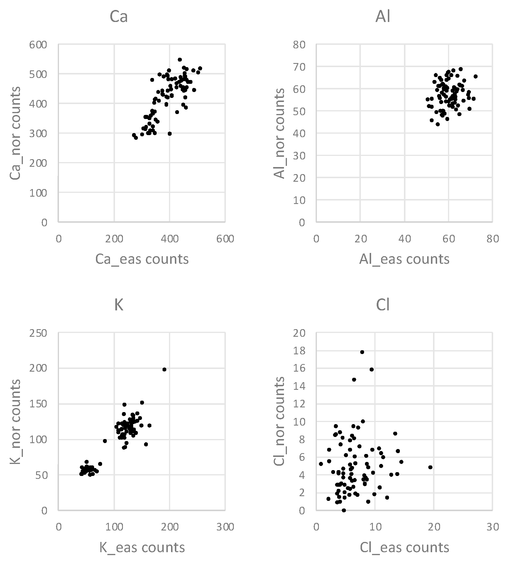
Table S2 in the Supplementary Material shows that smaller or larger but the mean elemental counts in the tree rings definitely vary. Aluminum shows a relatively small variation while chlorine shows a large one.
Figure 5 gives an example of two-dimensional distributions of the series of counts taken in the eastern direction of the stem vs. the series in the northern direction. The example shows that the absence of correlation in Al and Cl is due to discordant variation of the variables. On the contrary, the Ca and K counts from the eastern and northern radii variate mostly concordantly (
Figure 5).
Further exploration of the high correlations shown by Ca and K (
Table 1 and
Table 2) reveals that the possible source of the correlations is the macrotrend in the count values across all the tree rings. In other words, the count values in the inner tree rings are steadily different from those in the outer tree rings.
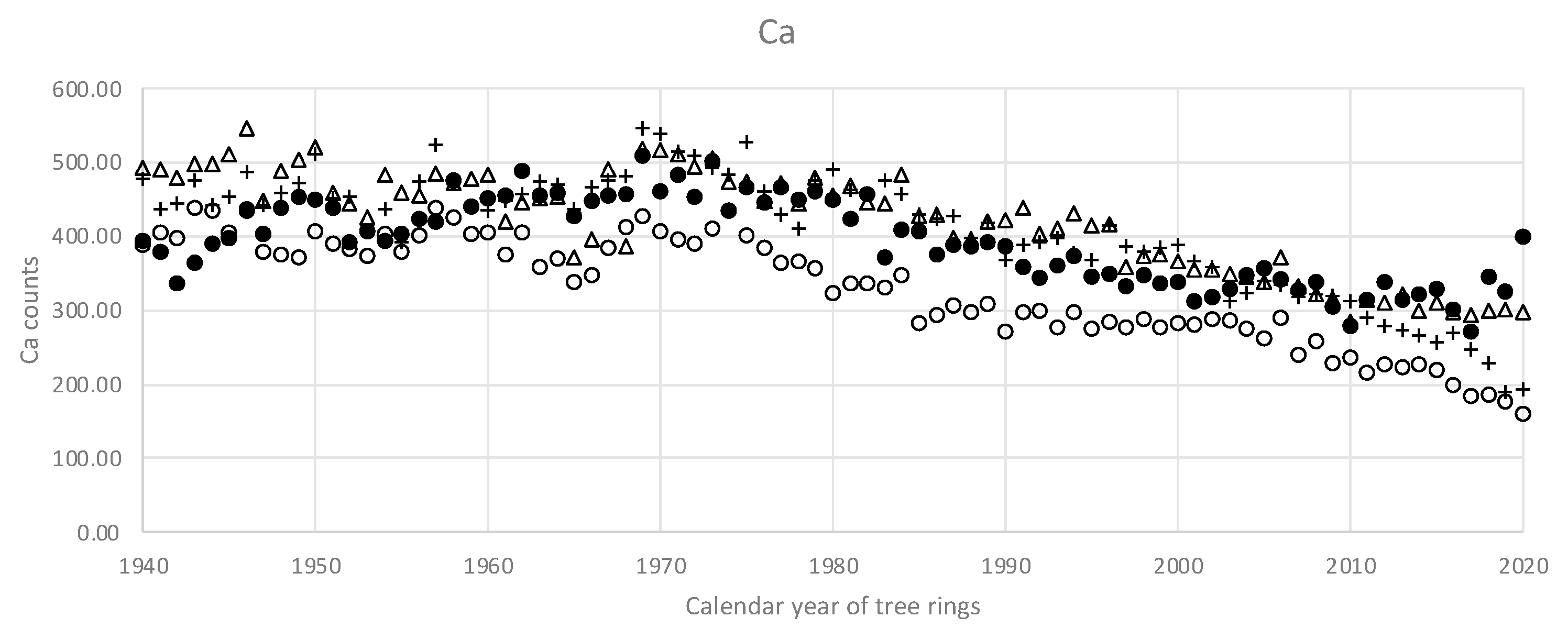
Figure 6 and
Figure 7 give an idea of the Ca and K macrotrends in the stem of pine #1.
In a sense, the macrotrends (
Figure 6 and
Figure 7) present a sort of low-frequency dynamics that comprises the whole range of observed years, i.e., many decades. This low-frequency structure is highly likely to produce the observed low-frequency correlations. On the other hand, it is the high-frequency correlations—that reflect the year-to-year variations—that are of special interest for dendrochemistry.
The resultant correlations after the detrending procedures (see Materials and Methods) are given in
Tables S3 and S4. In the tables, the correlation coefficients with no detrending are given for comparison. The significant correlation coefficients for the detrended data are marked by a yellow background and a bold (for
p < 0.001) or normal (for
p < 0.05) font.
Overall, in some cases, the detrended data show significant correlations. In some trees (e.g.,
Table S3, pine #1), the detrended data from the same cardinal directions give significant correlations (see the coefficients for Hugershof function, smoothing spline function, and derivatives detrending), which might be the reflection of a high-frequency correlation. However, a consistent inter-tree pattern can hardly be extracted from the data. Among all the significant correlations for, e.g., spline detrended Ca data (13 cases) nine are related to the south direction. But, in some trees, no single significant correlation is seen (pine #2). So, all the trees vary rather individually in the high-frequency dimension.
4. Discussion
The opportunity to extract wooden cores from trees and analyze them is a powerful research method. The sampling of full cross-sections is a rather labor intensive and destructive, while the cores’ technique allows the researchers to obtain a massive amount of data embracing many sample trees and many species. The latter is very important—taking into account that intra- or inter-species variability may often be poorly known beforehand.
Dendrochronology has used the opportunity of the cores’ technique to the full [
1]. In the neighboring research areas, however, which also use tree rings as a data carrier, some methodological questions may be still unanswered. For example, Pearson et al. [
23] found little agreement among five studied trees of
Pinus longaeva D.K. Bailey regarding the patterns of elemental distribution across the tree rings. Vives et al. [
24] reported a heterogenous distribution of a number of elements in
Pinus sp. wood samples, which, according to the authors, indicated the irregular ability of wood to preserve elements across the tree rings. Ferretti et al. [
25] reviewed important issues related to the use of dendrochemistry in aerial pollution studies. They overviewed possible uncertainties in the field and urged us to pay special attention to the sampling procedures to avoid a bias in the interpretations that follow the measurements. In our view, it would be pertinent to develop a common standard as to how to sample cores for a dendrochemical analysis.
The width of tree rings cannot change after the growth has been completed but elements may migrate in the wood. Due to the obvious technical complexity, studies on the elemental migration in wood are scarce and often limited to a single species. It has been reported, however, that some elements (Ca, Na, and K) translocated while other elements (Ti, Mn, Fe, Cu, Zn, P, and others) did not in the wood of pitch pine (
Pinus rigida Mill.) [
20]. Speer [
20] has reviewed some of the studies. They are rather various, both regarding the species involved and the elements considered. To our best knowledge, in vivo migration of elements in the wood of
P. sylvestris has not been yet reported. However, it’s natural to anticipate that such a migration may exist. For example, Bindler et al. [
26] reported that Pb isotopes in
P. sylvestris tree rings do not match the occurrence of lead pollution from other sources (peat), which may mean that lead might translocate from the place of uptake.
The probable elemental variability across tree rings puts an obvious question of how reliable a core extracted from one side of a tree stem is—in the respect of its representativeness of the elemental distribution pattern in that stem. The representativeness may be of a number of scales, but, for clarity, one can speak of a high-frequency agreement of the elemental contents around the circle and a low-frequency agreement. The high-frequency refers here to year-to-year variations (e.g., in
Figure 4a) while the low-frequency refers to long trends covering the whole lifetime of a tree (e.g.,
Figure 4d).
An important part of the present study is the search for consistent relationships. As follows from
Table S1 (Supplementary Material), practically no elements show (i) large enough and (ii) consistent intra-elemental correlations. This means that one can see a strong correlation between a pair of cardinal directions in a tree while the correlation is not repeated in another tree. In a sense, such a picture may be a result of inconsistent elemental distribution around the circle in the tree rings, as shown in
Figure 4b. Thus, it is hard to anticipate that the majority of the elements’ sequences from a pair of cores from different cardinal directions can show a high-frequency correlation. Obviously, it is evidence of the complexity of the processes that take place in a tree at the time of growth and right after the tree-ring growth has been completed.
The exceptions from the pattern present Ca and K. Their intra-elemental correlations are consistently strong among the sample trees. However, the source of the correlations was found to be the long-term trends. Mean calcium counts mostly drop down from the pith to the bark, while mean K counts grow from the pith to the bark. It is noteworthy to mention that the long-term trends take place rather concordantly within one tree stem. In the context of the study, it means that one core would most probably reliably represent the whole stem—if it goes about a low-frequency Ca or K variations. It is important to mention that the long-term Ca and K trends are widely found among trees of various geographical areas. For example, the
Avicennia species, a mangrove tree, shows the same stem-scale trend for Ca and K [
27] as has been observed in the current study.
The latter result is a promising one because of the role that Ca and K play in tree physiology. Among other metals, Ca shows the highest concentration in stem wood [
28], it is involved in the regulation of many of the tree’s physiological functions and is a significant structural component of cell stability [
29]. Chemically, calcium’s target is the carboxyl groups of pectin. Pectin provides rigidity to the cells being a structural component in the middle lamella and cell walls. The bounding of Ca into the cell wall prevents it from further participation in other processes [
29]. Besides the structural support, Ca plays a central role in cell signaling events and thus in cellular activity and responses [
30,
31].
As has been said, the high-frequency elemental variations are of special interest in dendrochemical studies because they allow one to relate the environmental chemistry and climate records to the wood chemistry at the annual resolution. To clean the series of data from the long-term component, a usual way is detrending which may be performed through various methods.
The greatest problem with detrending is, however, that real detrending is possible when a theory exists that predicts the mathematical form of the trend—so, that the trend, and the trend only, may be subtracted from the data series. To our best knowledge, no such a theory is nowadays available that can help with the description of the trends that govern the distribution of elements across tree-rings in trees. To a large extent, one has to match the detrending functions ‘by the sense of touch’ basing it rather on common sense.
The Hugershof curve has been designed to describe biological growth, and, from experience, it is most successful in detrending tree-ring widths. However, whether the distribution of the mean elemental content should follow the growth of a tree stem is an open question. The Hugershof curve does follow the elemental trends quite successfully but it obviously cannot fit in the trends in some trees. That is, the curve cannot sometimes help to remove the trend, which results in that it produces another trend, and some strong low-frequency correlations persist (see
Table S3, pine #3, and
Table S4, pines #1, 2, 3, 6). Obviously, the Hugershof curve may be too rigid for some data, especially for K trend data.
On the other hand, the spline approach presents quite a flexible instrument to detrend the series of data. The spline itself is not a single function but a combination of polynomes. Because of this spline feature and the spline’s high flexibility, there may be a suspicion that the spline-based detrending may remove not only a low-frequency trend but also the high-frequency variability. Nevertheless, after the spline-based detrending, there are enough significant, though weak, correlations, especially in Ca data (
Table S3).
The derivative approach is not bound to a model or detrending function. Its use as a detrending approach is based on the anticipation that—if the high-frequency correlation does exist—the increments would show a concordant behavior irrespective of how large or small the absolute value may be. That is, it’s a situation when the mean elemental counts synchronously go up in a pair of successive years and drop down in others. After the derivative-based detrending, there are quite numerous significant correlations. In a selected case, the correlation matrix may be filled by significant coefficients (
Table S4, pine #3).
To summarize the detrending analysis, the general picture is that there are sparkles of significant high-frequency correlations but there is an obvious lack of consistency among the studied trees. Irrespective of which of the three detrending approaches have been applied the resultant high-frequency correlations vary unpredictably from tree to tree.
5. Conclusions
To conclude, it may look like the results of the research are rather negative. In fact, at least for Scots pine, it is hard to anticipate that a random core may provide a repeatable year-to-year variation of the elemental content across the tree rings. It means that a reliable reconstructive analysis of the environmental chemistry is unlikely if one base is a unique core. The only opportunity for a reliable analysis with one core is the study of long-term trends shown by Ca and K—in the case of interest to the elements.
Still, some positive perspective is possible. First, one could use several cores taken from one tree, though, with the obvious increase in labor intensity.
Second, through immolation of the year-to-year resolution, one could hope to see stronger correlations with the use of wider time intervals that average data for three-, five-year or longer intervals. As the experience shows [
32], such data aggregation improves the correlations of elemental content with weather records. A probable cause for this is the averaging of the elemental migration in wood but this question is not well studied.
Third, it is quite probable that the chemical treatment of cores may improve the visibility of elements as has been shown in [
32].
Lastly, among various tree species, there may be species that perform better than others in the binding of elements in the xylem. So, a search for suitable tree species may well be a good research area.
The strategic direction in the field is, however, the discovery of inner wood chemistry that specifies how the elements are absorbed and released by the wood grain.

 ,
, 


