Article

Can Gap-Cutting Help to Preserve Forest Spider Communities?

1
Centre for Agricultural Research, Plant Protection Institute, ELKH, 1022 Budapest, Hungary
2
ELKH-ELTE-MTM Integrative Ecology Research Group, Eötvös Loránd University, 1117 Budapest, Hungary
3
Centre for Ecological Research, Institute of Ecology and Botany, 2163 Vácrátót, Hungary
4
Department of Plant Systematics, Ecology and Theoretical Biology, Eötvös Loránd University, 1117 Budapest, Hungary
5
Forestry Faculty, Institute of Environmental Protection and Nature Conservation, University of Sopron, 9400 Sopron, Hungary
*
Author to whom correspondence should be addressed.
Diversity 2023, 15(2), 240; https://doi.org/10.3390/d15020240
Submission received: 7 January 2023 / Revised: 3 February 2023 / Accepted: 7 February 2023 / Published: 8 February 2023
(This article belongs to the Special Issue Forest Spider Communities Diversity)

Abstract

:
Continuous cover forestry maintains many characteristics of uneven-aged natural forests and aims to preserve biodiversity. Gap-cutting is a management option that may create a balance between timber production and continuous forest cover. We investigated the effect of newly created gaps on ground-dwelling spider assemblages in a managed oak forest, in the Pilis Mts., Hungary. Between 2018–2021 we sampled newly created elongated and circular-shaped gaps of two different sizes in a six-times replicated randomised complete block design. Pitfall samples of ~4600 spiders indicated that spider species richness was moderately higher in the gaps than in control stands. Spider assemblages did not respond in a specific way to the different gap implementations, but their variation in species composition was considerably higher in gaps than in the control plots. The excess spider abundance and species number in gaps, as compared to control, increased over the observation period, as did the dissimilarity of gap assemblages to control. Species responses imply that gaps create a variation in microhabitats and microclimatic conditions, resulting in spiders’ diversification. The overall effect of gaps on spider assemblages suggests that gap-cutting is a suitable management option that preserves forest spider assemblages.

1. Introduction

One of the many conflicts between mankind and the natural environment is the constant human demand for natural resources such as timber or firewood from forests. It is therefore important to strike a good balance between the rational use of natural resources and the conservation of biodiversity in semi-natural forests. This issue is also true for forest management, where the sustainable use of forests and woodlands for timber production is crucial for future generations [1]. In addition, semi-natural forests provide a wide range of ecosystem services, including the maintenance of a healthy environment, soil formation, oxygen production and carbon sequestration [2,3]. Forests also provide important cultural services in the form of tourism, recreation and inspiration [4].
Continuous cover forestry (CCF) is a management system that, by avoiding large cutting areas, continuously maintains the physiognomical characteristics of an uneven-aged natural forest [5], and therefore promises to perform better than rotation (periodically clear-cut) systems in keeping up ecosystem services, as well as in preserving biodiversity [6]. It shows higher similarity to the natural disturbance regime of the temperate forests than rotation systems [7]. The continuity of the uneven-aged forest cover is a primary feature of CCF, although judging continuity is obviously scale-dependent [8]. An important consideration of management is the feasible extent of selective removal of trees, including the creation of gaps of different sizes [9]. At larger scales, CCF should aim to bring about horizontal and vertical variability in forest structure, allowing for the promotion of tree species diversification and a wide age structure of trees. Such management practices may lead to economically viable alternatives to managing initially dense even-aged stands in rotation systems, because natural processes, such as regeneration and self-thinning may naturally lead to a desirable forest structure that produces quality timber; furthermore, CCF may sustain a constant amount of timber over time [10].
One way of implementing CCF is the creation of canopy gaps by harvesting small groups of trees or single tree individuals. These gaps modify light and other microclimatic conditions and are the main areas for tree regeneration [11]. The formation of artificial gaps in the long term creates horizontal and vertical variation, which is one important aim of CCF. Gap-cutting mimics natural forest dynamics since these openings should have a similar effect as tree-fall gaps in unmanaged forests, which leads to a diverse collection of regenerating tree species [12]. Gap sizes also depend on management goals, e.g., the light and moisture requirements of tree species preferred by production. In mixed oak forests both in North America and in Central Europe, gap sizes typically range from 100 to 5000 m2 [9,13,14]. Gaps considerably alter microclimatic conditions locally. Compared to other management methods, canopy gaps created by gap-cutting provided a more illuminated environment, although with an irradiance significantly lower than that of clear-cut areas [15]. Overall, gaps can maintain a buffered environment providing more available light and consumable soil moisture and temperatures less raised than in clear-cuts [15]. However, at a stand scale, the relatively low proportion of these openings does not change the continuous nature of forest cover and climatic conditions [16]. Gap-cutting significantly affects the cover, height and species composition of understory vegetation [17] as well as several invertebrate taxa on the forest floor [18] including spiders [19]. However, whichever component of the forest biota is considered, the effect of gaps may largely depend on particular gap size, shape, exposure and orientation [11].
To convert a significant proportion of forests to the continuous cover forestry system, it is crucial to select a pre-tested optimal size and shape for gap openings. Gap shape, size and orientation usually serve forestry goals. However, other desirable outcomes, such as the maximal preservation of forest biodiversity, might also be achieved by careful optimization of gap parameters. Different gap designs cause different effects on multiple conditions of the forest ecosystem such as light, soil moisture, temperature, and nutrients, which consequently affect the understory vegetation and forest regeneration [11]. Within this framework, we would like to know how different implementations of gap-cutting affect forest spider communities in a Hungarian oak-hornbeam forest stand. We aimed to study the effect of newly created gaps of different shapes and sizes. In a randomized block experiment, we intended to explore how local ground-dwelling spider communities changed in these gaps as compared to unmanaged control plots.

2. Materials and Methods
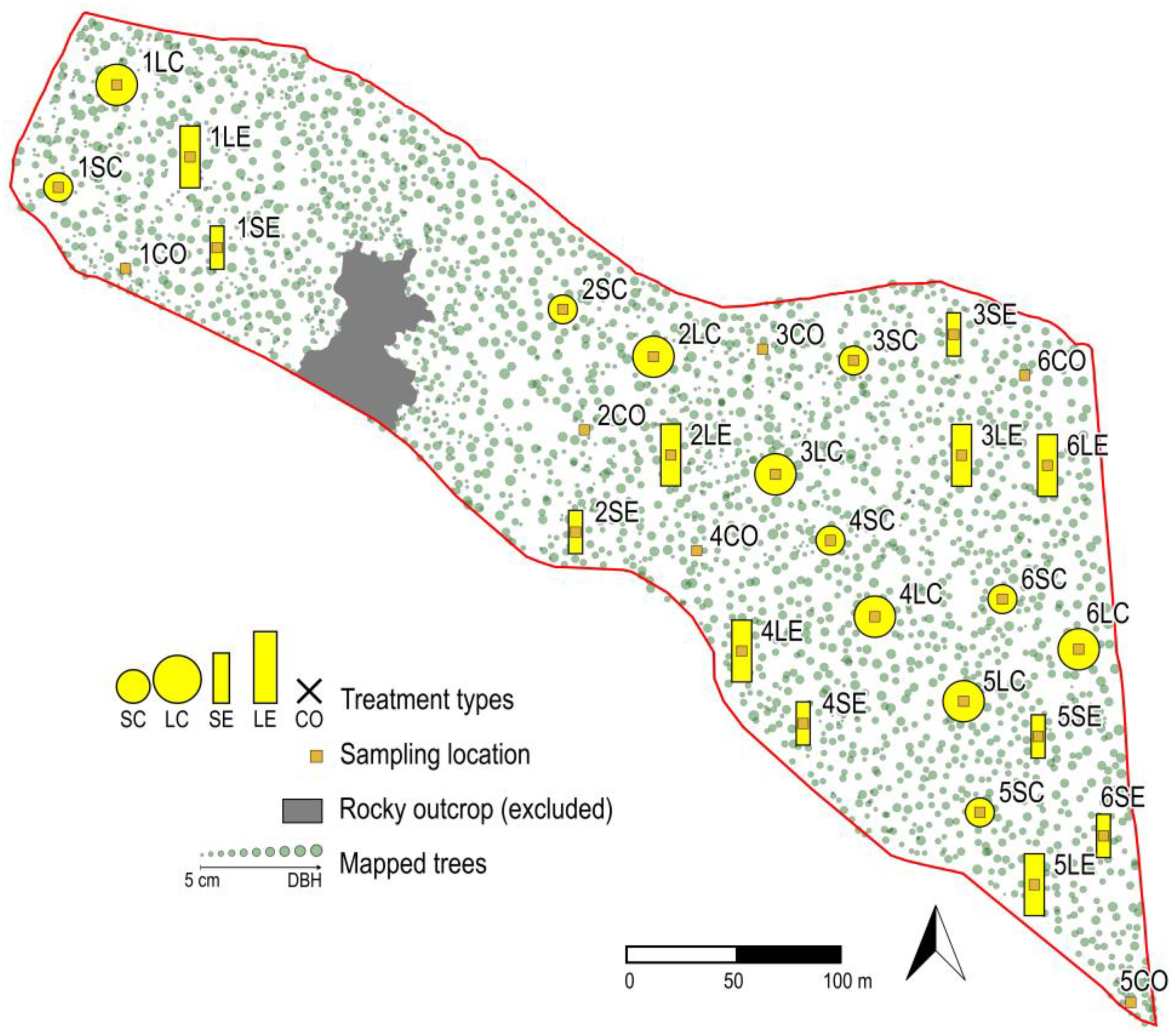
2.1. Study Area

The Pilis Gap Experiment (https://piliskiserlet.ecolres.hu/en) was located in a 10 ha sized 90-year old oak–hornbeam forest stand (centre point: 47°40′ N, 18°54′ E) in the Pilis Mountains in the vicinity of Pilisszántó, Hungary. The stand is surrounded by mature forests and is located in a continuously forested landscape. The elevation of the area is 390–460 m a.s.l., the average annual mean temperature is 9.0–9.5 °C, with a mean annual precipitation of 600–650 mm [20]. The bedrock consists of limestone and red sandstone with loess. The dominant soil type of the area is luvisol and rendzic leptosol, soil depth varied between 70 and 150 cm [15]. The stand is an ancient (long-continuity) forest, but it has been regularly managed, recently by the shelterwood silvicultural system, resulting in an even-aged, structurally homogenous stand. The canopy layer was dominated by sessile oak (Quercus petraea (Matt.) Liebl.), with a mean tree height of 23 m and a mean diameter at breast height (DBH) of 38 cm. The canopy layer also contained turkey oak (Quercus cerris L.) as subdominant species. Hornbeam (Carpinus betulus L.) formed a secondary canopy layer at 14 m height (mean DBH of 17 cm), where manna ash (Fraxinus ornus L.) appeared as a subordinate species. The shrub layer was scarce, and the cover of the herbaceous understory layer was closed (almost 100%), dominated by Carex pilosa Scop. and Melica uniflora L.

2.2. Sampling Design and Data Collection

We established five gap formations (treatments) using a randomised complete block design [21] with six blocks as replicates (Figure 1). The various gap scenarios in terms of shape and size complied with local forestry routine and were based on the management-oriented interest of forestry enterprises in Hungary:
  • Control (CO): mature, closed-canopy stand without any treatment;
  • Large Circular (LC): a circular gap with a 10-m radius (i.e., total length of one mature tree) and the approximate size of 300 m2. This type may represent the most common approach for gap-cutting in the study area, although the managers achieve this size in several steps in time, and the shape might be slightly irregular due to spatial constraints;
  • Small Circular (SC): a gap with a 7-m radius that corresponds to 2/3 of the length of a mature tree, with an area of 150 m2;
  • Large Elongated (LE): a large gap of elongated type, also with N-S orientation (width: 10 m, length: 30 m) and in the same size as LC;
  • Small Elongated (SE): a gap where trees were removed along a longitudinal axis (width: 7 m, length: 21 m) with N-S orientation to avoid the large extent of direct radiation and in the same size as SC.
Figure 1. Design of the gap experiment in the experimental forest stand in the Pilis Mountains. Green dots indicate trees, with dot size relative to the diameter of the trunk at breast height (DBH). Yellow circles and rectangles show the positions and types of gaps created. We investigated two gap sizes (150 and 300 m2) and two gap shapes (circular and elongated). Notation of the gap treatments is the following: SC = small circular, LC = large circular, SE = small elongated, LE = large elongated. Small rectangles indicate sampling locations in the centre of the gaps, where pitfall traps were placed in a triangular formation. Rectangles outside gaps show the sampling locations for control plots (CO). Numbering of plot nametags refers to which block they belong to.
Diversity 15 00240 g001
The treatments were implemented during the winter of 2018/2019. The resulting 30 plots (5 treatments × 6 replicate blocks) were considered the basic sampling units. Blocks were defined by the spatial proximity of the plots and were not separated by physical barriers or by any sort of discontinuity in the forest stand (Figure 1).
Data collection followed the concept of Before-After Control-Impact (BACI) experiments [15,19], i.e., first surveying the spider assemblages from the growing season of 2018 (before the implementation) and then through 2019–2021 (post-implementation years) with the same protocol. Sampling locations were established in the centre of every plot (Figure 1), where three pitfall traps were installed in the corners of a triangle of 2 m sides to sample ground-dwelling invertebrates, such as spiders. In total, we surveyed 90 pitfalls. Each year, the community was sampled in late-spring (June) and autumn (September) for one month corresponding to the highest activity regime of spiders and other ground-dwelling arthropods (e.g., carabids), which was based on personal observations and the literature data [22,23]. The traps were made of 85 mm diameter plastic cups; each containing approximately 250 cm3 of a 50% solution of propylene glycol and water, saturated with salt and with a drop of odourless detergent to reduce surface tension. A dark green plastic roof protected the solution from litter and rain. For spider identification, we used an internet-based key [24]; taxonomy followed the World Spider Catalog [25]. Activity density data of pitfall traps from the same plot and same year were merged, and thus the elementary sampling units of the analyses were yearly catches in the plots. The term activity density refers to the empirical fact that catches of pitfall traps depend on the individuals’ activity; the higher activity of the individuals, the more catches in the traps [26]. Although activity density might be the most accurate proxy for pitfall catch data, the most commonly used term is abundance, thus we use this term hereafter.

2.3. Statistical Analysis

In order to test the effectiveness of the applied sampling effort, we estimated the mean expected species richness in the studied forest site with the Mao Tau estimator using a sample-based rarefaction method [27] in the ‘vegan’ package [28] for R 4.2.2 [29]. The confidence intervals were generated from 10,000 reshufflings of the sample order. In addition, we portrayed the rank-abundance plot for the whole spider assemblage to explore how the dominant species contribute to the total number of catches [30].
For the univariate analyses, we used the software JMP [31]. Ordination methods were applied using Canoco 5 [32,33]. Overall treatment effect on (square root transformed) spider abundance and species richness for the post-implementation years was analysed with Linear Mixed-effect Models (LMM), where we included block and study year as nested random effects to account for spatial and temporal blocking effects. Cohen’s d effect sizes between control and gap treatment types were calculated on untransformed data [34]. To assess whether species abundance and richness in treatment plots were diverging from the control over time, in the LMMs, we modelled the effect of the year as a continuous variable, treatment as a fixed variable and block as a random variable on the difference in richness and abundance between control and treatment plots. Post hoc differences in treatment effects were tested with the Tukey HSD test.
The response of spider species composition to gap treatments in the post-implementation years was examined by unconstrained ordination analysis [32]. As the Detrended Correspondence Analysis showed a 2.6 SD unit long gradient in the species composition response data, we continued with a linear unconstrained ordination analysis as suggested by [32], in particular with Principal Components Analysis (PCA). To depict community composition changes over time relative to control for the whole study period, we performed a Principal Response Curves (PRC) analysis [35]. PRC calculates scores for a single ordination axis based on the scores of an RDA, in which time (years in our case) was the covariate and the single explanatory variable was the interaction between treatment and time. The significance of the explanatory variable was tested with Monte Carlo permutation test.

3. Results

Over the four years of the study, we have collected 4579 spider individuals, out of which 3770 were adults and identified to species level, representing 31 species from 18 families (Appendix A Table A1). The remaining 933 juveniles of various stages were only identified at higher taxonomic levels. Juveniles represented nine genera that were not represented in the species-level identification, including Philodromus sp. and Anyphena sp., which also added to the family count. Considering this, the minimum number of species recovered during the study was 40 in 20 families. However, given that most individuals that were identified to genus level could represent more than one species, juvenile data were altogether excluded from analyses that required species-level distinction.
The rarefaction curve computed for the entire adult data set (Figure 2a) revealed that the sampling effort not fully, but satisfactorily represented the ground-dwelling spider assemblage that could be sampled in the applied sampling periods. Over 80% of the total number of species sampled (25 of the 31 species) was collected considering only 50 sampling units, which is less than half of the total number of sampling units (N = 119). The rank-abundance plot showed (Figure 2b) that four species (Urocoras longispina, Psammitis sabulosus, Pardosa lugubris and Trochosa terricola) were dominant, each representing greater than ten percent of the total adult catch.
Considering the post-implementation years, spider abundance in the various gap treatment plots and in control plots did not differ from each other (LMM, treatment effect: F = 1.62; d.f. = 4, 78; P = 0.178; Figure 3a). The random effect of the year explained 29.8% of the total variance, whereas block effect accounted for 10.9% of the total variance. Treatment effect on species richness was significant (LMM, treatment effect: F = 3.51; d.f. = 4, 78; P = 0.01; Figure 3b). Species richness was not statistically different among the gap types, and the same phenomenon was observable regarding Shannon diversity (Appendix A Table A1). Concerning species richness difference from the control, although nominally all treatments resulted in higher richness than in control as the Tukey HSD test indicated (Figure 3b), specific significant differences occurred only between the two elongated gap types and controls. The calculated Cohen’s d effect sizes underlined that these are in fact considerable richness differences. Largest difference was observable between LE and control sampling units (dCO-LE = 1.08), and the mean effect size between control and the gap treatments was also substantial (mean dCO-gaps = 0.82). The random effect of year was considerable, explaining 39.6% of the total variance, whereas the block effect was considerably smaller, accounting for 3.6% of the total variance.
To follow up on how abundance and species richness changed over the study years relative to the control, we calculated a control-treatment abundance and richness difference for each plot and year. The LMM models showed that there was no significant treatment effect, i.e., the control-treatment difference was not dependent on the type of gap treatment, neither in terms of abundance nor species richness. However, in the case of both measures, the control-treatment differences gradually increased over time during the observation period (effect of year, abundance difference: F = 4.99; d.f. = 1, 86; P = 0.0281; Figure 3c; effect of year, species richness difference: F = 13.58; d.f. = 1, 86; P = 0.0004; Figure 3d). The random effect of the block was small (5.53% of total variance) in the case of abundance difference, whereas it was larger (28.8% of total variance) in the case of richness difference.
Species composition changes in the various treatment plots were investigated with PCA. The first and second axes of the ordination cumulatively explained 35.8% and 52.6% of the total variance, respectively. Considering only the post-implementation years (i.e., 2019–2021), the ordination plot (Figure 4a) revealed that species assemblages in the control plots of the different blocks were relatively close together. In contrast, species assemblage compositions in the gap treatments overlapped with control assemblages but showed a greater variation. They occupied a larger ordination space than the controls but were very similar to each other (Figure 4a).
The Principal Response Curves showed, on one ordination axis, that assemblages were very similar in year zero when all treatments were “control”, as the gap treatments had not been implemented yet. After implementation (i.e., executing gap-cutting), the divergence from control assemblages variably increased over time and reached its maxima in the second and third years. The PRC of the circular and elongated gaps were different regardless of their diameter, elongated gaps had a stronger treatment effect with maxima in the third year, while circular gaps had a weaker effect, but it showed earlier maxima in the second year (Figure 4b). Overall treatment effect on the spider assemblages, as compared to control was significant as indicated by a Monte Carlo permutation test (F = 0.4; P = 0.046; Figure 4b).

4. Discussion

Gap treatments change the forest canopy cover, and consequently microclimatic conditions, foremost light availability, air and soil temperature, and soil moisture at relatively small scales [11]. The present study revealed that gap creation, as means of a continuous cover forestry management system, causes relatively small changes in forest spider assemblages. Spider diversity, described by species numbers, was moderately higher in the newly created gaps, and species compositions showed greater variability compared with untreated plots in the forest. These are important insights into forest ground-dwelling arthropod dynamics because, as previous studies in the same forest stand revealed, other, more drastic silvicultural treatments had a considerable impact on a range of invertebrate taxa, including spiders [18,19]. Different taxa showed contrasting responses to a wider range of forestry treatments, which both depended on the specific tolerances of the taxa to environmental variables and their dispersal ability. For instance, enchytraeid worms with limited dispersal ability and sensitivity to soil moisture reacted the strongest to the environmental changes caused by the treatments, dramatically decreasing in the retention tree treatment where evapotranspiration decreased soil moisture [36]. In contrast, the increased light levels resulted in an intensive growth of the understory vegetation in the clear-cut plots [17], which was favourable for spiders, which increased their species richness by the immigration of open habitat species [19], but not for carabids, which responded less promptly by dispersal and lost some of the forest specialist species in the clear-cut plots [18].
Spiders are effective indicators of the environmental and biotic states of a habitat [37,38]. Spiders are sensitive to different disturbances in a forest. They respond promptly to changes in the abiotic environment that are often associated with forestry treatments [39], including altered light regimes and moisture levels [19]. The spider community reacts both to the extent and severity of disturbances. Small and medium disturbances—in line with the intermediate disturbance hypothesis [40] (but also see [41,42])—often result in an increase in spider diversity [19,43], but severe disturbances have a clear negative impact on spiders [44]. Disturbances create structural changes in the habitat, which crucially affects spiders because vegetation gives structural support to the webs of web-building species. Such changes indirectly influence microclimate and prey availability, which affects non-web builders, too [45,46]. Due to their ballooning behaviour, spiders are good dispersers and can promptly occupy newly created or modified habitat patches, indicating environmental changes rather rapidly. Spiders were the quickest group to return to a regenerating juniper habitat after fire [47] and also responded more promptly to silvicultural treatments than groups with more limited dispersal capability [18]. Given the prompt and effective indicator potential of spiders, any robust sign of lack of indication should also be considered informative.
The indication potential of spiders for the comparison of different habitat types or habitats that were affected by different environmental impacts, such as forestry treatments, can be realised if the applied sampling method(s) represent differences in the assemblages adequately. Pitfall trapping is a well-established sampling method to describe arthropod assemblages, including spiders [48], but its specificity and limitations have to be taken into account. These include that pitfall trapping is a stratum-specific method, which samples ground-dwelling arthropods [48]. Pitfall trap catches cannot be directly translated to density figures [49], catches depend on body size, sex, season and even species-specific activity [26,50]. Still, since most of the factors listed above act similarly in the compared habitats, pitfall trapping is a proven method for comparative purposes, e.g., [51,52], and, in specific, it has been successfully used to describe spiders in similar forestry experiments [53,54]. It was also shown that microhabitat variations, such as those caused by forestry treatments, do not significantly influence pitfall capture efficiencies [55]. The degree of satiation of the rarefaction curve in the present experiment indicated that sampling adequately described the subset of the spider assemblage that was accessible by pitfalls.
Artificial gaps are favourable management options because gap creation causes relatively small-scale disturbances in the forest ecosystem and mimics the effect of natural tree falls and subsequent regeneration—the process termed gap phase dynamics [11,56]. The process contributes to the maintenance of tree diversity, as well as to the creation of structural and microclimatic heterogeneity [7,12]. Tree diversity was the main explanatory variable of spider species richness [54] and had a strong positive relationship with many other organism groups [57]. Gaps create a relatively fine-grained structural heterogeneity on a landscape scale, while traditional management regimes, such as clear-cutting and shelterwood systems result in large-scale homogenization, which, consistently across various taxonomic groups, leads to a local decrease in alpha diversity [58]. Gaps open up the canopy, but the increase in light is less than in the case of large-scale deforestation because of the shading effect of trees at the perimeter of the gap. Interestingly, the association of canopy openness with spider species richness was hump-shaped and showed a maximum at intermediate levels [59]. In the gaps, the locally missing evapotranspiration of trees results in higher moisture levels at the ground layer and a cooler microclimate than in the closed forest parts. A combination of high humidity and light intensity [16] leads to more dense forest floor vegetation [17] providing rich structure and favourable microclimate for both web-building and hunting spider species [60]. The response of other invertebrate groups to gap-cutting was moderate, laid between response to clear-cutting and control plots in an adjacent forest stand [18]. The border of a gap with the unmanaged forest stand creates an ecotone. Edge effects at the border of open and forested habitats include spillover shaping local communities [61]. Ecotones often accommodate edge specialist species which contribute to the gap fauna, as was found in gaps created in a Hungarian oak forest [62]. Thus, in our study, a moderate increase in spider species richness seems to be in line with the findings of other similar studies.
The spider assemblages in the various gap types have apparently responded to this type of forestry treatment, but these responses considerably overlapped among the different gap implementations. While spider assemblages in the control plots occupied a relatively compact ordination space, assemblages in the gaps expanded over a wider area and overlapped with each other; moreover, completely overlapped with the area of the control plots. Thus, the gaps likely increased environmental variability but without causing a disjunct separation from control. This expansion of assemblage compositions also had a temporal trajectory. While all plots were similar to each other in the pre-treatment year, starting with the first year after gap creation spider assemblages gradually but variably deviated from control assemblages. The few marginally significant differences suggest that maybe elongated gaps have a somewhat greater effect, and these effects also unfold slightly differently over time compared to how spider communities change in circular gaps. In the present study, we could follow the fate of the assemblages for four years. In a similar experiment, where a greater diversity of silvicultural treatments was applied, we found that spider assemblages started to approximate the control already in the fifth year [19].
Departure from the control state had no particular treatment-specific direction considering species compositions. Species-specific responses indicated that this diffuse departure is a composite result of rather dissimilar species responses. This suggests that the created gaps may differ from control plots in multiple ways. Most of the species that became more frequent in gaps could be characterised as associated with more open habitats. For instance, cursorial spiders, such as Pardosa lugubris (Lycosidae) and Drassyllus villicus (Drassidae) in other European locations were associated with more open oak-dominated forest habitats [63] and also occurred more frequently in silvicultural treatments that result in a higher degree of canopy openness [19]. Perpendicular to the response of moderately open forest species, the crab spider Psammitis sabulosus (Thomisidae) represented the most open end of the closed-open, drier-more humid habitat range. Histopona torpida (Agelenidae), displaying a completely reverse direction in the ordination space, indicated more closed woodland habitats [24]. Other species that did not show a strong response, such as Atypus affinis (Atypidae) and Zora spinimana (Miturgidae), are known to be mostly associated with leaf litter [64], a common microhabitat in all studied habitat patches. Metacommunity processes [65], such as the aforementioned spillover and immigration-emigration from the forest matrix, are likely to be further factors in not seeing more marked species responses.
The Pilis Gap Experiment sought to find out the extent to which gap-cutting and its various implementations, as a management option of CCF, affects different elements of the forest ecosystem. Spiders are robust indicators of environmental changes, including possible detrimental effects of different silvicultural practices. The present study gave evidence that spider assemblages were not negatively influenced by any of the gap-cutting schemes; rather, species richness increased in the created gaps. The effect of different gap implementations could not be distinguished on the spider assemblages. Species responses imply that gaps create a variation in microhabitats and microclimatic conditions, which results in the diversification of spiders. This case study on spiders suggests that gap-cutting is indeed a viable and unharmful way to achieve CCF. It shows that, at least on the present scale, the effect of different gap implementations do not differ from each other, thus the response of other indicator groups and/or forestry objectives should decide the actual practices.

Author Contributions

Conceptualization, P.Ó., Z.E. and F.S.; methodology, P.Ó., B.K., Z.E. and F.S.; field sampling, Z.E. and J.R.; validation, P.Ó., Z.E. and J.R.; statistical analysis, F.S.; laboratory work, taxonomic identification: E.B.; data curation, F.S. and E.B.; writing—original draft preparation, F.S.; writing—review and editing, F.S., Z.E., P.Ó., E.B., J.R. and B.K.; visualization, F.S. and B.K. All authors have read and agreed to the published version of the manuscript.

Funding

The study was supported by the National Research, Development and Innovation Fund of Hungary (OTKA K128441, K143270) and the Hungarian Academy of Sciences (MTA Sustainable Development and Technology National Programme). BK was supported by the ÚNKP-22-4 New National Excellence Program of the Ministry for Culture and Innovation from the source of the National Research, Development, and Innovation Fund.

Institutional Review Board Statement

Not applicable, the study involved only arthropods, for which no ethical approval was needed.

Data Availability Statement

Aggregated basic data are presented in Appendix A. Raw data can be obtained from authors on reasonable request.

Acknowledgments

The authors are thankful Csaba Németh for the stand structural inventory of the forest. The implementation of the treatments is acknowledged to the colleagues of Pilis Park Forest Company, Péter Csépányi and Viktor Farkas.

Conflicts of Interest

The authors declare no conflict of interest.

Appendix A

Table A1. List of species by spider family and their total catches by treatments. Abbreviation of treatments: CO = control, LC = large circular, LE = large elongated, SC = small circular, SE = small elongated.
FamilySpecies NameTreatment
COLCLESCSE
AgelenidaeHistopona torpida (C. L. Koch, 1834)1613272514
AgelenidaeUrocoras longispina (Kulczynski, 1897)324166204280233
AraneidaeCercidia prominens (Westring, 1851) 1
AtypidaeAtypus affinis Eichwald, 1830911131014
ClubionidaeClubiona neglecta O. P.-Cambridge, 186226214030
ClubionidaeClubiona terrestris Westring, 1851 1
DysderidaeDysdera erythrina (Walckenaer, 1802)10619210
DysderidaeDysdera ninnii Canestrini, 186821113
DysderidaeHarpactea rubicunda (C. L. Koch, 1838)155 34
GnaphosidaeDrassyllus villicus (Thorell, 1875)438493033
GnaphosidaeHaplodrassus silvestris (Blackwall, 1833)812181212
GnaphosidaeTrachyzelotes pedestris (C. L. Koch, 1837)114302312
HahniidaeCicurina cicur (Fabricius, 1793) 1
LinyphiidaeDiplostyla concolor (Wider, 1834) 1
LinyphiidaeTapinopa longidens (Wider, 1834)1 1
LinyphiidaeTenuiphantes flavipes (Blackwall, 1854) 1
LiocranidaeAgroeca brunnea (Blackwall, 1833)91961813
LiocranidaeLiocranoeca striata (Kulczynski, 1882) 1
LiocranidaeScotina celans (Blackwall, 1841) 1344
LycosidaeAulonia albimana (Walckenaer, 1805) 1 1
LycosidaePardosa lugubris s.str. (Walckenaer, 1802)2720318373107
LycosidaeTrochosa terricola Thorell, 185610574114100110
MimetidaeEro furcata (Villers, 1789)11 1
MiturgidaeZora spinimana (Sundevall, 1833)1 573
PisauridaePisaura mirabilis (Clerck, 1757) 1 2
SalticidaeEvarcha arcuata (Clerck, 1757) 1 1
SalticidaeMarpissa nivoyi (Lucas, 1846) 1
SparassidaeMicrommata virescens (Clerck, 1757) 1
TetragnathidaePachygnatha degeeri Sundevall, 1830 1
ThomisidaePsammitis sabulosus (Hahn, 1832)115118192145137
ZodariidaeZodarion rubidum Simon, 1914 6353
Total number of adult individuals650700891780749
Number of species1723191923
Shannon diversity1.602.022.082.032.09

References

  1. Kraus, D.; Krumm, F. Integrative Approaches as an Opportunity for the Conservation of Forest Biodiversity; European Forest Institute: Freiburg, Germany, 2013. [Google Scholar]
  2. García-Nieto, A.P.; García-Llorente, M.; Iniesta-Arandia, I.; Martín-López, B. Mapping forest ecosystem services: From providing units to beneficiaries. Ecosyst. Serv. 2013, 4, 126–138. [Google Scholar] [CrossRef]
  3. Mori, A.S.; Lertzman, K.P.; Gustafsson, L.; Cadotte, M. Biodiversity and ecosystem services in forest ecosystems: A research agenda for applied forest ecology. J. Appl. Ecol. 2017, 54, 12–27. [Google Scholar] [CrossRef]
  4. Forest Europe. State of Europe’s Forests. In Proceedings of the Ministerial Conference on the Protection of Forests in Europe, Madrid, Spain, 20–21 October 2015. [Google Scholar]
  5. Pommerening, A.; Murphy, S.T. A review of the history, definitions and methods of continuous cover forestry with special attention to afforestation and restocking. Forestry 2004, 77, 27–44. [Google Scholar] [CrossRef]
  6. Peura, M.; Burgas, D.; Eyvindson, K.; Repo, A.; Mönkkönen, M. Continuous cover forestry is a cost-efficient tool to increase multifunctionality of boreal production forests in Fennoscandia. Biol. Conserv. 2018, 217, 104–112. [Google Scholar] [CrossRef]
  7. Aszalós, R.; Thom, D.; Aakala, T.; Angelstam, P.; Brūmelis, G.; Gálhidy, L.; Gratzer, G.; Hlásny, T.; Katzensteiner, K.; Kovács, B.; et al. Natural disturbance regimes as a guide for sustainable forest management in Europe. Ecol. Appl. 2022, 32, e2596. [Google Scholar] [CrossRef]
  8. Schall, P.; Gossner, M.M.; Heinrichs, S.; Fischer, M.; Boch, S.; Prati, D.; Jung, K.; Baumgartner, V.; Blaser, S.; Böhm, S.; et al. The impact of even-aged and uneven-aged forest management on regional biodiversity of multiple taxa in European beech forests. J. Appl. Ecol. 2018, 55, 267–278. [Google Scholar] [CrossRef]
  9. Mason, W.L.; Diaci, J.; Carvalho, J.; Valkonen, S. Continuous cover forestry in Europe: Usage and the knowledge gaps and challenges to wider adoption. Forestry 2021, 95, 1–12. [Google Scholar] [CrossRef]
  10. Kern, C.C.; Burton, J.I.; Raymond, P.; D’Amato, A.W.; Keeton, W.S.; Royo, A.A.; Walters, M.B.; Webster, C.R.; Willis, J.L. Challenges facing gap-based silviculture and possible solutions for mesic northern forests in North America. Forestry 2017, 90, 4–17. [Google Scholar] [CrossRef]
  11. Muscolo, A.; Bagnato, S.; Sidari, M.; Mercurio, R. A review of the roles of forest canopy gaps. J. For. Res. 2014, 25, 725–736. [Google Scholar] [CrossRef]
  12. Bauhus, J.; Puettmann, K.; Messier, C. Silviculture for old-growth attributes. For. Ecol. Manag. 2009, 258, 525–537. [Google Scholar] [CrossRef] [Green Version]
  13. Lhotka, J.M.; Cunningham, R.A.; Stringer, J.W. Effect of silvicultural gap size on 51 year species recruitment, growth and volume yields in Quercus dominated stands of the Northern Cumberland Plateau, USA. Forestry 2018, 91, 451–458. [Google Scholar] [CrossRef]
  14. Tobisch, T. Parent stand growth following gap and shelterwood cutting in a sessile oak-hornbeam forest. Acta Silvat. Lignar. Hung. 2010, 6, 33–48. [Google Scholar]
  15. Kovács, B.; Tinya, F.; Guba, E.; Németh, C.; Sass, V.; Bidló, A.; Ódor, P. The Short-Term Effects of Experimental Forestry Treatments on Site Conditions in an Oak–Hornbeam Forest. Forests 2018, 9, 406. [Google Scholar] [CrossRef]
  16. Kovács, B.; Tinya, F.; Németh, C.; Ódor, P. Unfolding the effects of different forestry treatments on microclimate in oak forests: Results of a 4-yr experiment. Ecol. Appl. 2020, 30, e02043. [Google Scholar] [CrossRef]
  17. Tinya, F.; Kovács, B.; Prättälä, A.; Farkas, P.; Aszalós, R.; Ódor, P. Initial understory response to experimental silvicultural treatments in a temperate oak-dominated forest. Eur. J. For. Res. 2018, 138, 65–77. [Google Scholar] [CrossRef]
  18. Elek, Z.; Kovács, B.; Aszalós, R.; Boros, G.; Samu, F.; Tinya, F.; Ódor, P. Taxon-specific responses to different forestry treatments in a temperate forest. Sci. Rep. 2018, 8, 16990. [Google Scholar] [CrossRef] [PubMed]
  19. Samu, F.; Elek, Z.; Kovács, B.; Fülöp, D.; Botos, E.; Schmera, D.; Aszalós, R.; Bidló, A.; Németh, C.; Sass, V.; et al. Resilience of spider communities affected by a range of silvicultural treatments in a temperate deciduous forest stand. Sci. Rep. 2021, 11, 20520. [Google Scholar] [CrossRef] [PubMed]
  20. Dövényi, Z. Magyarország Kistájainak katasztere [Cadastre of Hungarian Regions]; MTA Földrajztudományi Kutatóintézet: Budapest, Hungary, 2010. [Google Scholar]
  21. Scheiner, S.M.; Gurevitch, J. Design and Analysis of Ecological Experiments, 2nd ed.; Oxford University Press: New York, NY, USA, 2001; p. 415. [Google Scholar]
  22. Sapia, M.; Lövei, G.L.; Elek, Z. Effects of varying sampling effort on the observed diversity of carabid (Coleoptera: Carabidae) assemblages in the Danglobe Project, Denmark. Entomol. Fenn. 2006, 17, 345–350. [Google Scholar] [CrossRef]
  23. Jimenez-Valverde, A.; Lobo, J.M. Establishing reliable spider (Araneae, Araneidae and Thomisidae) assemblage sampling protocols: Estimation of species richness, seasonal coverage and contribution of juvenile data to species richness and composition. Acta Oecol. 2006, 30, 21–32. [Google Scholar] [CrossRef]
  24. Nentwig, W.; Blick, T.; Bosmans, R.; Gloor, D.; Hänggi, A.; Kropf, C. Spiders of Europe. Version 07. 2022. Available online: https://www.araneae.nmbe.ch (accessed on 6 January 2023).
  25. World Spider Catalog. World Spider Catalog; Version 23.5; Natural History Museum Bern: Bern, Switzerland, 2022; Available online: http://wsc.nmbe.ch (accessed on 6 January 2023).
  26. Saska, P.; van der Werf, W.; Hemerik, L.; Luff, M.L.; Hatten, T.D.; Honek, A. Temperature effects on pitfall catches of epigeal arthropods: A model and method for bias correction. J. Appl. Ecol. 2013, 50, 181–189. [Google Scholar] [CrossRef]
  27. Colwell, R.K.; Chao, A.; Gotelli, N.J.; Lin, S.-Y.; Mao, C.X.; Chazdon, R.L.; Longino, J.T. Models and estimators linking individual-based and sample-based rarefaction, extrapolation and comparison of assemblages. J. Plant Ecol. 2012, 5, 3–21. [Google Scholar] [CrossRef] [Green Version]
  28. Oksanen, J.; Simpson, G.; Blanchet, F.G.; Kindt, R.; Legendre, P.; Minchin, P.R.; O’Hara, R.B.; Solymos, P.; Stevens, M.; Szoecs, E.; et al. Vegan: Community Ecology Package; R package version 2.6-4. 2022. Available online: https://cran.r-project.org/web/packages/vegan/index.html (accessed on 6 January 2023).
  29. R Core Team. R: A Language and Environment for Statistical Computing, version 4.2.2; R Foundation for Statistical Computing: Vienna, Austria, 2022; Available online: https://www.R-project.org (accessed on 6 January 2023).
  30. Whittaker, R.H. Dominance and diversity in land plant communities. Science 1965, 147, 250–260. [Google Scholar] [PubMed]
  31. SAS Institute. JMP Statistics and Graphics Guide, Release 6; SAS Institute Inc.: Cary, NC, USA, 2005. [Google Scholar]
  32. Smilauer, P.; Leps, J. Multivariate Analysis of Ecological Data Using CANOCO 5, 2nd ed.; Cambridge University Press: Cambridge, UK, 2014; p. 282. [Google Scholar]
  33. ter Braak, C.J.F.; Smilauer, P. Canoco Reference Manual and User’s Guide: Software for Ordination, Version 5.0; Microcomputer Power: Ithaca, NY, USA, 2012; p. 496. [Google Scholar]
  34. Cohen, J. Statistical Power Analysis for the Behavioral Sciences; Routledge: Oxford, UK, 2013. [Google Scholar]
  35. Van den Brink, P.J.; Braak, C.J.F.T. Principal response curves: Analysis of time-dependent multivariate responses of biological community to stress. Environ. Toxicol. Chem. 1999, 18, 138–148. [Google Scholar] [CrossRef]
  36. Boros, G.; Kovács, B.; Ódor, P. Green tree retention enhances negative short-term effects of clear-cutting on enchytraeid assemblages in a temperate forest. Appl. Soil Ecol. 2019, 136, 106–115. [Google Scholar] [CrossRef]
  37. Beck, J.; Pfiffner, L.; Ballesteros-Mejia, L.; Blick, T.; Luka, H. Revisiting the indicator problem: Can three epigean arthropod taxa inform about each other’s biodiversity? Divers. Distrib. 2013, 19, 688–699. [Google Scholar] [CrossRef]
  38. Smith, G.F.; Gittings, T.; Wilson, M.; French, L.; Oxbrough, A.; O’Donoghue, S.; O’Halloran, J.; Kelly, D.L.; Mitchell, F.J.G.; Kelly, T.; et al. Identifying practical indicators of biodiversity for stand-level management of plantation forests. Biodivers. Conserv. 2008, 17, 991–1015. [Google Scholar] [CrossRef]
  39. Pearce, J.L.; Venier, L.A. The use of ground beetles (Coleoptera: Carabidae) and spiders (Araneae) as bioindicators of sustainable forest management: A review. Ecol. Indic. 2006, 6, 780–793. [Google Scholar] [CrossRef]
  40. Connell, J.H. Intermediate-disturbance hypothesis. Science 1979, 204, 1344–1345. [Google Scholar]
  41. Mackey, R.L.; Currie, D.J. The Diversity–Disturbance Relationship: Is It Generally Strong and Peaked? Ecology 2001, 82, 3479–3492. [Google Scholar] [CrossRef]
  42. Hughes, A.R.; Byrnes, J.E.; Kimbro, D.L.; Stachowicz, J.J. Reciprocal relationships and potential feedbacks between biodiversity and disturbance. Ecol. Lett. 2007, 10, 849–864. [Google Scholar] [CrossRef]
  43. Pinzon, J.; Spence, J.R.; Langor, D.W. Responses of ground-dwelling spiders (Araneae) to variable retention harvesting practices in the boreal forest. For. Ecol. Manag. 2012, 266, 42–53. [Google Scholar] [CrossRef]
  44. Pinzon, J.; Spence, J.R.; Langor, D.W. Effects of prescribed burning and harvesting on ground-dwelling spiders in the Canadian boreal mixedwood forest. Biodivers. Conserv. 2013, 22, 1513–1536. [Google Scholar] [CrossRef]
  45. Munevar, A.; Rubio, G.D.; Zurita, G.A. Changes in spider diversity through the growth cycle of pine plantations in the semi-deciduous Atlantic forest: The role of prey availability and abiotic conditions. For. Ecol. Manag. 2018, 424, 536–544. [Google Scholar] [CrossRef]
  46. Welch, K.D.; Haynes, K.F.; Harwood, J.D. Microhabitat evaluation and utilization by a foraging predator. Anim. Behav. 2013, 85, 419–425. [Google Scholar] [CrossRef]
  47. Samu, F.; Kadar, F.; Onodi, G.; Kertesz, M.; Sziranyi, A.; Szita, E.; Fetyko, K.; Neidert, D.; Botos, E.; Altbacker, V. Differential ecological responses of two generalist arthropod groups, spiders and carabid beetles (Araneae, Carabidae), to the effects of wildfire. Community Ecol. 2010, 11, 129–139. [Google Scholar] [CrossRef]
  48. Uetz, G.W.; Unzicker, J.D. Pitfall trapping in ecological studies of wandering spiders. J. Arachnol. 1976, 3, 101–111. [Google Scholar]
  49. Lang, A. The pitfalls of pitfalls: A comparison of pitfall trap catches and absolute density estimates of epigeal invertebrate predators in arable land. J. Pest Sci. 2000, 73, 99–106. [Google Scholar]
  50. Topping, C.J.; Sunderland, K.D. Limitations to the use of pitfall traps in ecological studies, exemplified by a study of spiders in a field of winter wheat. J. Appl. Ecol. 1992, 29, 485–491. [Google Scholar] [CrossRef]
  51. Buddle, C.M.; Higgins, S.; Rypstra, A.L. Ground-dwelling spider assemblages inhabiting riparian forests and hedgerows in an agricultural landscape. Am. Midl. Nat. 2004, 151, 15–26. [Google Scholar]
  52. McIver, J.D.; Parsons, G.L.; Moldenke, A.R. Litter spider succession after clear-cutting in a western coniferous forest. Can. J. For. Res. 1992, 22, 984–992. [Google Scholar] [CrossRef]
  53. Bali, L.; Andrési, D.; Tuba, K.; Szinetár Csaba, M. Comparing pitfall trapping and suction sampling data collection for ground-dwelling spiders in artificial forest gaps. Arachnol. Mitt. 2019, 58, 23–28. [Google Scholar]
  54. Samu, F.; Lengyel, G.; Szita, É.; Bidló, A.; Ódor, P. The effect of forest stand characteristics on spider diversity and species composition in deciduous-coniferous mixed forests. J. Arachnol. 2014, 42, 135–141. [Google Scholar] [CrossRef]
  55. Siewers, J.; Schirmel, J.; Buchholz, S. The efficiency of pitfall traps as a method of sampling epigeal arthropods in litter rich forest habitats. Eur. J. Entomol. 2014, 111, 69–74. [Google Scholar] [CrossRef]
  56. Yamamoto, S.-I. The gap theory in forest dynamics. Bot. Mag. 1992, 105, 375–383. [Google Scholar] [CrossRef]
  57. Tinya, F.; Kovács, B.; Bidló, A.; Dima, B.; Király, I.; Kutszegi, G.; Lakatos, F.; Mag, Z.; Márialigeti, S.; Nascimbene, J.; et al. Environmental drivers of forest biodiversity in temperate mixed forests–A multi-taxon approach. Sci. Total Environ. 2021, 795, 148720. [Google Scholar] [CrossRef] [PubMed]
  58. Chaudhary, A.; Burivalova, Z.; Koh, L.P.; Hellweg, S. Impact of Forest Management on Species Richness: Global Meta-Analysis and Economic Trade-Offs. Sci. Rep. 2016, 6, 23954. [Google Scholar] [CrossRef] [Green Version]
  59. Cernecka, L.; Mihal, I.; Gajdos, P.; Jarcuska, B. The effect of canopy openness of European beech (Fagus sylvatica) forests on ground-dwelling spider communities. Insect Conserv. Divers. 2020, 13, 250–261. [Google Scholar] [CrossRef]
  60. Oxbrough, A.G.; Gittings, T.; O’Halloran, J.; Giller, P.S.; Smith, G.F. Structural indicators of spider communities across the forest plantation cycle. For. Ecol. Manag. 2005, 212, 171–183. [Google Scholar] [CrossRef]
  61. Galle, R.; Szabo, A.; Csaszar, P.; Torma, A. Spider assemblage structure and functional diversity patterns of natural forest steppes and exotic forest plantations. For. Ecol. Manag. 2018, 411, 234–239. [Google Scholar] [CrossRef]
  62. Andresi, D.; Bali, L.; Tuba, K.; Szinetar, C. Comparative study of ground beetle and ground-dwelling spider assemblages of artificial gap openings. Community Ecol. 2018, 19, 133–140. [Google Scholar] [CrossRef]
  63. Dorow, W.H.O.; Blick, T.; Pauls, S.U.; Schneider, A. Waldbindung ausgewählter Tiergruppen Deutschlands; BfN-Skripten 544: Bonn, Germany, 2019; p. 388. [Google Scholar]
  64. Biteniekyté, M.; Relys, V. Epigeic spider communities of a peat bog and adjacent habitats. Rev. Iber. Aracnol. 2008, 15, 81–87. [Google Scholar]
  65. Samu, F.; Horváth, A.; Neidert, D.; Botos, E.; Szita, É. Metacommunities of spiders in grassland habitat fragments of an agricultural landscape. Basic Appl. Ecol. 2018, 31, 92–103. [Google Scholar] [CrossRef]
Figure 2. Species richness estimation (a) by Mao Tau estimator with 95% confidence intervals and (b) the rank abundance plot for the whole spider assemblage captured in pitfall traps.
Diversity 15 00240 g002
Figure 3. The effect of gap creation on spider abundance and species richness. Mean abundance (a) and species richness (b) of spiders in treatment plots over the post-implementation period (2019−2021); and the mean difference between control and treatment plots in abundance (c) and species richness (d) in the consecutive study years. Abbreviation of treatments as in the legend of Figure 1.
Diversity 15 00240 g003
Figure 4. Ordination plots of spider community change in gap treatments and over time. (a) PCA biplot. Dots indicate the position of spider assemblages in yearly samples of experimental plots in the different treatments, only considering post-implementation years; species arrows indicate species responses in the ordination space. (b) Principal Response Curves analysis plot indicates along one ordination axis how much assemblages in the different treatments differ from control assemblages over the investigated period. Abbreviation of treatments as in legend to Figure 1; species abbreviations as follows: Psamsabu = Psammitis sabulosus, Tracpede = Trachyzelotes pedestris, Haplsilv = Haplodrassus silvestris, Drasvill = Drassyllus villicus; Atypaffi = Atypus affinis; Scotcela = Scotina celans, Zoraspin = Zora spinimana, Pardlugs = Pardosa lugubris, Clubnegl = Clubiona neglecta, Histtorp = Histopona torpida.
Diversity 15 00240 g004
Disclaimer/Publisher’s Note: The statements, opinions and data contained in all publications are solely those of the individual author(s) and contributor(s) and not of MDPI and/or the editor(s). MDPI and/or the editor(s) disclaim responsibility for any injury to people or property resulting from any ideas, methods, instructions or products referred to in the content.

