
Combining Spatial–Temporal Remote Sensing and Human Footprint Indices to Identify Biodiversity Conservation Hotspots
 , ,
, ,
Abstract
:1. Introduction
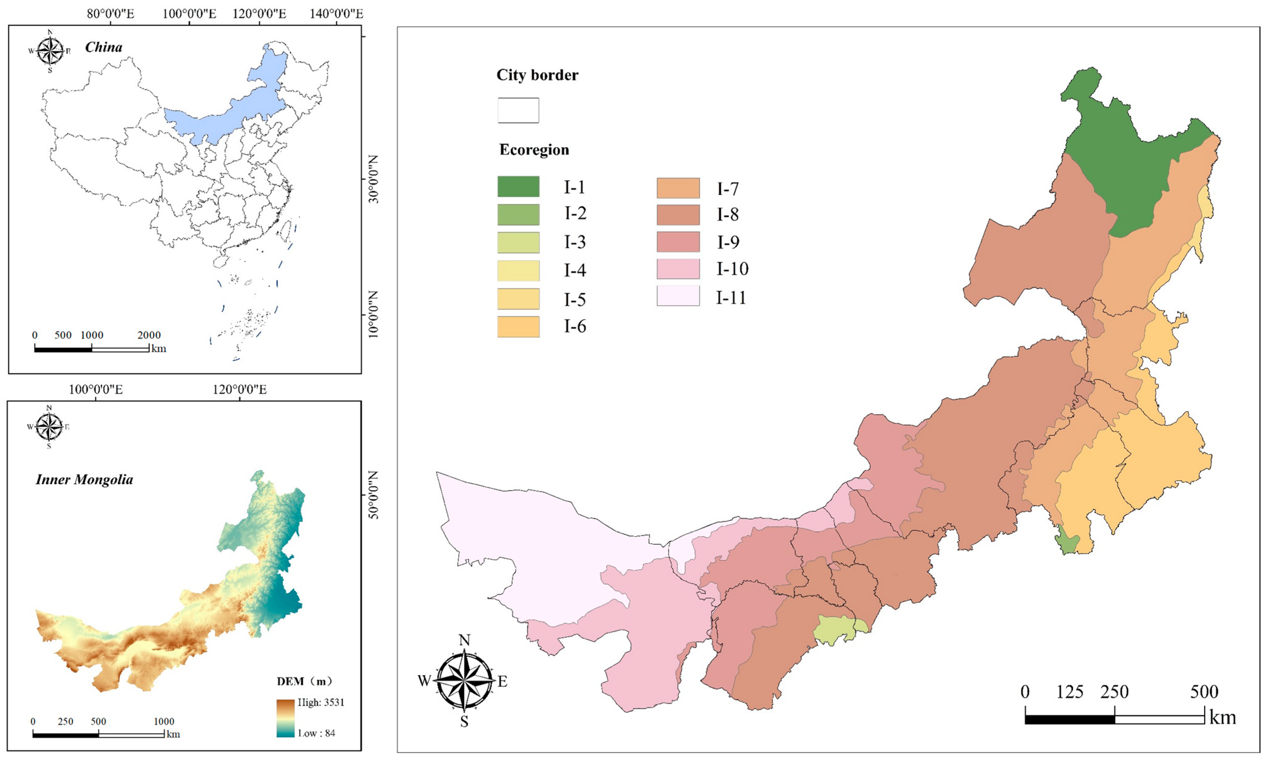
2. Study Area
3. Research Methodology
3.1. Identify Protection Hotspot Areas
3.2. Constructing ST Index for Identifying Hotspot Areas
3.2.1. Interannual Variability Index
3.2.2. Spatial Variability Index
3.3. Construction of Human Footprint Index for Identifying Hotspot Areas
3.3.1. Population
3.3.2. Grazing
3.3.3. Nightlight
3.3.4. Transportation
3.3.5. Land Use
4. Results
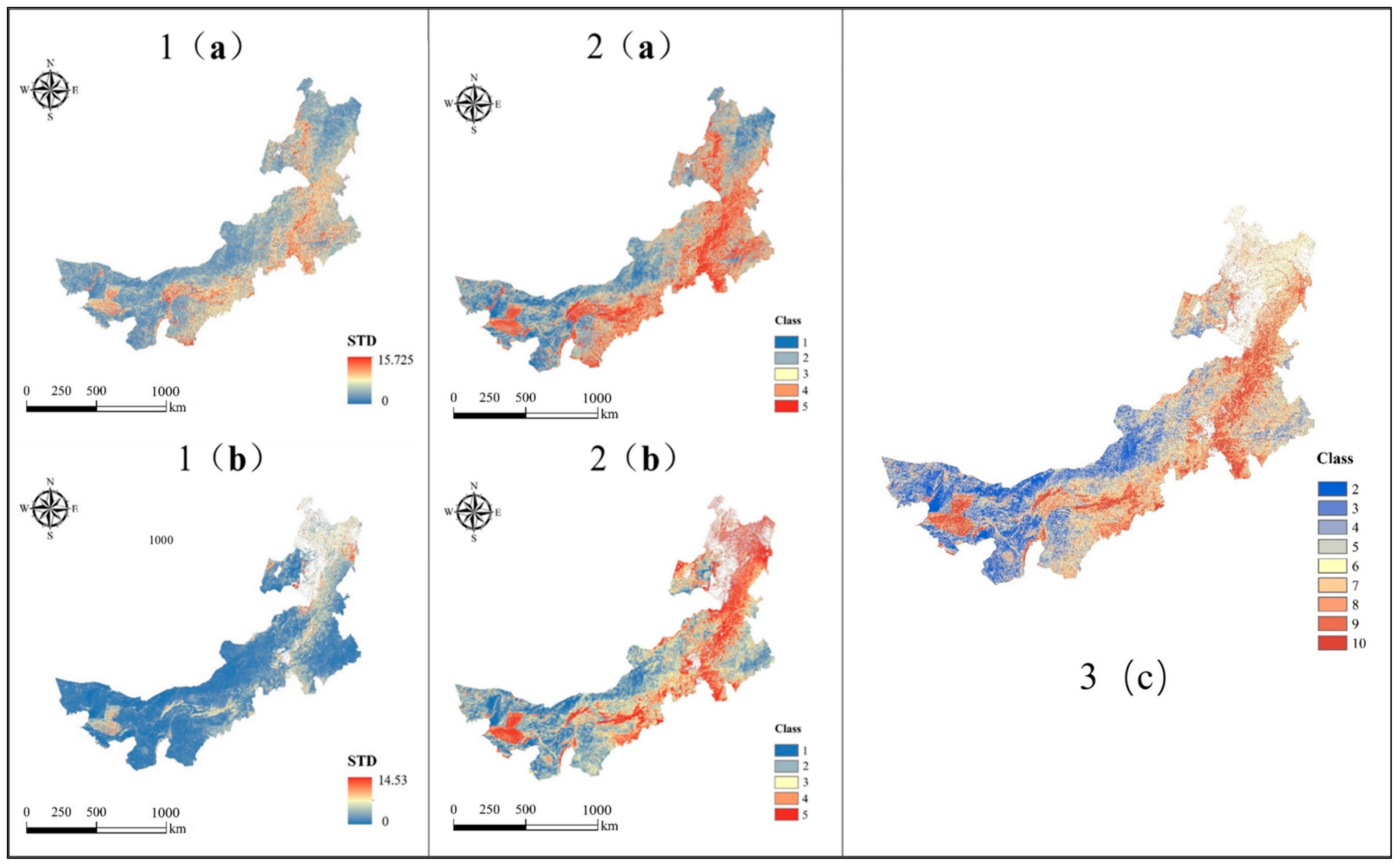
4.1. Spatial–Temporal Remote Sensing Indices to Identify Conservation Areas Affected by Phenological and Seasonal Changes
4.1.1. Interannual Variability of MODIS EVI and LST
4.1.2. Spatial Variability of Landsat 8 EVI and LST Standard Deviation Image Textures
4.1.3. Spatial–Temporal Remote Sensing Index Patterns of the EVI and LST
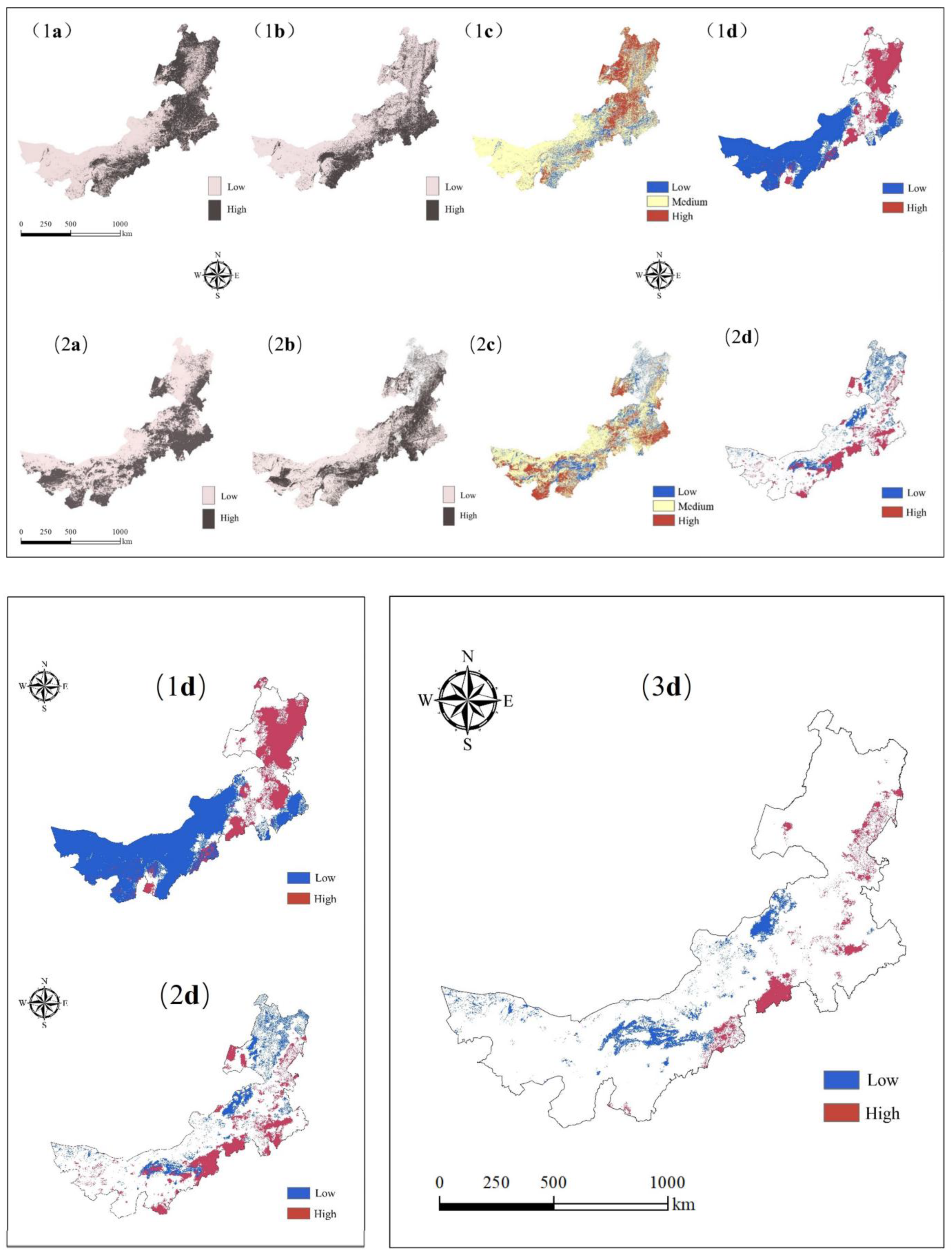
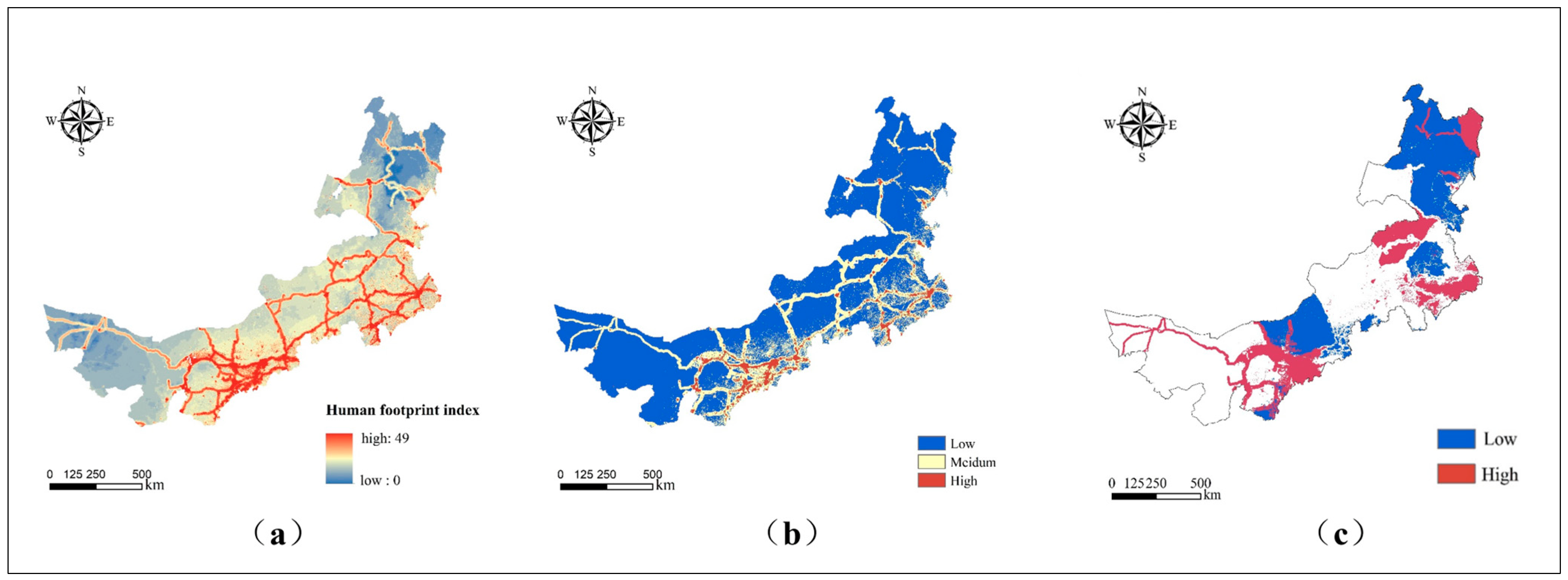
4.2. Human Footprint Index Identifies Conservation Hotspots Affected by Anthropogenic Activities
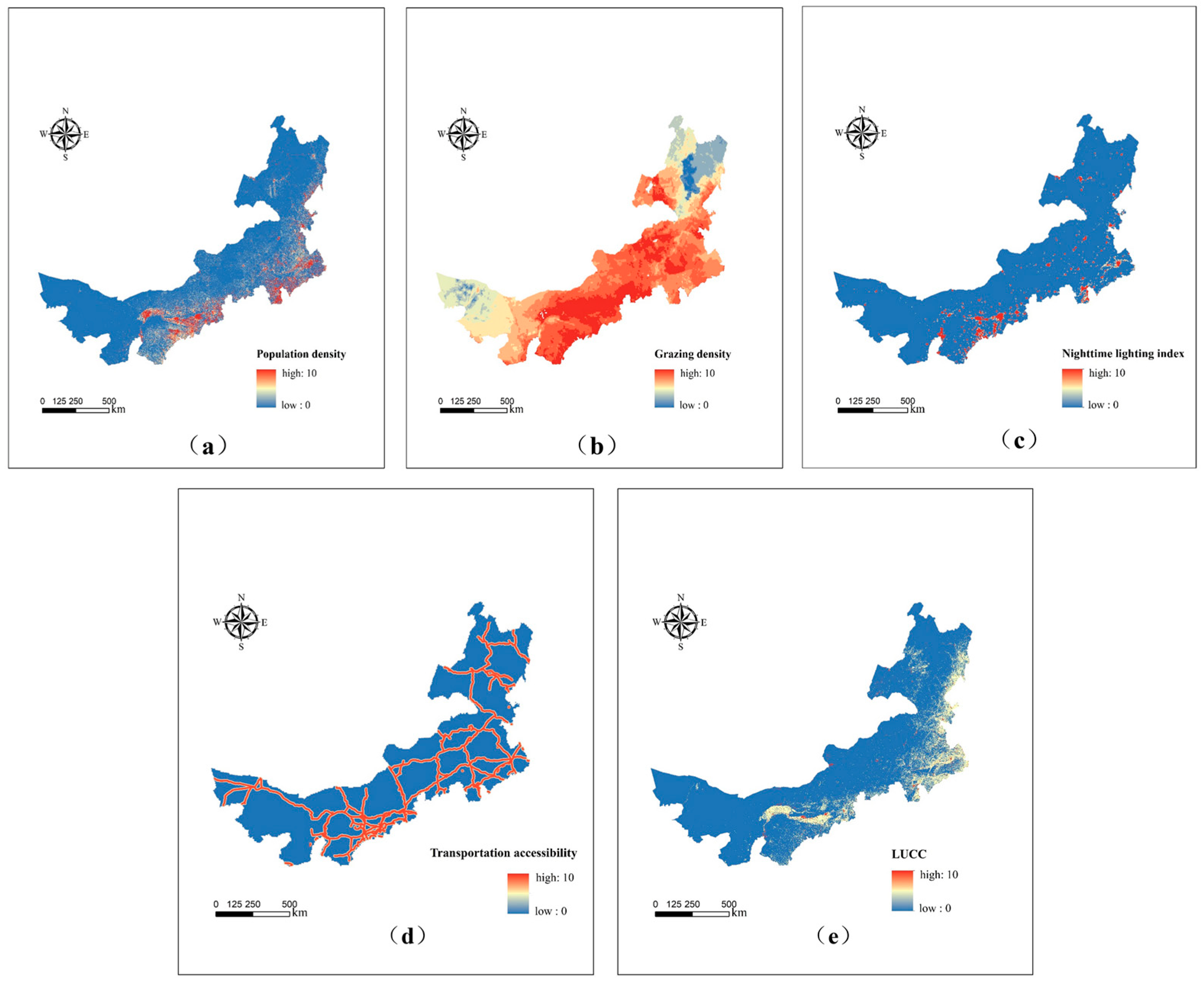
4.2.1. Spatial Distribution of Each Human Activity Factor
4.2.2. Distribution Pattern of Human Footprint Index
4.3. Results of Hotspot Protection Zone Identification
Number, Area, and Spatial Distribution Characteristics of Priority Protected Areas
5. Discussion
5.1. Comparative Analysis of Biodiversity Conservation Hotspot Areas
5.2. Methods for Identifying Hotspot Areas for Biodiversity Conservation
5.2.1. Spatial–Temporal Remote Sensing Index and Biodiversity
5.2.2. Human Footprint Index and Biodiversity
6. Conclusions
Author Contributions
Funding
Institutional Review Board Statement
Data Availability Statement
Conflicts of Interest
References
- Butchart, S.H.M.; Walpole, M.; Collen, B.; van Strien, A.; Scharlemann, J.P.W.; Almond, R.E.A.; Baillie, J.E.M.; Bomhard, B.; Brown, C.; Bruno, J.; et al. Global Biodiversity: Indicators of Recent Declines. Science 2010, 328, 1164–1168. [Google Scholar] [CrossRef]
- Lewis, E.; MacSharry, B.; Juffe-Bignoli, D.; Harris, N.; Burrows, G.; Kingston, N.; Burgess, N.D. Dynamics in the global protected-area estate since 2004. Conserv. Biol. 2019, 33, 570–579. [Google Scholar] [CrossRef] [PubMed]
- Gray, C.L.; Hill, S.L.L.; Newbold, T.; Hudson, L.N.; Borger, L.; Contu, S.; Hoskins, A.J.; Ferrier, S.; Purvis, A.; Scharlemann, J.P.W. Local biodiversity is higher inside than outside terrestrial protected areas worldwide. Nat. Commun. 2016, 7, 12306. [Google Scholar] [CrossRef] [PubMed]
- Larsen, F.W.; Turner, W.R.; Mittermeier, R.A. Will protection of 17% of land by 2020 be enough to safeguard biodiversity and critical ecosystem services? Oryx 2015, 49, 74–79. [Google Scholar] [CrossRef]
- Pimm, S.L.; Jenkins, C.N.; Li, B.V. How to protect half of Earth to ensure it protects sufficient biodiversity. Sci. Adv. 2018, 4, eaat2616. [Google Scholar] [CrossRef] [PubMed]
- Jetz, W.; McGeoch, M.A.; Guralnick, R.; Ferrier, S.; Beck, J.; Costello, M.; Fernandez, M.; Geller, G.N.; Keil, P.; Merow, C.; et al. Essential biodiversity variables for mapping and monitoring species populations. Nat. Ecol. Evol. 2019, 3, 539–551. [Google Scholar] [CrossRef] [PubMed]
- Pereira, H.M.; Leadley, P.W.; Proenca, V.; Alkemade, R.; Scharlemann, J.P.W.; Fernandez-Manjarres, J.F.; Araujo, M.B.; Balvanera, P.; Biggs, R.; Cheung, W.W.L.; et al. Scenarios for Global Biodiversity in the 21st Century. Science 2010, 330, 1496–1501. [Google Scholar] [CrossRef]
- Read, Q.D.; Zarnetske, P.L.; Record, S.; Dahlin, K.M.; Costanza, J.K.; Finley, A.O.; Gaddis, K.D.; Grady, J.M.; Hobi, M.L.; Latimer, A.M.; et al. Beyond counts and averages: Relating geodiversity to dimensions of biodiversity. Glob. Ecol. Biogeogr. 2020, 29, 696–710. [Google Scholar] [CrossRef]
- Zarnetske, P.L.; Read, Q.D.; Record, S.; Gaddis, K.D.; Pau, S.; Hobi, M.L.; Malone, S.L.; Costanza, J.; Dahlin, K.M.; Latimer, A.M.; et al. Towards connecting biodiversity and geodiversity across scales with satellite remote sensing. Glob. Ecol. Biogeogr. 2019, 28, 548–556. [Google Scholar] [CrossRef]
- Wan, X.; Jiang, G.; Yan, C.; He, F.; Wen, R.; Gu, J.; Li, X.; Ma, J.; Stenseth, N.C.; Zhang, Z. Historical records reveal the distinctive associations of human disturbance and extreme climate change with local extinction of mammals. Proc. Natl. Acad. Sci. USA 2019, 116, 19001–19008. [Google Scholar] [CrossRef]
- Thuiller, W.; Lavorel, S.; Araujo, M.B.; Sykes, M.T.; Prentice, I.C. Climate change threats to plant diversity in Europe. Proc. Natl. Acad. Sci. USA 2005, 102, 8245–8250. [Google Scholar] [CrossRef] [PubMed]
- Zhang, Y.; Loreau, M.; He, N.; Wang, J.; Pan, Q.; Bai, Y.; Han, X. Climate variability decreases species richness and community stability in a temperate grassland. Oecologia 2018, 188, 183–192. [Google Scholar] [CrossRef] [PubMed]
- Bongaarts, J. Summary for policymakers of the global assessment report on biodiversity and ecosystem services of the Intergovernmental Science-Policy Platform on Biodiversity and Ecosystem Services. Popul. Dev. Rev. 2019, 45, 680–681. [Google Scholar] [CrossRef]
- Ma, X.; Huete, A.; Yu, Q.; Coupe, N.R.; Davies, K.; Broich, M.; Ratana, P.; Beringer, J.; Hutley, L.B.; Cleverly, J.; et al. Spatial patterns and temporal dynamics in savanna vegetation phenology across the North Australian Tropical Transect. Remote Sens. Environ. 2013, 139, 97–115. [Google Scholar] [CrossRef]
- Mann, M.E.; Park, J. Greenhouse warming and changes in the seasonal cycle of temperature: Model versus observations. Geophys. Res. Lett. 1996, 23, 1111–1114. [Google Scholar] [CrossRef]
- Renner, S.S.; Zohner, C.M. Climate Change and Phenological Mismatch in Trophic Interactions Among Plants, Insects, and Vertebrates. Annu. Rev. Ecol. Evol. Syst. 2018, 49, 165–182. [Google Scholar] [CrossRef]
- Glennon, M.J.; Langdon, S.F.; Rubenstein, M.A.; Cross, M.S. Temporal changes in avian community composition in lowland conifer habitats at the southern edge of the boreal zone in the Adirondack Park, NY. PLoS ONE 2019, 14, e0220927. [Google Scholar] [CrossRef] [PubMed]
- Socolar, J.B.; Epanchin, P.N.; Beissinger, S.R.; Tingley, M.W. Phenological shifts conserve thermal niches in North American birds and reshape expectations for climate-driven range shifts. Proc. Natl. Acad. Sci. USA 2017, 114, 12976–12981. [Google Scholar] [CrossRef] [PubMed]
- Pearce-Higgins, J.W.; Eglington, S.M.; Martay, B.; Chamberlain, D.E. Drivers of climate change impacts on bird communities. J. Ecol. 2015, 84, 943–954. [Google Scholar] [CrossRef]
- Nystrom, M.; Folke, C. Spatial resilience of coral reefs. Ecosystems 2001, 4, 406–417. [Google Scholar] [CrossRef]
- Oliver, T.H.; Heard, M.S.; Isaac, N.J.B.; Roy, D.B.; Procter, D.; Eigenbrod, F.; Freckleton, R.; Hector, A.; Orme, C.D.L.; Petchey, O.L.; et al. Biodiversity and Resilience of Ecosystem Functions. Trends Ecol. Evol. 2015, 30, 673–684. [Google Scholar] [CrossRef]
- Gunderson, L.; Folke, C. Resilience—Now more than ever. Ecol. Soc. 2005, 10, 22. [Google Scholar] [CrossRef]
- Virah-Sawmy, M.; Gillson, L.; Willis, K.J. How does spatial heterogeneity influence resilience to climatic changes? Ecological dynamics in southeast Madagascar. Ecol. Monogr. 2009, 79, 557–574. [Google Scholar] [CrossRef]
- Keppel, G.; Van Niel, K.P.; Wardell-Johnson, G.W.; Yates, C.J.; Byrne, M.; Mucina, L.; Schut, A.G.T.; Hopper, S.D.; Franklin, S.E. Refugia: Identifying and understanding safe havens for biodiversity under climate change. Glob. Ecol. Biogeogr. 2012, 21, 393–404. [Google Scholar] [CrossRef]
- Elsen, P.R.; Farwell, L.S.; Pidgeon, A.M.; Radeloff, V.C. Contrasting seasonal patterns of relative temperature and thermal heterogeneity and their influence on breeding and winter bird richness patterns across the conterminous United States. Ecography 2021, 44, 953–965. [Google Scholar] [CrossRef]
- Hmimina, G.; Dufrene, E.; Pontailler, J.Y.; Delpierre, N.; Aubinet, M.; Caquet, B.; de Grandcourt, A.; Burban, B.; Flechard, C.; Granier, A.; et al. Evaluation of the potential of MODIS satellite data to predict vegetation phenology in different biomes: An investigation using ground-based NDVI measurements. Remote Sens. Environ. 2013, 132, 145–158. [Google Scholar] [CrossRef]
- Hengl, T.; Heuvelink, G.B.M.; Tadic, M.P.; Pebesma, E.J. Spatio-temporal prediction of daily temperatures using time-series of MODIS LST images. Theor. Appl. Climatol. 2012, 107, 265–277. [Google Scholar] [CrossRef]
- Hu, Q.; Sulla-Menashe, D.; Xu, B.; Yin, H.; Tang, H.; Yang, P.; Wu, W. A phenology-based spectral and temporal feature selection method for crop mapping from satellite time series. Int. J. Appl. Earth Obs. Geoinf. 2019, 80, 218–229. [Google Scholar] [CrossRef]
- Farwell, L.S.; Elsen, P.R.; Razenkova, E.; Pidgeon, A.M.; Radeloff, V.C. Habitat heterogeneity captured by 30-m resolution satellite image texture predicts bird richness across the United States. Ecol. Appl. 2020, 30, e02157. [Google Scholar] [CrossRef]
- Wood, E.M.; Pidgeon, A.M.; Radeloff, V.C.; Keuler, N.S. Image Texture Predicts Avian Density and Species Richness. PLoS ONE 2013, 8, e63211. [Google Scholar] [CrossRef]
- Elsen, P.R.; Farwell, L.S.; Pidgeon, A.M.; Radeloff, V.C. Landsat 8 TIRS-derived relative temperature and thermal heterogeneity predict winter bird species richness patterns across the conterminous United States. Remote Sens. Environ. 2020, 236, 111514. [Google Scholar] [CrossRef]
- Strassburg, B.B.N.; Iribarrem, A.; Beyer, H.L.; Cordeiro, C.L.; Crouzeilles, R.; Jakovac, C.C.; Braga Junqueira, A.; Lacerda, E.; Latawiec, A.E.; Balmford, A.; et al. Global priority areas for ecosystem restoration. Nature 2020, 586, 724–729. [Google Scholar] [CrossRef]
- Shrestha, N.; Xu, X.; Meng, J.; Wang, Z. Vulnerabilities of protected lands in the face of climate and human footprint changes. Nat. Commun. 2021, 12, 1632. [Google Scholar] [CrossRef] [PubMed]
- Kennedy, C.M.; Oakleaf, J.R.; Theobald, D.M.; Baruch-Mordo, S.; Kiesecker, J. Managing the middle: A shift in conservation priorities based on the global human modification gradient. Glob. Change Biol. 2019, 25, 811–826. [Google Scholar] [CrossRef] [PubMed]
- Wang, K.; Wang, C.; Feng, X.; Wu, X.; Fu, B. Research progress on the relationship between biodiversity and ecosystem multifunctionality. Acta Ecol. Sin. 2022, 42, 11–23. [Google Scholar]
- Young, H.S.; McCauley, D.J.; Galetti, M.; Dirzo, R. Patterns, Causes, and Consequences of Anthropocene Defaunation. Annu. Rev. Ecol. Evol. Syst. 2016, 47, 333–358. [Google Scholar] [CrossRef]
- Venter, O.; Sanderson, E.W.; Magrach, A.; Allan, J.R.; Beher, J.; Jones, K.R.; Possingham, H.P.; Laurance, W.F.; Wood, P.; Fekete, B.M.; et al. Sixteen years of change in the global terrestrial human footprint and implications for biodiversity conservation. Nat. Commun. 2016, 7, 12558. [Google Scholar] [CrossRef] [PubMed]
- Wei, Q.; Abudureheman, M.; Halike, A.; Yao, K.; Yao, L.; Tang, H.; Tuheti, B. Temporal and spatial variation analysis of habitat quality on the PLUS-InVEST model for Ebinur Lake Basin, China. Ecol. Indic. 2022, 145, 109632. [Google Scholar] [CrossRef]
- Silveira, E.M.O.; Radeloff, V.C.; Martinuzzi, S.; Martinez Pastur, G.J.; Rivera, L.O.; Politi, N.; Lizarraga, L.; Farwell, L.S.; Elsen, P.R.; Pidgeon, A.M. Spatio-temporal remotely sensed indices identify hotspots of biodiversity conservation concern. Remote Sens. Environ. 2021, 258, 112368. [Google Scholar] [CrossRef]
- Correa Ayram, C.A.; Etter, A.; Diaz-Timote, J.; Rodriguez Buritica, S.; Ramirez, W.; Corzo, G. Spatiotemporal evaluation of the human footprint in Colombia: Four decades of anthropic impact in highly biodiverse ecosystems. Ecol. Indic. 2020, 117, 106630. [Google Scholar] [CrossRef]
- Getis, A.; Ord, J.K. The analysis of spatial association by use of distance statistics. Geogr. Anal. 1992, 24, 189–206. [Google Scholar] [CrossRef]
- Clarke, A.; Gaston, K.J. Climate, energy and diversity. Proc. R. Soc. B-Biol. Sci. 2006, 273, 2257–2266. [Google Scholar] [CrossRef]
- Wei, Q.; Halike, A.; Yao, K.; Chen, L.; Balati, M. Construction and optimization of ecological security pattern in Ebinur Lake Basin based on MSPA-MCR models. Ecol. Indic. 2022, 138, 108857. [Google Scholar] [CrossRef]
- Xiao, W.; Lv, X.; Zhao, Y.; Sun, H.; Li, J. Ecological resilience assessment of an arid coal mining area using index of entropy and linear weighted analysis: A case study of Shendong Coalfield, China. Ecol. Indic. 2020, 109, 105843. [Google Scholar] [CrossRef]
- Duan, Q.; Luo, L. A dataset of human footprint over the Qinghai-Tibet Plateau during 1990–2015. China Sci. Data 2020, 5, 303–312. [Google Scholar]
- Wu, Y.; Shi, K.; Chen, Z.; Liu, S.; Chang, Z. Developing Improved Time-Series DMSP-OLS-Like Data (19922019) in China by Integrating DMSP-OLS and SNPP-VIIRS. IEEE Trans. Geosci. Remote Sens. 2022, 60, 1–14. [Google Scholar] [CrossRef]
- Huang, X.; Wu, Z.; Zhang, Q.; Cao, Z.; Zheng, Z.; He, J. Wetland resources distribution and important wetland recognition of Guangdong-Hong Kong-Macao Greater Bay Area based on human pressure index. J. Nat. Resour. 2022, 37, 1961–1974. [Google Scholar] [CrossRef]
- Xu, Y.; Sun, X.; Tang, Q. Human activity intensity of land surface: Concept, method and application in China. Acta Geogr. Sin. 2015, 70, 1068–1079. [Google Scholar] [CrossRef]
- Myers, N. Threatened biotas: “hot spots” in tropical forests. Environmentalist 1988, 8, 187–208. [Google Scholar] [CrossRef] [PubMed]
- Myers, N.; Mittermeier, R.A.; Mittermeier, C.G.; da Fonseca, G.A.B.; Kent, J. Biodiversity hotspots for conservation priorities. Nature 2000, 403, 853–858. [Google Scholar] [CrossRef]
- Dayuan, X. The main content and implementation strategy for China Biodiversity Conservation Strategy and Action Plan. Biodivers. Sci. 2011, 19, 387–388. [Google Scholar] [CrossRef]
- Lamoreux, J.F.; Morrison, J.C.; Ricketts, T.H.; Olson, D.M.; Dinerstein, E.; McKnight, M.W.; Shugart, H.H. Global tests of biodiversity concordance and the importance of endemism. Nature 2006, 440, 212–214. [Google Scholar] [CrossRef]
- Pollock, L.J.; Thuiller, W.; Jetz, W. Large conservation gains possible for global biodiversity facets. Nature 2017, 546, 141–144. [Google Scholar] [CrossRef] [PubMed]
- Orme, C.D.L.; Davies, R.G.; Burgess, M.; Eigenbrod, F.; Pickup, N.; Olson, V.A.; Webster, A.J.; Ding, T.S.; Rasmussen, P.C.; Ridgely, R.S.; et al. Global hotspots of species richness are not congruent with endemism or threat. Nature 2005, 436, 1016–1019. [Google Scholar] [CrossRef] [PubMed]
- Grenyer, R.; Orme, C.D.L.; Jackson, S.F.; Thomas, G.H.; Davies, R.G.; Davies, T.J.; Jones, K.E.; Olson, V.A.; Ridgely, R.S.; Rasmussen, P.C.; et al. Global distribution and conservation of rare and threatened vertebrates. Nature 2006, 444, 93–96. [Google Scholar] [CrossRef] [PubMed]
- Brooks, T.M.; Mittermeier, R.A.; da Fonseca, G.A.B.; Gerlach, J.; Hoffmann, M.; Lamoreux, J.F.; Mittermeier, C.G.; Pilgrim, J.D.; Rodrigues, A.S.L. Global biodiversity conservation priorities. Science 2006, 313, 58–61. [Google Scholar] [CrossRef] [PubMed]
- Margules, C.R.; Pressey, R.L. Systematic conservation planning. Nature 2000, 405, 243–253. [Google Scholar] [CrossRef] [PubMed]
- McIntosh, E.J.; Pressey, R.L.; Lloyd, S.; Smith, R.J.; Grenyer, R. The Impact of Systematic Conservation Planning. Annu. Rev. Ecol. Evol. Syst. 2017, 42, 677–697. [Google Scholar]
- Fourcade, Y.; Engler, J.O.; Roedder, D.; Secondi, J. Mapping Species Distributions with MAXENT Using a Geographically Biased Sample of Presence Data: A Performance Assessment of Methods for Correcting Sampling Bias. PLoS ONE 2014, 9, e97122. [Google Scholar] [CrossRef] [PubMed]
- Jones, M.C.; Cheung, W.W.L. Multi-model ensemble projections of climate change effects on global marine biodiversity. ICES J. Mar. Sci. 2015, 72, 741–752. [Google Scholar] [CrossRef]
- Melo-Merino, S.M.; Reyes-Bonilla, H.; Lira-Noriega, A. Ecological niche models and species distribution models in marine environments: A literature review and spatial analysis of evidence. Ecol. Model. 2020, 415, 108837. [Google Scholar] [CrossRef]
- Hikosaka, K.; Ishikawa, K.; Borjigidai, A.; Muller, O.; Onoda, Y. Temperature acclimation of photosynthesis: Mechanisms involved in the changes in temperature dependence of photosynthetic rate. J. Exp. Bot. 2006, 57, 291–302. [Google Scholar] [CrossRef]
- An, S.; Zhu, X.; Shen, M.; Wang, Y.; Cao, R.; Chen, X.; Yang, W.; Chen, J.; Tang, Y. Mismatch in elevational shifts between satellite observed vegetation greenness and temperature isolines during 2000–2016 on the Tibetan Plateau. Glob. Change Biol. 2018, 24, 5411–5425. [Google Scholar] [CrossRef]
- Liu, H.; Zhang, M.; Lin, Z.; Xu, X. Spatial heterogeneity of the relationship between vegetation dynamics and climate change and their driving forces at multiple time scales in Southwest China. Agric. For. Meteorol. 2018, 256, 10–21. [Google Scholar] [CrossRef]
- Wang, J.; Meng, J.J.; Cai, Y.L. Assessing vegetation dynamics impacted by climate change in the southwestern karst region of China with AVHRR NDVI and AVHRR NPP time-series. Environ. Geol. 2008, 54, 1185–1195. [Google Scholar] [CrossRef]
- Zeng, L.; Wardlow, B.D.; Xiang, D.; Hu, S.; Li, D. A review of vegetation phenological metrics extraction using time-series, multispectral satellite data. Remote Sens. Environ. 2020, 237, 111511. [Google Scholar] [CrossRef]
- Liu, Y.; Wu, C.; Peng, D.; Xu, S.; Gonsamo, A.; Jassal, R.S.; Arain, M.A.; Lu, L.; Fang, B.; Chen, J.M. Improved modeling of land surface phenology using MODIS land surface reflectance and temperature at evergreen needleleaf forests of central North America. Remote Sens. Environ. 2016, 176, 152–162. [Google Scholar] [CrossRef]
- Guette, A.; Godet, L.; Juigner, M.; Robin, M. Worldwide increase in Artificial Light At Night around protected areas and within biodiversity hotspots. Biol. Conserv. 2018, 223, 97–103. [Google Scholar] [CrossRef]
- Feng, C.-T.; Cao, M.; Liu, F.-Z.; Zhou, Y.; Du, J.-H.; Zhang, L.-B.; Huang, W.-J.; Luo, J.-W.; Li, J.-S.; Wang, W. Improving protected area effectiveness through consideration of different human-pressure baselines. Conserv. Biol. 2022, 36, e13887. [Google Scholar] [CrossRef] [PubMed]
- Wei, W.; Swaisgood, R.R.; Pilfold, N.W.; Owen, M.A.; Dai, Q.; Wei, F.; Han, H.; Yang, Z.; Yang, X.; Gu, X.; et al. Assessing the Effectiveness of China’s Panda Protection System. Curr. Biol. 2020, 30, 1280.e2–1286.e2. [Google Scholar] [CrossRef] [PubMed]
- Spear, D.; Foxcroft, L.C.; Bezuidenhout, H.; McGeoch, M.A. Human population density explains alien species richness in protected areas. Biol. Conserv. 2013, 159, 137–147. [Google Scholar] [CrossRef]
- Venter, O.; Sanderson, E.W.; Magrach, A.; Allan, J.R.; Beher, J.; Jones, K.R.; Possingham, H.P.; Laurance, W.F.; Wood, P.; Fekete, B.M.; et al. Global terrestrial Human Footprint maps for 1993 and 2009. Sci. Data 2016, 3, 160067. [Google Scholar] [CrossRef]


| High Spatial Variability | Low Spatial Variability | |
|---|---|---|
| High interannual variability | Medium conservation (high interannual variability poses a high threat but high spatial variability in EVI and LST implies high resilience) | Highest conservation (high interannual variability poses high threat; low spatial variability in EVI and LST means low resilience and low elasticity) |
| Low interannual variability | Lowest conservation (low interannual variability poses low threat level; high spatial variability in EVI and LST implies high resilience) | Medium conservation (low interannual variability poses low threat level; low spatial variability in EVI and LST implies low resilience) |
| Phenology and Seasonal Indicators | Description | Interannual Variability Index |
|---|---|---|
| Esos | Start of the growing season based on EVI timeseries | _ Es |
| Eeos | End of the growing season calculated from EVI timeseries | _ Ee |
| Elos | Number of days between EVI start date and end date | _ El |
| Lsos | Start of the growing season based on LST timeseries | _ Ls |
| Leos | End of the growing season calculated from LST timeseries | _ Le |
| Llos | Number of days between LST start date and end date | _ Ll |
| Priority Zone Level | Climate Change Threatening | Human Activities Threatening |
|---|---|---|
| Primary Protection Priority Area (A1–A12) | High | High |
| Secondary Protection Priority Area | High | Low |
| Low | High | |
| Tertiary Protection Priority Area | Low | Low |
| First-Class Protection Priority Area Name (A1–A12) | District | Regional Details |
|---|---|---|
| A1 Dobao Shan Town Nature Reserve | Heihe City, Dobao Shan Town | There are 1880 km2 of woodland in Dobao Shan town, with 19,457,600 cubic meters of standing wood, mainly larch, poplar, linden, Quercus, and birch. The vegetation cover is high and the biodiversity is outstanding, most of the area is in a natural wild state. |
| A2 Molidawa Bayan Wetland Ecosystem Reserve | Hulunbuir City, Molidawa Daur autonomous Banner, Bayan Ewen National Township | Molidawa Bayan National Wetland Park has a wetland area of 30,168 km2, bringing together a number of regional biota compositions such as the Daxinganling, Mongolian Plateau, Songliao Plain, Changbai Mountain, and North China in China, and has outstanding biodiversity. |
| A3 (a) Wildlife Nature Reserve in southeastern Chabach Township | (a) Hulunbuir City, Arrong Banner, Chabach Ewenke National Township | The area under the jurisdiction of Chabach Township is 164 km2 of arable land, 370 km2 of forest land, and 186.67 km2 of pasture. Rich forestry resources, large areas of forests provide living conditions for wild animals, mainly moose, horse deer, brown bear, roe deer, wild boar, lynx, snow rabbits, pheasants, flying dragons, and other wild animals. |
| A3 (b) Forest Ecosystem and Wildlife Reserve in the South of Zalantun, Wolniuhe Township | (b) Hulunbuir City, Arong Banner, Woliuhe Town, | Wolniuhe Town has 1.054 km2 of forest, 75.27% forest coverage, and 186.67 km2 of pasture. The territory has abundant water resources, fertile land and mild climate. There are wild plants and herbs such as mushroom, fern, yellow flowering cabbage, monkey fungus, hazelnut, etc. There are also many kinds of wild animals protected by the state such as mountain rabbit, wild boar, roe deer, wild song, flying dragon, etc. |
| A4 (a) Mengelhan Mountain Nature Reserve * | Hinggan League, Horqin Right Wing Banner, Ulanmadu Sumxiang | Mengelhan Mountain Nature Reserve, a provincial-level nature reserve, is located at the South of the Daxinganling Mountains and in the northern part of Horqin Grassland. Its total area is 212.17 km2. The main objects of protection are natural secondary forests, grassland meadow ecosystems, and rare wildlife and plants. |
| A4 (b) Ulan River Nature Reserve * | Hinggan League, Horqin Right Wing Banner. | Ulan River Nature Reserve is a provincial-level nature reserve. The total area is 585.15 km2 and the main protection object is the water-conserving forest. |
| A5 Bayanhusumxiang Central Grassland Ecosystem Reserve | Xilin Gol league, West Ujimqin Banner, Bayanhu shumxiang. | With a total area of more than 70,000 km2, the Urumqi grassland has been designated as a “National Key Ecological Function Area”. |
| A6 Baoligeng Northeast Grassland Ecosystem Reserve | Chifeng City, Xilinhot City Baoligansumu. | Baoligansumu is part of the Inner Mongolia Plateau and has a complete grassland type, namely meadow grassland, typical grassland, semi-desert grassland, and sandy grassland, with more than 1200 kinds of plants on the ground. |
| A7 (a) South-central Balach Ruud Sumu Grassland Ecosystem Reserve | Chifeng City, Aruqorchin Banner, Barachilde South Central | The northern part of Balachi Zhongde is dominated by the reforestation of barren hills and the southern part is dominated by the great reforestation of Wanli, with a construction area of more than 200 km2. |
| A7 (b) Xiaoheyan Autonomous Region-level Wetland Bird District Nature Reserve * | Chifeng City, Aohan Banner, Linxi Town, | With a total area of 180 km2, the Xiaoheyan Autonomous Region Wetland Bird Nature Reserve is a comprehensive nature reserve that focuses on protecting birds and the wetland ecosystem on which they depend. |
| A8 Saiyinghuduga Sumu Northwest Grassland Ecosystem and Wildlife Reserve | Xilin Gol league Zhenglan banner, SaiyinHuduga Sumu | Saiyinghuduga Sumu is rich in wildlife resources, with 708 kinds of plants and more than 20 kinds of rare wildlife resources. |
| A9 (a) Forest Ecosystem Reserve in Uduntauhai Town | Chifeng City, Wunniut Banner, Wuduntauhai Town | The town has a forest area of 190 km2, with a forest coverage rate of 37%. The tree species are poplar, almond, elm, camphor pine, fruit trees, etc. |
| A9 (b) Wupaizi Nature Reserve * | Chifeng City, Wunniut Banner, Wupaizi Village | The reserve covers an area of about 8 km2 and is a protected area for wetland ecosystems and rare birds. |
| A10 (a) Black Tiger Mountain-Eagle Beak Mountain Wildlife Nature Reserve * | Hohhot City, Qingshuihe County, Beibao Township | The reserve covers a total area of 3 km2 and the main objects of protection are mountain forests, scrub ecosystems, and wild plants and animals. |
| A10 (b) Qingshuihe County Shake Forest Gorge Nature Reserve * | Hohhot City, Qingshuihe County, Leekzhuang Township | With a total area of 51.7 km2, the reserve is a comprehensive nature reserve with a variety of ecosystems such as mountain forests and thickets; rare wildlife and plants are the main objects of protection. |
| A10 (c) Baiji Shaba Nature Reserve * | Hohhot City, Linge County | Baiji Shaba Nature Reserve is a nationally known example of successful sand control and reforestation. The type of protection belongs to desert ecosystem and wildlife reserve. |
| A11 Ortok Banner Licorice Nature Reserve * | Erdos City, Ortoge Banner | The total area of the reserve is 1448 km2. It is a nature reserve for wild plant types and protects endangered wild plant populations represented by Ural licorice and fragile desert steppe ecosystems and their biodiversity. |
| A12 (a) Shanghai Miao Town Western Licorice Nature Reserve | Erdos City, Ortok Qianqi Banner, Shanghai Miao Town | Shanghai Miao town is in the southwest of Ertok former banner, planting valuable the medicinal herbs including licorice (453.33 km2) with high quality; wild medicinal herbs also include wintergreen, bitter ginseng, white tribulus terrestris, free silk, motherwort, and so on. The town can use 3280 km2 of pasture, of which 1000 km2 is for the rare plant species Tibetan broccoli. |
| A12 (b) Olezaki Town Central Dashatou Desert Nature Reserve | Erdos City, Ortok Qianqi Banner, Olezhaoqi Town | This is a typical combination of agricultural and pastoral lands. The natural resources in the area mainly include Tibetan broccoli, licorice outside Liang, ephedra, gypsum, natural gas, oil, etc. |
Disclaimer/Publisher’s Note: The statements, opinions and data contained in all publications are solely those of the individual author(s) and contributor(s) and not of MDPI and/or the editor(s). MDPI and/or the editor(s) disclaim responsibility for any injury to people or property resulting from any ideas, methods, instructions or products referred to in the content. |
© 2023 by the authors. Licensee MDPI, Basel, Switzerland. This article is an open access article distributed under the terms and conditions of the Creative Commons Attribution (CC BY) license (https://creativecommons.org/licenses/by/4.0/).
Share and Cite
Lu, Y.; Wang, H.; Zhang, Y.; Liu, J.; Qu, T.; Zhao, X.; Tian, H.; Su, J.; Luo, D.; Yang, Y. Combining Spatial–Temporal Remote Sensing and Human Footprint Indices to Identify Biodiversity Conservation Hotspots. Diversity 2023, 15, 1064. https://doi.org/10.3390/d15101064
Lu Y, Wang H, Zhang Y, Liu J, Qu T, Zhao X, Tian H, Su J, Luo D, Yang Y. Combining Spatial–Temporal Remote Sensing and Human Footprint Indices to Identify Biodiversity Conservation Hotspots. Diversity. 2023; 15(10):1064. https://doi.org/10.3390/d15101064
Chicago/Turabian StyleLu, Yuting, Hong Wang, Yao Zhang, Jiahao Liu, Tengfei Qu, Xili Zhao, Haozhe Tian, Jingru Su, Dingsheng Luo, and Yalei Yang. 2023. "Combining Spatial–Temporal Remote Sensing and Human Footprint Indices to Identify Biodiversity Conservation Hotspots" Diversity 15, no. 10: 1064. https://doi.org/10.3390/d15101064