Article

Variation in Plant Diversity along a Watershed in the Semi-Arid Lands of North Africa

1
Water and Environment Laboratory, Larbi Tebessi University, Tebessa 12000, Algeria
2
Laboratory of Plant Biology, Department Biology of Living Beings, Faculty of Exact Sciences and Nature and Life Sciences, Larbi Tebessi University, Tebessa 12002, Algeria
3
Biomolecules and Application Laboratory, Faculty of Exact Sciences and Nature and Life Sciences, Larbi Tebessi University, Tebessa 12002, Algeria
4
Department of Forest Management, Higher National School of Forests, Khenchela 40000, Algeria
5
Laboratory of Natural Resources and Management of Sensitive Environments ‘RNAMS’, University of Oum-El-Bouaghi, Oum-El-Bouaghi 04000, Algeria
*
Author to whom correspondence should be addressed.
Diversity 2022, 14(6), 450; https://doi.org/10.3390/d14060450
Submission received: 19 January 2022 / Revised: 4 April 2022 / Accepted: 23 May 2022 / Published: 2 June 2022

Abstract

:
Plants are a vital part of the world’s biological diversity and have great economic and cultural importance. Plant biodiversity balances ecosystems, protects watersheds, mitigates erosion, affects climate, and provides shelter for many animal species. This study aimed to determine plant diversity in relation to the soil properties of semi-arid rangelands along a gradient at the watershed scale in the Oued Chabro, Algeria. Plants and soil were sampled at 27 points distributed in three sampling sites (upstream, midstream, and downstream). The floristic data was analyzed using species richness estimators, life forms, spatial occurrence, and multiple factor analysis. Moreover, the effects of soil properties on the taxonomic structure of plant communities in the sampling sites were analyzed using Pearson correlations. The characterized flora included 42 plant species classified into 18 families, and Asteraceae (38.1%), Poaceae (14.3%), Brassicaceae (7.1%), Amaranthaceae (4.8%), and Chenopodiaceae (4.8%) were the most representative in terms of species. The species Atractylis delicatula was dominant (relative abundance = 81.5%). The upstream site was characterized by a high vegetation cover, high species abundances, and richness in plant families and genera. Significant correlations were observed in this area between the number of genera, number of families, number of species, family richness, Pielou evenness index, and Simpson’s concentration index. The upstream site was characterized by chamaephytes and phanerophytes; 16 species were exclusively present in this section. Two species were found in the midstream site and one (Scolymus hispanicus) was found in downstream site. The upstream site was positively correlated with plant litter, the midstream with barren soil, and the downstream study area was negatively correlated with coarse-grained materials and vegetation cover. This study demonstrated that differences in life forms, richness, and diversity exist among the three sampling sites due to the soil differences and the positions along the watershed.

1. Introduction

North African wadis (or oueds) are intermittent rivers and streams that occur in areas with limited water resources. In the context of climate change, the poor management of freshwater exacerbates the growing local demand for this precious resource, which may amplify the current water deficit [1,2]. Algeria has multiple natural wetlands with high diversity resulting from plant formations with a high species richness and different structures and landforms. The country presents a great climatic diversity—as all the Mediterranean bioclimatic stages, from humid to Sahara, are met there—which gives its regions high value for animal and plant diversity [3].
Vegetation cover constitutes a fundamental component of ecosystems and provides several services to the livelihood community [4]. Vegetation can be used as an indicator, providing information about habitat conditions and helping to determine the direction of changes in these conditions [5]. Changes in structure and plant communities also contribute to understanding environmental factors and their associated impacts [4]. Ecological attributes related to vegetation cover structure, such as perennial and annual species density and species diversity, are important indicators of environmental disturbances [6].
It can be expected that the regulation of plant distribution in rivers will take place from whole stream systems to stream discharges and habitats within stream reaches. Plant species are subsequently influenced by the environmental conditions within the river reach, when it successfully arrives and establishes at a certain stream site. It has been previously found that the distribution of plants at the spatial scale of the river reach is related to alkalinity, river size, and the occurrence of coarse substrate in Danish streams [7]. The river continuum concept (RC concept) predicts that the highest number of species will be found in medium-sized rivers with moderate disturbance, high physical heterogeneity, and favorable lighting and sedimentary conditions, while the species number will be lower in the upstream and downstream sections with unfavorable light and sediment conditions [8].
Arid and semi-arid environments offer opportunities for the evaluation and understanding of the mechanisms involved in the diversification and adaptation of plants in relation to the evolution of their environment [9]. The relationships between environmental factors and vegetation have attracted great interest in recent decades, and many studies have explored the relationship between soil and floristic factors [10,11,12]. In arid or semi-arid ecosystems, plant population dynamics and community properties are controlled by abiotic factors [13], while in moister environments with less precipitation variation, plant community properties are more directly controlled by grazing [14].
Nevertheless, the hydrogeographic context of northeastern Algeria is poorly studied. A taxonomic list of spontaneous vegetation is unknown for most watersheds and wadis. Therefore, this study provides a list of natural flora from a permanent wadi (Chabro Wadi) of northeast Algeria. The aims of the study were to: (i) examine the botanical composition, including the plant richness, plant diversity, taxonomical structure, and diversity of life forms; (ii) determine the influence of soil physicochemical properties on plant distribution along the watershed; and (iii) determine the relationship between soil physicochemical properties and plant species found within the vegetation patches on Chabro Wadi.

2. Materials and Methods

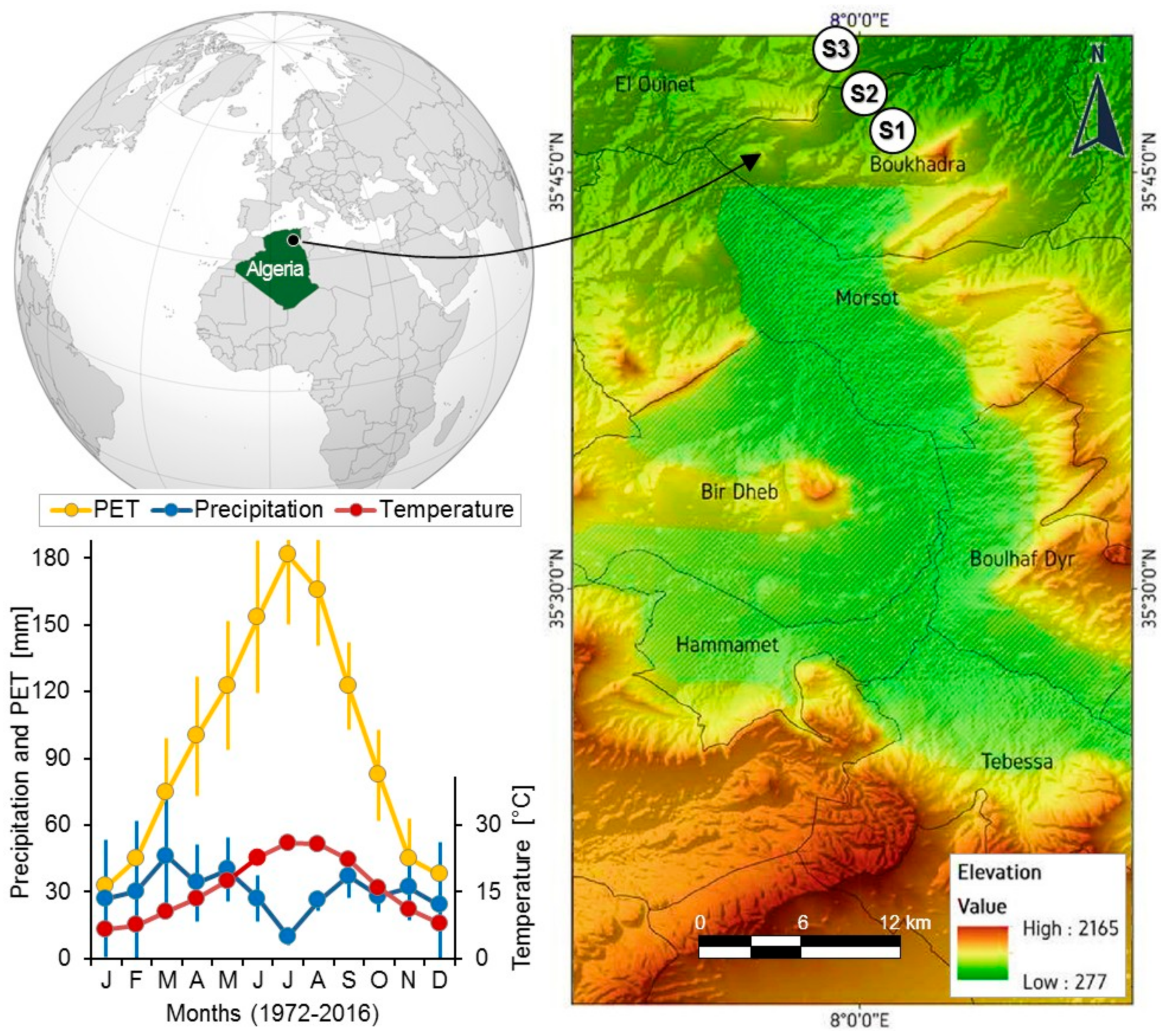
2.1. Study Area and Sampling Sites

The study area is part of the Tebessa Province (wilaya) in northeastern Algeria; it stretches within the northern latitudes of 35°10′ to 35°22′ and the eastern longitudes of 7°13′ to 7°55′, which covers about ~13,261 km2. This wilaya is limited to the north by Souk Ahras, to the south by El Oued, to the west by Constantine, and to the east by the Algeria–Tunisia border (Figure 1). An analysis of climate data from 2020 provided by InfoClimat (www.infoclimat.fr, 22 December 2021) and Tutiempo (https://tutiempo.net, 22 December 2021) indicated that annual precipitation during the study period totaled 369.2 mm, with a maximum in September (78.2 mm) and a minimum in August (0 mm). The average annual temperature is 23.64 °C, with a maximum in July (35.3 °C) and a minimum in December (8.4 °C). According to the Köppen classification, the climate is BSK (i.e., a dry and cold semi-arid steppe climate) [15]. The aridity index of De Martonne (1926) is 14.30, indicating a semi-arid climate. The Gaussen and Bagnouls diagram shows a dry season that lasts more than five months a year, from mid-May to late October (Figure 1). Three stations were sampled through the study area: (i) station 1 (8.09°98′57″ E, 35.44°70′64″ N) was located upstream of the oued; (ii) station 2 (8.04°28′81″ E, 35.49°41′15″ N) at the center of the oued; and (iii) station 3 (7.98°21′49″ E, 35.63°87′24″ N) downstream from the oued.

2.2. Sampling Plants

In the same plots where we collected soil samples, we also collected data on the vegetation. The monitoring of plants was conducted during the optimal growing period (February to April 2021). The choice of sample locations was random and took into account the apparent homogeneity of the vegetation of the region. The sampling area of each sample was 100 m2. This area is commonly applied for sampling the vegetation of Algerian steppe rangelands [16]. The number of sampling points was about nine quadrants per station (a total of 27 quadrants distributed throughout 3 stations); the vegetation represented was quantified in 100 m2 quadrants (10 × 10m) along the station. The observations were marked at regular intervals of 10 cm (100 points) along the line transect. The distance between a quadrant and the following quadrant was 10 m. All plants that intercepted transects were identified and registered. Inside each plot, plant species were identified, and their nomenclature was adopted according to the flora of Algeria [17,18].
At each sampling site, 27 soil samples were collected using an auger at an average depth of 20–30 cm. Soil sampling was carried out within the same area used to sample vegetation. In this plot, soil samples were randomly collected, then all the subsamples were mixed to create a single composite soil sample that was analyzed in the lab. In the laboratory, physical and chemical analyses were carried out on the fine earth that was air-dried and sieved at Ø < 2 mm. Soil pH and electrical conductivity (EC) were measured at 1:5 soil–water suspension ratios. Organic carbon (SOC) was determined using Anne’s method [19] by the oxidation of carbon with excess potassium dichromate (K2Cr2O7) in sulfuric acid medium (heat source). The amount of non-consumed dichromate was measured back by Mohr’s salt. The rate of organic matter (OM) was estimated by multiplying the percentage of carbon by 1.72 [20]. Subsequently, the granulometric composition of each sample was determined according to PN ISO 11277:2005 as a fraction of stones (>75 mm), gravel (2–75 mm), sand (0.05–2 mm), or silt (<0.05 mm).

2.3. Evaluation of Plant Cover, Occurrence, and Life forms

Plant cover is an important ecological feature that refers to the amount of ground surface covered by plants and can be estimated using the following formula [21]:
C o v e r   % = i = 1 n n u m b e r   o f   h i t s   o f   s p e c i e s   n T o t a l   n u m b e r   o f   p o i n t s × 100
Using the same technique, i.e., LIT, as we did for computing vegetation cover, we determined soil-surface covers (in %) for plant litter, coarse-grained materials, and bare ground. For each plant species, occurrence (%) was computed as the number sampling points were the species occurred divided by the total number of points per sampling site. In addition, the plants were categorized using the life forms of the Raunkiær system, which were used as proxies of plant functional traits.

2.4. Alpha and Beta Diversity, Rarefaction, and Interpolation of Species Richness

The diversity of plants in the sampling sites was evaluated the using vegetation cover, relative frequency (RF) of species, Hill numbers, and Pielou evenness index (E). Relative frequency provides information on the rate of occurrence of a species along a transect for each cell [22]. It can be calculated using the following formula [23]:
R F = number   of   occurences   of   species Total   number   of   occurences   of   all   species × 100
Diversity was estimated using Hill numbers (qD) expressed by Hill’s q-metrics, with qD: D q = ( i = 1 s P i q ) 1 / 1 q . The parameter q controls the sensitivity of this diversity estimate to species’ relative frequencies (Pi): (i) for q = 0, this index (0D) is simply S (species richness), where all species are given equal weight; (ii) when q tends to 1, the index 1D expresses the exponential of Shannon’s index (H’), and greater weight is given to common species; and (iii) for q = 2, the index 2D yields becomes the inverse of Simpson’s concentration index (D) where greater weight is given to dominant species [24].
The Pielou evenness index (E) measures the distribution of species within a transect, regardless of the species richness [25].
Species richness estimates were carried out using the EstimateS program [26]. Four asymptotic richness estimators were applied—Chao1 and Chao2 richness estimators (S(Chao1) and S(Chao2)) and the first- and second-order jackknife estimators (S(Jack1) and S(Jack2)):
S Jack 1 = S obs + Q 1 m 1 m
S Jack 2 = S obs + Q 1 2 m 3 m Q 2 m 2 2 m m 1
s C h a o 1 = s o b s + n 1 n × F 1 F 1 1 2 F 2 + 1
S C h a o 2 = S o b s + m 1 m × Q Q 1 1 2 Q 2 + 1
where Q1 represents uniques, Q2 is duplicates, F1 is singletons, F2 is doubletons, m is sample size, n is the number of individuals. The estimates of species richness were obtained following 100 randomizations and given as means ± SD.
In order to define if the sampling effort applied at each sampling site was sufficient to encounter all plant species, we carried out species richness interpolation via species accumulation curves. For each sampling site, as well as the whole Chabro Wadi, interpolations were performed 9 times the reference sampling size that was nine relevés per site and 27 for the three sites combined.
Beta diversity was determined using the EstimateS software. The similarity of species richness between sampling site plant groups was analyzed using several similarity indices in order to obtain a comprehensive analysis, which was complemented with a Venn diagram. A similarity analysis was carried out using qualitative-based and qualitative-based indexes including the Jaccard, Sørensen, Morisita–Horn, and Bray–Curtis indexes [24,27].

2.5. Taxonomic Diversity

First, the relative frequencies of species per family were determined for the total inventory. In each sampling unit, the genus or family richness to species richness ratios (G/S or F/S ratio) were computed. In former studies, the taxonomic structure has been demonstrated to vary between spatial and temporal sampling units. The relationships between generic or family richness and species richness (species–higher taxon relations) were analyzed using these models [28,29]:
ln(G) = a + b × ln(S) and ln(F) = a + b × ln(S)
where G represents the number of genera, F is the number of families, and S is the number of species. The intercept parameter a of the previous two models was set to 0 because of the taxonomic structure where each species belongs only to one genus and one family. Accordingly, the forms of the models used were ln(G) = b × ln(S) for the species–genus relationship and ln(F) = b × ln(S) for the species–family relationship. Regression analysis was used to estimate the exponent of b in the species–higher taxon relationship.

2.6. Data Management and Statistical Analysis

For each sampling site within the Chabro watershed, soil data and plant diversity traits were summarized using descriptive statistics, viz., mean, range (min–max), standard deviation (SD), median (Med), and the coefficient of variation (CV). These statistics of plant diversity indices were represented in boxplot form to facilitate comparisons between sampling sites. When the CV is less than 10%, the data expresses low variability, while it demonstrates high variability when the CV is greater than 90% [30,31]. The variation of the same indices among sampling sites was tested using generalized linear models (GLMs). Shapiro–Wilk tests were applied to verify the normality of the data. The variation of G/S and F/S ratios among sampling sites was tested using one-way ANOVA. Significance tests (p < 0.05) were processed further using Tukey’s HSD post hoc test. For each sampling site, Pearson correlation tests were applied between soil characteristics (physicochemical properties and surficial covers) and G/S and F/S ratios. Correlation tests were carried out between diversity parameters in order to explore the relationships between plant diversity indices.
A multiple factor analysis was performed in order to distinguish between the plant and abiotic characteristics of the three scales (down-, mid-, and upstream) of the Chabro watershed. All the measured data were included in the same analysis. The variables measured at each sampling site were grouped in into six categories, including (i) soil-surface covers with four inputs (plant litter, coarse-grained materials, barren soil, and total vegetation cover); (ii) soil physicochemical properties with eight inputs (pH, EC, OM, SOC, gravel, sand, silt, and clay); (iii) plant lifeforms with five inputs (chamaephytes, geophytes, hemicryptophytes, phanerophytes, and therophytes; (iv) taxonomic structure with 5 inputs (#Families, #Genera, #Species, G/S ratio, and F/S ratio); (v) taxonomic diversity with 6 inputs (S, N, H, E, D, and D:S ratio); (vi) richness estimates with 8 inputs (S(Chao1), S(Chao2), S(Jack1), S(Jack2), S(Bootstrap) (bootstrap richness estimator), S(MM) (Michaelis–Menten richness estimator), ACE (abundance coverage-based estimator), and ICE (incidence coverage-based estimator)). For each of the above categories, a principal component analysis (PCA) was obtained based on the inputs of the specific variable. The free software R was used to carry out the statistical analyses.

3. Results

3.1. Soil Characteristics of Vegetation Types

The results of the soil physicochemical analysis and soil-surface characteristics are shown in Table 1. The coefficient of variation (CV) values were between 0.10 and 0.90, except for those of silt and clay. This indicated that the plant litter, coarse materials, bare soil, pH, electrical conductivity (EC), organic matter (OM), soil organic carbon (SOC), sand, and gravel had moderate variability, while the silt (CV = 187%) and clay (CV = 131%) had great variability in the study area. The downstream site was characterized by a vegetation cover ranging between 43 and 67%; it varied between 19% and 34% at the midstream site and from 45 to 82% at the upstream site. With regard to OM content, the studied soils were generally classified as low in OM (0.28% to 1.45%). We observed a spatial variation in OM content, which was directly related to shifts in vegetation cover. However, this variation was not statistically significant.

3.2. Floristic Composition

The floristic inventory for our watershed scale included 42 plant species belonging to 41 genera and 18 different families from 2942 individuals (Table 2). The most widely represented families were Asteraceae (38.10%), Poaceae (14.29%), Brassicaceae (7.14%), Amaranthaceae, and Chenopodiaceae (4.76%), whereas the majority of the other families were represented by only one species.
The family Asteraceae was the best represented with 1013 individuals and sixteen species, compared to Poaceae with 624 individuals and six species. The species of Asteraceae with the highest relative abundances (RAs) were Atractylis delicatula L. (81.5%), Carduncellus pinnatus Desf. (70.4%), Calendula arvensis L. (66.7%), Bellis sylvestris Cirillo, Reichardia picroides L., and Xanthium spinosum L. (48.1%), Hedypnois cretica L. (40.7%), Scolymus hispanicus L. (33.3%), Carthamus lanatus L. (29.6%), Atractylis humilis L. (22.2%), and Onopordum acanthium L and Anacyclus radiatus Lois. (11.1%). The rest of the species had low abundances (RA < 10%).

3.3. Biological Spectrum

With regard to the life forms of the taxa (Figure 2), the sampling sites were colonized by therophytes (annual plants), hemicryptophytes, and chamaephytes; in addition, geophytes were observed at the midstream site. The phanerophytes were poorly represented.

3.4. Taxonomic Structures

The ratios of generic richness to species richness (G/S) were 1.02 at the upstream and midstream sites and 1.00 at the downstream study area. The ratios of family richness to species richness (F/S) were 0.51 in total (Table 3). The analysis of variance revealed no significant variation in the values of both ratios between sampling sites (one-way ANOVA: F(2,24) = 0.847, p = 0.441 for G/S ratio, F(2,24) = 0.016, p = 0.984 for F/S ratio). Among all the correlations testing the relationships between soil characteristics and the values of G/S or F/S ratios, a single significant negative correlation (r = −0.878, p = 0.002) was observed between electrical conductivity and the F/S ratio at the downstream site. All the other correlations were non-significant.
In comparison to the genus–species relationship, the family–species relationship at the downstream and midstream study areas displayed greater stability with the change of site (Figure 3).

3.5. Species Diversity/Alpha Diversity

The highest species richness scores were observed at the upstream and downstream study areas with 19.44 ± 2.01 (mean ± SD) and 10.22 ± 2.59 species/site, respectively (Figure 4). The GLM showed significant difference in species richness between the individualized study areas (χ2 = 37.4, p < 0.001). Moreover, species abundances were higher at the upstream study areas (145.22 ± 28.49 individuals) compared to the midstream study areas, which showed much lower abundances with 76.11 ± 19.95 individuals recorded. The GLM revealed a significant variation in specific abundances between the individualized groups (χ2 = 199, p < 0.001). Mean diversity values showed that the highest scores of the Simpson index were observed in upstream study areas (D = 9.78 ± 1.22). To the contrary, the lowest values were recorded at the downstream study areas (D = 5.19 ± 1.36). The ANOVA showed a significant difference between the phytoecological sites in the values of the Simpson index (F(2,24)=27.1, p < 0.001) and a no significant difference in the D/S ratio (F(2,24) = 2.30, p = 0.122).
The ranges of the Shannon diversity index were 2.10–3.25, 0.79–3.01, and 3.48–3.90 downstream, midstream, and upstream, respectively (Figure 4). Significant differences in Shannon index scores were observed between the sampling sites (F(2,24) = 14.7, p < 0.001). The low value of the Shannon index for the midstream sites reflected the low species diversity in this area compared with the others. This could be a strong indicator of the difficulty that certain plant species face in becoming established on this material.
The values of the Pielou evenness index varied from 0.74 to 0.85 at downstream study areas, 0.39 to 0.90 at midstream sites, and 0.82 to 0.89 at upstream sites. It was not significantly different throughout different study areas (F(2,24) = 1.02, p = 0.376). However, these values, which approached the maximum value (p ≈ 1), indicated the homogeneous and equitable distribution of individuals within species in the relevés in the study area.

3.6. Intra-Relationships between Species Richness Estimates

Pearson’s correlation tests between species richness estimates among the three areas revealed multiple significant correlations at p < 0.05, p < 0.01, and p < 0.001 (Figure 5). In the upstream watershed, the significant correlations observed included F–G (p = 0.008), F–S (p = 0.019), F–F/S (p < 0.001), F-H (p = 0.009), F–D (p = 0.004), G–S (p < 0.001), G–H (p = 0.005), G–D (p = 0.015), S–H (p = 0.013), S–D (p = 0.038), F/S–D (p = 0.022), H–D (p < 0.001), and E–D (p = 0.035), and the negative correlations were noted with G/S–N (p = 0.029). In the midstream watershed, the significant correlations observed in this area included F-G (p = 0.004), F–S (p = 0.005), G–S (p < 0.001), G–H (p < 0.001), G–E (p = 0.012), G–D (p = 0.001), S–H (p = 0.001), S–E (p = 0.019), S–D (p = 0.001), H–E (p < 0.001), H–D (p < 0.001), and E–D (p = 0.002), and the negative correlations observed in this area concerned the following pairs: F/S–G (p = 0.006), F/S–S (p = 0.005), F/S–H (p < 0.001), F/S–E (p = 0.001), F/S–D (p < 0.001), and G/S–N (p = 0.037). In the downstream watershed, the positive correlations observed concerned the following pairs: F–G (p = 0.001), F–S (p = 0.001), F–N (p = 0.011), F–H (p < 0.001), F–D (p = 0.001), G–S (p < 0.001), G–N (p = 0.007), G–H (p < 0.001), G–D (p < 0.001), S–N (p = 0.007), S–H (p < 0.001), S–D (p < 0.001), N–H (p = 0.002), N–E (p = 0.003), N–D (p = 0.001), H–E (p = 0.032), H–D (p < 0.001), and E–D (p = 0.015), where the negative correlations were noted with F/S–G and F/S–S (p = 0.004), F/S–H (p = 0.012), and F/S–D (p = 0.023). For the combined areas, almost all correlations (except two) were positive.
When the first-order jackknife estimator of species richness S(Jack1) was applied, the number of species was predicted to increase by about 13.75% (inventory completeness ≈ 86%) in upstream sampling sites to reach 45.22 ± 3.2 species (Table 4). On the other hand, at the midstream and downstream sampling sites, species richness was estimated at 26.33 ± 1.89 and 15 ± 0 species, respectively, which corresponded to an inventory completeness of 79.76% and 100%, respectively. For all four groups combined, the estimator revealed a completeness of about 86.17%, i.e., S(Jack1) = 48.74 ± 2.97 species based on 42 species observed (Figure 6).
The Chao richness estimator was shown to increase considerably with the number of individuals captured all over the sampling site. This indicated that Chabro Wadi had 43 species (lower 95% CI: 42 species; upper 95% CI: 53 species) and a total of 2942 individuals. Chao-1 was significantly greater than the analytical estimated richness indicating 42 species (upper 95% CI: 46 species). The individual-based rarefaction curve of singletons was higher than that of doubletons but continued increasing to a steady level across all sites considered, indicating that the estimators (Sest and Chao-1) increased with the increase in singletons rather than doubletons. Regarding the diversity indices, the average Shannon–Wiener index and Simpson index values ranged between 2.14–3.07 and 6.03–15.34, respectively. The value of both diversity indices was higher in upstream sampling sites.
Upstream sampling sites, with 39 observed species of 1307 individuals, were projected to have 42.57 ± 1.82 species, an increase of 9.15%. The midstream sampling sites were predicted to have 21 species observed from 685 individuals and the richness was expected to increase by 28.14% to reach 26.91 ± 3.01 species. For the downstream sampling sites (S = 15 observed species), species richness was predicted to be steady and unchanging for a total of 919 individuals. For all groups combined (S = 42 species, N = 2942 individuals), species richness was expected to increase by 9.62% to reach up to 46.04 ± 2.06 species (Figure 7).

3.7. Similarity Analysis between Phytoecological Groups

The Venn diagram showed that ten plant species were common between three sections of the watershed, including Scandix pecten-veneris, Hordeum maritimim, Hedypnois cretica, Atractylis delicatula, Lolium perenne, Carduncellus pinnatus, Salsola vermiculata, Reichardia picroides, Calendula arvensis, and Carthamus lanatus, with nine species shared among groups upstream and midstream (Malva sylvestris, Moricandia arvensis, Eruca vesicaria, Beta vulgaris, Xanthium spinosum, Hertia cheirifolia, Stipa tenacissima, Sisymurum irio, and Plantago lenceolata), and four species shared among groups upstream and downstream (Atriplex halimus, Retama ratam, Tamarix balansea, and Bellis sylvestris). There were no exclusive species among midstream and downstream groups. Out of the 42 plant species recorded in the whole study, 16 species were exclusively present in the upstream section (Matthiola lunata, Onopordum acanthium, Marrubium vulgare, Echium italicum, Arthrocnemum indicum, Echinops spinosus, Ziziphus lotus, Atractylis humilis, Frankenia Thymifolia, Anacyclus radiatus, Ampelodesmos mauritanicus, Paronychia argentea, Euphorbia helioscapia, Bromus rubens, Erodium cicutarium, and Carduus pycnocephalus), 02 species in the midstream area (Juniperus oxycedrus and Arundo donaxi), and one species (Scolymus hispanicus) at the downstream site (Figure 8, Table 1).

3.8. Similarity Analysis between Sampling Sites at Different Watershed Scales

The qualitative similarity analysis showed low values of Jaccard index (<50%), while Sorenson index values were (>50%) for all group pairs (S1–S2, S1–S3 and S2–S3). The raw and estimated values of Chao-Jaccard and Chao-Sorenson indices disclosed exceptionally a weak similarity (31.9%) between S2 and S3, but similarity was greater (up to 73.3%) for other comparative gropu pairs (65–73.3%). The quantitative similaritywas commonly low (<50%) with Morisita-Horn index and Bray-Curtis index (Table 5).

3.9. Spatial Relationships between Soil and Plant Functional Traits

Information from the principal component analysis (PCA) was projected onto a two-dimensional factorial plot. The choice of the two axes of the plot was based on the most relevant main components. These concerned the axes F1 and F2, which gave the highest percentage of inertia with 99.54% and 0.46%, in soil-surface covers, 65.81% and 34.19% in soil properties, 70.69% and 29.31% in plant life forms, 78.21% and 21.79% in phylogenetic diversity, 88.93% and 11.07% in taxonomic diversity, and 99.49% and 0.51% in estimated diversity (Figure 9A–F), respectively. The superposition of the projections of both soil-surface covers and sampling sites on the 1–2 plot of the PCA showed that the upstream sites were positively correlated with plant litter, the midstream sites were positively correlated with barren soil, and the downstream study areas were negatively correlated with coarse-grained materials and vegetation cover. The superposition of the projections of soil properties showed that the midstream sites were positively correlated with gravel and EC, the upstream sites were negatively correlated with silt and clay, and the downstream sites were positively correlated with OM and SOC and negatively correlated with pH and sand. The downstream study areas were characterized by hemicryptophytes and therophytes and were highly correlated with estimated diversity (ACE, ICE, S(Chao1), and S(Jack1)); the upstream sites were characterized by chamaephytes and phanerophytes, had a rich diversity of families and genera, and were highly correlated with diversity parameters (N, S, H, D and E) on the first axis of PCA; and the midstream sites were characterized by geophytes and highly correlated with the D:S ratio.
The explained variability in the multiple factor analysis (MFA) totaled 100% of the variance, with 67.97% on the first axis and 32.03% on the second axis (Figure 9G). The MFA confirmed that the upstream sites had different features compared to the midstream and downstream sites. Taxonomic diversity was the convergent predictor between downstream sites on the one hand and midstream sites on the other hand. However, plant lifeforms and soil-surface covers discriminated between these sites. Soil-surface covers were the traits that brought upstream closer to downstream, while estimated diversity brought the midstream sites closer to the upstream sites. The latter PFT (i.e., phylogenetic diversity, taxonomic diversity, and plant lifeforms) along with diversity parameters contributed to the segregation between the three sites.

4. Discussion

The possibility of change is one of the most essential functions of the environment because of the open circulation of energy and matter [32]. Three phytoecological sites were individualized with a total of 42 species (41 genera and 18 botanical families), where a marked presence of the Asteraceae and Poaceae families was observed. One could consider that the best represented families in Chabro Wadi can tolerant various limiting factors, such as presence of metal trace elements [33]. As a result, these plants have adapted to the harsh conditions of arid environments, and some of them are characterized by high resilience [34]. The Poaceae abundance might be due to water availability, such as annual precipitation and soil properties [35,36]. Some species, such as Hordeum murinum L., have been used in land revegetation and slope stabilization efforts [37].
A previous soil analysis showed that the studied wadis are characterized by ‘salt-affected’ to ‘highly salt-affected’ soils [38]. The dynamics of saline groundwater imposed by the geomorphic conditions and climate of the region can explain the variation in the salinity between soils [39]. Soil electrical conductivity reached its maximal value (EC = 2245.1 µS/cm) in the midstream site. The salinity is caused by different factors, including climate, topography, biota, and groundwater depth. According to [40], soil salinity is strongly influenced by the depth and quality of groundwater and the soil texture of semi-arid regions. Furthermore, the high values of EC and accordingly salinity can be related to the type of soils in the study area, which are “Haplic Calcisols”, characterized by the substantial accumulation of calcium carbonates. Variations in soil properties are a function of precipitation/dissolution and oxidation/reduction processes in this type of environment, which is regularly flooded for long periods throughout the year [39,41]. The highest soil organic carbon (SOC) value was obtained in the soils of the downstream site (0.84%), and the lowest value was from the upstream soil (0.16%). The content of SOC and soil stoichiometric traits are good indicators of OM mineralization, carbon stock, and soil fertility in semi-arid rangelands [41].
The study areas were colonized by therophytes, hemicryptophytes, and chamaephytes. Both the arid climate and unstable soil structure promote the development of species with a short life cycle [42,43]. The dominance of therophytes in the study area is associated with arid and semi-arid conditions, weak annual rainfall, and the production of a high number of wind-dispersed seeds [44,45]. The achenes and propagules of Anacyclus valentinus and Calendula arvensis employ a particular protection strategy; they are protected by the shoots of the plant and dry covers of the dead plants, where they mature until they germinate in situ [44]. Hemicryptophytes are very common plants in open habitats and arid rangelands, with more than 50 species recorded in the study area, most of which were Poaceae that emerge from seeds and propagate vegetatively from plant parts [46]. Chamaephytes are highly adapted to arid conditions; thus, they can survive in arid rangelands [47,48]. A portion of seeds from other plant species are dispersed after adequate rainfall and they germinate within a very short timeframe [49].
High Shannon index values and floristic diversity at the upstream sites were a result of the lack of a dominant species, suggesting that the site’s configuration is favorable for plant rooting and is a suitable area for vegetation to grow. Low values may indicate that a few species may adopt strategies to resist environmental disturbance [50].
According to [51], the low species diversity in arid and semi-arid slopes is a result of soil surface erosion leading to seed loss. Changes in EC are controlled by interactions between plant and soil, as well as those of soil physical, chemical, and biological properties, which in turn control plant nutrient availability in the sandy land ecosystem [52]. Soil salinity is a major factor affecting vegetation distribution as well as soil moisture [53]. The most important physical factors in in arid and semi-arid regions that influence plant distribution are the existence of spatial temporal gradients of salinity and edaphic moisture [54,55]. Furthermore, the authors of [56] mentioned that the low stability of slope soils leads to increases in surface density due to the pressure of precipitation events. The preservation of the ecological value of these areas can be secured in two ways in the absence of disturbance. First, in semi-arid environments, plant succession is slow. There are more “natural habitat types of community interest” and species of high ecological value in saline areas without evidence of previous crops [57,58,59].
In addition, the authors of [60] proposed four principles that linked hydrology and biodiversity in rivers, specifically as they were associated with altered flows, and the riverscapes concept described in [61] explicitly appealed for attempts to associate the hierarchical nature of rivers with the continuous downstream flow of materials and energy and the upstream and downstream links that occur through fish, bird, and insect movement.
Species that inhabit each river type have adapted to these patterns through life history and behavioral and morphological traits [62]. Behavioral adaptations allow organisms to avoid rapid flow changes by responding early to heavy rainfall or increasing current speeds or by using them as cues for migration or reproduction [63]. Morphological adaptations may include brittle structures in plants, which can reduce drag in fast currents [64].
Aboveground biomass and species richness is influenced by distinct climate conditions and soil nutrients through the altitude gradient of slopes [65]. Litter fall regulates the accumulation of soil organic matter, nutrient replacement, the preservation of biodiversity, and different ecosystem functions in natural vegetation [66]. Generally, dry litter decomposes more slowly in dry areas than in wet areas. At suitable moisture conditions, increasing temperature results in an exponential increase in decomposition rates [67].

5. Conclusions

The determination of the vegetation can help to identify the relationships between the distribution of biological types and environmental factors. The plant composition and diversity along a watershed in the semi-arid rangelands of Algeria is very different. The highest average richness and species abundances were recorded in upstream study areas, due to a positive correlation with plant litter and a negative correlation with silt and clay, whereas the midstream sites reflected low species diversity due to a positive correlation with barren soil, gravel, and electrical conductivity.
Asteraceae and Poaceae were among the most abundant families covering about 50% of the studied area. The co-dominance of hemicryptophytes and therophytes, indicated the typical life forms of the semi-arid areas, which were followed by chamaephytes.

Author Contributions

Conceptualization, H.S.; Methodology, Resources, H.S.; Investigation, H.S. and R.G.; Writing—Original Draft Preparation, H.S. and H.C.; Writing—Review and Editing H.S. and H.C.; Formal Analysis, H.C.; Visualization, H.C. All authors have read and agreed to the published version of the manuscript.

Funding

This research received no external funding.

Institutional Review Board Statement

Not applicable.

Informed Consent Statement

Not applicable.

Data Availability Statement

The datasets used and/or analyzed during the current study are available from the authors upon reasonable request.

Acknowledgments

We would like to thank Amel Macheroum (University of Tebessa, Algeria) for her help during field work and plant species identification.

Conflicts of Interest

The authors declare no conflict of interest.

References

  1. Oertli, B. The use of dragonflies in the assessment and monitoring of aquatic habitats. In Dragonflies and Damselflies: Model Organisms for Ecological and Evolutionary Research; Alex Córdoba-Aguilar, A., Ed.; Oxford University Press: Oxford, UK, 2008; pp. 79–95. [Google Scholar] [CrossRef]
  2. Simaika, J.P.; Samways, M.J. Using dragonflies to monitor and prioritize lotic systems: A South African perspective. Org. Divers. Evol. 2012, 12, 251–259. [Google Scholar] [CrossRef]
  3. El-Hawagry, M.S.; Gilbert, F. Catalogue of the Syrphidae of Egypt (Diptera). Zootaxa 2019, 4577, 201–248. [Google Scholar] [CrossRef] [PubMed]
  4. Wei, X.; Li, Q.; Zhang, M.; Giles-Hansen, K.; Liu, W.; Fan, H.; Wang, Y.; Zhou, G.; Piao, S.; Liu, S. Vegetation cover—Another dominant factor in determining global water resources in forested regions. Glob. Chang. Biol. 2018, 24, 786–795. [Google Scholar] [CrossRef]
  5. Zajac, E.; Zarzycki, J. The effect of thermal activity of colliery waste heap on vegetation development. Rocz. Ochr. Srodowiska 2013, 15, 1862–1880. [Google Scholar] [CrossRef]
  6. Belgacem, A.O.; Tarhouni, M.; Louhaichi, M. Effect of protection on plant community dynamics in the Mediterranean arid zone of southern Tunisia: A case study from Bou Hedma national park. Land Degrad. Dev. 2013, 24, 57–62. [Google Scholar] [CrossRef]
  7. Riis, T.; Sand-Jensen, K.; Vestergaard, O. Plant communities in lowland Danish streams: Species composition and environmental factors. Aquat. Bot. 2000, 66, 255–272. [Google Scholar] [CrossRef]
  8. Vannote, R.L.; Minshall, G.W.; Cummins, K.W.; Sedell, J.R.; Cushing, C.E. The river continuum concept. Can. J. Fish. Aquat. Sci. 1980, 37, 130–137. [Google Scholar] [CrossRef]
  9. Amirouche, R.; Misset, M.T. Flore spontanée d’Algérie: Différenciation écogéographique des espèces et polyploïdie. Cah. Agric. 2009, 18, 474–480. [Google Scholar] [CrossRef]
  10. Cayuela, L.; Rey Benayas, J.M.; Maestre, F.T.; Escudero, A. Early environments drive diversity and floristic composition in Mediterranean old fields: Insights from a long-term experiment. Acta Oecol. 2008, 34, 311–321. [Google Scholar] [CrossRef]
  11. Souahi, H.; Gharbi, A.; Gassarellil, Z. Growth and physiological responses of cereals species under lead stress. Int. J. Biosci. 2017, 11, 266–273. [Google Scholar] [CrossRef]
  12. Souahi, H.; Chebout, A.; Akrout, K.; Massaoud, N.; Gacem, R. Physiological responses to lead exposure in wheat, barley and oat. Environ. Chall. 2021, 4, 100079. [Google Scholar] [CrossRef]
  13. Souahi, H. Impact of lead on the amount of chlorophyll and carotenoids in the leaves of Triticum durum and T. aestivum, Hordeum vulgare and Avena sativa. Biosyst. Divers. 2021, 29, 207–210. [Google Scholar] [CrossRef]
  14. Ellis, J.E. Climate variability and complex ecosystem dynamics: Implications for pastoral development. In Living with Uncertainty: New Direction in Pastoral Development in Africa; Scoones, I., Ed.; Intermediate Technology Publications: London, UK, 1995; pp. 37–46. [Google Scholar]
  15. Fatmi, H.; Mâalem, S.; Harsa, B.; Dekak, A.; Chenchouni, H. Pollen morphological variability correlates with a large-scale gradient of aridity. Web Ecol. 2020, 20, 19–32. [Google Scholar] [CrossRef]
  16. Djebaili, S. Recherches Phytosociologiques et Phytoécologiques sur la Végétation des Hautes Plaines Steppiques et de l’Atlas Saharien. Ph.D. Thesis, University Montpellier, Montpellier, France, 1978. [Google Scholar]
  17. Quézel, P.; Santa, S. Nouvelle Fore de l’Algérie et des Régions Désertiques Méridionales; CNRS: Paris, France, 1963; Volume II. [Google Scholar]
  18. Ozenda, P. Flore du Sahara, 2nd ed.; CNRS: Paris, France, 1983. [Google Scholar]
  19. Bonneau, M.; Souchier, B. Pédologie 2. In Constituants et Propriétés du Sol; Masson: Paris, France, 1994. [Google Scholar]
  20. Mathieu, C.; Pieltain, F.; Jeanroy, E. Analyse Chimique de Sol: Méthodes Choisies; Tec & Doc: Paris, France, 2003. [Google Scholar]
  21. Bonham, C.D. Measurements for Terrestrial Vegetation; John Wiley & Sons: Hoboken, NJ, USA, 2013. [Google Scholar]
  22. Gillet, F. La phytosociologie synusiale intégrée. In Guide Méthodologique Document 1, 4th ed.; Documents de Laboratoire d’Ecologie Végétale; Revue et Corrigée; Université de Neuchâtel—Institut Botanique: Neuchâtel, Switzerland, 2000; 68p. [Google Scholar]
  23. Elzinga, C.L.; Salzer, D.W.; Willoughby, J.W.; Gibbs, J.P. Monitoring Plant and Animal Populations: A Handbook for Field Biologists; John Wiley & Sons: Hoboken, NJ, USA, 2009. [Google Scholar]
  24. Chao, A.; Gotelli, N.J.; Hsieh, T.C.; Sander, E.L.; Ma, K.H.; Colwell, R.K.; Ellison, A.M. Rarefaction and extrapolation with Hill numbers: A framework for sampling and estimation in species diversity studies. Ecol. Monogr. 2014, 84, 45–67. [Google Scholar] [CrossRef] [Green Version]
  25. Pielou, E.C. An introduction to mathematical ecology. Wiley Interscience. John Wiley & Sons, New York 1969. VIII + 286 S., 32 Abb., Preis 140 s. Biom. Z. 1971, 13, 219–220. [Google Scholar] [CrossRef]
  26. Colwell, R.K. EstimateS: Statistical Estimation of Species Richness and Shared Species from Samples. Version 9 and Earlier. User’s Guide and Application. 2013. Available online: http://purl.oclc.org/estimates (accessed on 22 December 2021).
  27. Bouallala, M.; Neffar, S.; Chenchouni, H. Vegetation traits are accurate indicators of how do plants beat the heat in drylands: Diversity and functional traits of vegetation associated with water towers in the Sahara Desert. Ecol. Indic. 2020, 114, 106364. [Google Scholar] [CrossRef]
  28. Passy, S.I.; Legendre, P. Power law relationships among hierarchical taxonomic categories in algae reveal a new paradox of the plankton. Glob. Ecol. Biogeogr. 2006, 15, 528–535. [Google Scholar] [CrossRef]
  29. Enquist, B.J.; Haskell, J.P.; Tiffney, B.H. General patterns of taxonomic and biomass partitioning in extant and fossil plant communities. Nature 2002, 419, 610–613. [Google Scholar] [CrossRef]
  30. Wang, Z.Q. Geostatistics and Its Application in Ecology; Science Press: Beijing, China, 2001; pp. 162–192. [Google Scholar]
  31. Zhang, J.; Song, C.; Wenyan, Y. Tillage effects on soil carbon fractions in the Sanjiang Plain, Northeast China. Soil Tillage Res. 2007, 93, 102–108. [Google Scholar] [CrossRef]
  32. Burghardt, W. Soils in urban and industrial environments. Z. Pflanz. Bodenkd. 1994, 157, 205–214. [Google Scholar] [CrossRef]
  33. Ray, J.G.; George, J. Phytosociology of roadside communities to identify ecological potentials of tolerant species. J. Ecol. Nat. Environ. 2009, 1, 184–190. [Google Scholar] [CrossRef]
  34. Pulchérie, M.N.; Ndemba Etim, S.I.N.G.; Djumyom Wafo, G.V.; Djocgoue, P.F.; Kengne Noumsi, I.M.; Ngnien, A.W. Floristic surveys of hydrocarbon-polluted sites in some Cameroonian cities (Central Africa). Int. J. Phytoremediation 2018, 20, 191–204. [Google Scholar] [CrossRef]
  35. Al Gifri, A.N.; Hussein, M.A. Plant communities along the road from Aden to Sheikh Salem, Abyen, Yemen. Feddes Rep. 1993, 104, 267–270. [Google Scholar] [CrossRef]
  36. Abdel Khalik, K.; Al-Gohary, I.; Al-Sodany, Y. Floristic composition and vegetation: Environmental relationships of Wadi Fatimah, Mecca, Saudi Arabia. Arid. Land Res. Manag. 2017, 31, 316–334. [Google Scholar] [CrossRef]
  37. Zine, H.; Hakkou, R.; Elgadi, S.; Diarra, A.; El Adnani, M.; Ouhammou, A. Floristic and ecological monitoring on a store-and-release cover in arid and semi-arid environment of Kettara mine, Morocco. Acta Ecol. Sin. 2021, 41, 432–441. [Google Scholar] [CrossRef]
  38. Durand, J.H. Irrigable Soils; Cultural and Technical Cooperation Agency: Paris, France, 1983. (In French) [Google Scholar]
  39. Koull, N.; Chehma, A. Soil characteristics and plant distribution in saline wetlands of Oued Righ, northeastern Algeria. J. Arid. Land 2016, 8, 948–959. [Google Scholar] [CrossRef]
  40. Barrett, G. Vegetation communities on the shores of a salt lake in semi-arid Western Australia. J. Arid. Environ. 2006, 67, 77–89. [Google Scholar] [CrossRef]
  41. Boudjabi, S.; Chenchouni, H. Soil fertility indicators and soil stoichiometry in semi-arid steppe rangelands. Catena 2022, 210, 105910. [Google Scholar] [CrossRef]
  42. Bradai, L.; Bouallala, M.H.; Bouziane, N.F.; Zaoui, S.; Neffar, S.; Chenchouni, H. An appraisal of eremophyte diversity and plant traits in a rocky desert of the Sahara. Folia Geobot. 2015, 50, 239–252. [Google Scholar] [CrossRef]
  43. Azizi, M.; Chenchouni, H.; Belarouci, M.E.H.; Bradai, L.; Bouallala, M. Diversity of psammophyte communities on sand dunes of the Sahara Desert. J. King Saud Univ. Sci. 2021, 33, 101656. [Google Scholar] [CrossRef]
  44. Gutterman, Y. Strategies of seed dispersal and germination in plants inhabiting deserts. Bot. Rev. 1994, 60, 373–425. [Google Scholar] [CrossRef]
  45. Sádlo, J.; Chytrý, M.; Pergl, J.; Pyšek, P. Plant dispersal strategies: A new classification based on the multiple dispersal modes of individual species. Preslia 2018, 90, 1–22. [Google Scholar] [CrossRef] [Green Version]
  46. Macheroum, A.; Kadik, L.; Neffar, S.; Chenchouni, H. Environmental drivers of taxonomic and phylogenetic diversity patterns of plant communities in semi-arid steppe rangelands of North Africa. Ecol. Indic. 2021, 132, 108279. [Google Scholar] [CrossRef]
  47. Raunkiaer, C. The Life Forms of Plants and Statistical Plant Geography; Clarendon Press: Oxford, UK, 1934. [Google Scholar]
  48. Gamoun, M.; Belgacem, A.O.; Hanchi, B.; Neffati, M.; Gillet, F. Impact of grazing on the floristic diversity of arid rangelands in South Tunisia. Rev. Ecol. Terre Vie 2012, 67, 271–282. [Google Scholar]
  49. Hakkou, R.; Benzaazoua, M.; Bussiere, B. Laboratory evaluation of the use of alkaline phosphate wastes for the control of acidic mine drainage. Mine Water Environ. 2009, 28, 206–218. [Google Scholar] [CrossRef]
  50. Ramade, F. Eléments d’Ecologie: Ecologie Fondamentale, 4th ed.; Dunod: Paris, France, 2009. [Google Scholar]
  51. García-Fayos, P.; Bochet, E.; Cerdà, A. Seed removal susceptibility through soil erosion shapes vegetation composition. Plant Soil 2010, 334, 289–297. [Google Scholar] [CrossRef] [Green Version]
  52. Souahi, H.; Meksem Amara, L.; Meksem, N.; Maalem, S.; Djebar, M.R. Sulfonylureas effect on soil chemical properties and yield crop in Semi-arid region of Algeria. J. Biodivers. Environ. Sci. 2015, 7, 157–167. [Google Scholar]
  53. Pennings, S.C.; Callaway, R.M. Salt marsh plant zonation: The relative importance of competition and physical factors. Ecology 1992, 73, 681–690. [Google Scholar] [CrossRef]
  54. Chenchouni, H. Edaphic factors controlling the distribution of inland halophytes in an ephemeral salt lake “Sabkha ecosystem” at North African semi-arid lands. Sci. Total Environ. 2017, 575, 660–671. [Google Scholar] [CrossRef]
  55. Bezzalla, A.; Houhamdi, M.; Chenchouni, H. Vegetation Analysis of Chott Tinsilt and Sebkhet Ezzemoul (Two Ramsar Sites in Algeria) in Relation to Soil Proprieties. In Exploring the Nexus of Geoecology, Geography, Geoarcheology and Geotourism; Springer: Cham, Switzerland, 2019; pp. 39–42. [Google Scholar] [CrossRef]
  56. Bossé, B.; Bussiere, B.; Hakkou, R.; Maqsoud, A.; Benzaazoua, M. Assessment of phosphate limestone wastes as a component of a store-and-release cover in a semiarid climate. Mine Water Environ. 2013, 32, 152–167. [Google Scholar] [CrossRef]
  57. Grigore, M.N. From Molecules to Ecosystems towards Biosaline Agriculture. In Handbook of Halophytes; Springer: Cham, Switzerland, 2020. [Google Scholar] [CrossRef]
  58. Souahi, H.; Meksem Amara, L.; Nedjoud, G.; Djebar, M.R. Physiology and biochemistry effects of herbicides sekator and zoom on two varieties of wheat (Waha and HD) in semi-arid region. Annu. Res. Rev. Biol. 2015, 449–459. [Google Scholar] [CrossRef]
  59. Souahi, H.; Meksem Amara, L.; Djebar, M.R. Effects of sulfonylurea herbicides on protein content and antioxidants activity in wheat in semi-arid region. Int. J. Adv. Eng. Manag. Sci. 2016, 2, 239625. [Google Scholar]
  60. Bunn, S.E.; Arthington, A.H. Basic principles and ecological consequences of altered flow regimes for aquatic biodiversity. Environ. Manag. 2002, 30, 492–507. [Google Scholar] [CrossRef] [Green Version]
  61. Fausch, K.D.; Torgersen, C.E.; Baxter, C.V.; Li, H.W. Landscapes to riverscapes: Bridging the gap between research and conservation of stream fishes: A continuous view of the river is needed to understand how processes interacting among scales set the context for stream fishes and their habitat. BioScience 2002, 52, 483–498. [Google Scholar] [CrossRef] [Green Version]
  62. Lytle, D.A.; Poff, N.L. Adaptation to natural flow regimes. Trends Ecol. Evol. 2004, 19, 94–100. [Google Scholar] [CrossRef] [PubMed]
  63. McMullen, L.E.; Lytle, D.A. Quantifying invertebrate resistance to floods: A global-scale meta-analysis. Ecol. Appl. 2012, 22, 2164–2175. [Google Scholar] [CrossRef]
  64. Beismann, H.; Wilhelmi, H.; Baillères, H.; Spatz, H.C.; Bogenrieder, A.; Speck, T. Brittleness of twig bases in the genus Salix: Fracture mechanics and ecological relevance. J. Exp. Bot. 2000, 51, 617–633. [Google Scholar] [CrossRef]
  65. Bhandari, J.; Zhang, Y. Effect of altitude and soil properties on biomass and plant richness in the grasslands of Tibet, China, and Manang District, Nepal. Ecosphere 2019, 10, e02915. [Google Scholar] [CrossRef]
  66. Giweta, M. Role of litter production and its decomposition, and factors affecting the processes in a tropical forest ecosystem: A review. J. Ecol. Environ. 2020, 44, 11. [Google Scholar] [CrossRef]
  67. Salahab, Y.M.S.; Scholes, M.C. Effect of temperature and litter quality on decomposition rate of Pinus patula needle litter. Procedia Environ. Sci. 2011, 6, 180–193. [Google Scholar] [CrossRef] [Green Version]
Figure 1. Elevation map displaying the geographic location of the sampling sites (S1: upstream; S2: midstream; S3: downstream) along the “Oued Chabro” and in Tebessa (northeastern Algeria, North Africa). The bottom left plot is a Gaussen and Bagnouls climatic diagram for Tebessa, where the mean temperature, precipitation, and potential evapotranspiration (PET) are the monthly means of the period 1972–2016.
Diversity 14 00450 g001
Figure 2. Biological spectrum of the vascular plants inventoried at sampling sites. (N: number of individuals, S: species richness, Occ: occurrence frequency).
Diversity 14 00450 g002
Figure 3. The relationships between species richness and generic/family richness (black line/colored circle) in the study areas. ln(S), ln(F), and ln(G) represent the logarithm of species, generic, and family richness, respectively, where S represents the number of species, G the number of genera, and F the number of families.
Diversity 14 00450 g003
Figure 4. Boxplots of vegetation diversity parameters for different phytoecological groups in the watershed scale of Tebessa. The same letters associated with average values (colored circles) are significantly not different following Tukey’s post-hoc test.
Diversity 14 00450 g004
Figure 5. Probability values of Pearson’s correlation tests between diversity parameters in the study area (Oued Chabro, Algeria). The diagonal separates a correlation matrix of the three sections of the watershed, i.e., upstream watershed in left plot under diagonal, midstream watershed in above diagonal of left plot, downstream watershed in right plot under diagonal, and the matrix of the whole watershed is displayed above diagonal of right plot. Correlations marked with a cross are non-significant (p > 0.005).
Diversity 14 00450 g005
Figure 6. Observed (Sest = analytical) and estimated plant species richness using four asymptotic richness estimators at Chabro Wadi in Algeria. Vertical bars represent standard deviations.
Diversity 14 00450 g006
Figure 7. Sample-based rarefaction (solid line) of species richness estimated for three sections of the watershed in Oued Chabro (Algeria). Light colored areas represent lower and upper bounds of 95% confidence intervals for the S(est).
Diversity 14 00450 g007
Figure 8. Three-set Venn diagram displaying plant species richness (S) recorded at various sampling sites for the vegetation associated with the watershed scales of the study area.
Diversity 14 00450 g008
Figure 9. (AF): Factorial plot 1–2 of the normalized principal components analysis (NPCA) projecting soil-surface covers (A) soil properties (clay (%), silt (%), sand (%), gravel (%), pH, electrical conductivity (EC), organic matter (OM), and soil organic carbon (SOC)) (B), plant life forms (C), phylogenetic diversity (D), taxonomic diversity (E), and estimated diversity (F) measured at the three sections of the watershed. (G): Scatterplot of the partial factor scores displaying the centroids of the three sections of the watershed on the factorial correlation biplot 1–2 of the multiple factor analysis (MFA) analyzing the relationships between all plant traits associated with sampling sites at different watershed scales.
Diversity 14 00450 g009
Table 1. Characteristics of the phytoecological sites associated with watershed scale in the semi-arid lands of Algeria.
CharacteristicsStatisticsDownstreamMidstreamUpstreamOverall
Soil Properties
Clay (%)Mean ± SD
Min–Max
CV; Med
1.3 ± 0.75
0.26–2.6
57.65; 1.22
1.07 ± 1.26
0.08–3.78
118.55; 0.36
3.85 ± 4.16
0.38–13.64
108.01; 2.61
2.07 ± 2.77
0.08–13.64
133.32; 1.22
Silt (%)Mean ± SD
Min–Max
CV; Med
1.8 ± 1.34
0.18–3.69
74.1; 1.76
1.99 ± 2.85
0.08–9.12
143.37; 1.48
5.64 ± 9.79
0.14–31.24
173.6; 2.4
3.14 ± 5.98
0.08–31.24
190.26; 1.76
Sand (%)Mean ± SD
Min–Max
CV; Med
29.08 ± 8.32
13.7–41.3
28.61; 29.35
24.35 ± 19.04
11.15–73.65
78.19; 17.44
22.85 ± 7.33
12.51–32.72
32.07; 23.42
25.42 ± 12.52
11.15–73.65
49.23; 23.42
Gravel (%)Mean ± SD
Min–Max
CV; Med
67.81 ± 10.11
52.41–85.86
14.91; 67.2
72.6 ± 20.89
20.08–85.6
28.78; 79.7
67.66 ± 14.76
35.04–84.86
21.81; 72
69.36 ± 15.43
20.08–85.86
22.25; 72.84
pHMean ± SD
Min–Max
CV; Med
7.51 ± 0.28
7.23–7.96
3.75; 7.43
7.24 ± 0.14
7.09–7.54
1.99; 7.21
7.21 ± 0.27
6.89–7.75
3.75; 7.16
7.32 ± 0.27
6.89–7.96
3.68; 7.24
Electrical conductivity
(µS/cm)
Mean ± SD
Min–Max
CV; Med
718.2 ± 163.9
449–890
22.82; 798
2245.1 ± 423.9
1535–2850
18.88; 2150
1211 ± 244.3
953–1787
20.17; 1150
1391.4 ± 708.8
449–2850
50.94; 1150
Organic matter (%)Mean ± SD
Min–Max
CV; Med
1.45 ± 0.24
1.14–1.79
16.53; 1.42
1.12 ± 0.19
0.76–1.32
16.99; 1.17
0.28 ± 0.06
0.2–0.37
20.03; 0.28
0.95 ± 0.53
0.2–1.79
55.62; 1.14
Organic carbon (%)Mean ± SD
Min–Max
CV; Med
0.84 ± 0.14
0.66–1.04
16.53; 0.83
0.65 ± 0.11
0.44–0.77
16.99; 0.68
0.16 ± 0.03
0.12–0.22
20.03; 0.16
0.55 ± 0.31
0.12–1.04
55.62; 0.66
Soil-surface cover (%)
Total vegetation coverMean ± SD
Min–Max
CV; Med
53.78 ± 8.04
43–67
14.96; 52
25.44 ± 4.98
19–34
19.56; 25
67.56 ± 13.19
45–82
19.53; 71
48.93 ± 20.01
19–82
40.89; 51
Plant litter Mean ± SD
Min–Max
CV; Med
14.78 ± 6.1
2–24
41.27; 15
11.22 ± 6.4
3–24
57.02; 10
17.56 ± 3.32
12–24
18.92; 18
14.52 ± 5.87
2–24
40.41; 15
Coarse materialsMean ± SD
Min–Max
CV; Med
21.33 ± 6.3
11–28
29.55; 23
27.22 ± 14
9–49
51.42; 26
16.89 ± 4.08
9–21
24.13; 19
21.81 ± 9.81
9–49
44.97; 20
Bare groundMean ± SD
Min–Max
CV; Med
25.56 ± 5.36
20–36
20.99; 24
42.44 ± 9.57
25–57
22.54; 43
18.22 ± 9.12
5–34
50.05; 17
28.74 ± 13.02
5–57
45.29; 27
(SD: standard deviation, CV: coefficient of variation, Med: median).
Table 2. Systematic list of Raunkiær life forms (RLFs), abundances (N), and occurrence frequency (Occ) of plant species (%) recorded in different sites of the Chabro watershed. Values between square brackets are relative frequencies of species per family. RLFs: Cham—chamaephyte; Geo—geophyte; Hemi—hemicryptophyte; Ther—therophyte; Phan—phanerophyte.
FamilySpeciesRLFUpstreamMidstreamDownstreamTotal
NOccNOccNOccNOcc
AmaranthaceaeBeta vulgaris Thell.Ther12910015788.9--28663
[4.76%]Salsola vermiculata L.Cham2366.72655.63688.98570.4
Apiaceae *Scandix pecten-veneris L.Ther3166.7955.62044.46055.6
AsteraceaeAnacyclus radiatus Lois.Ther1033.3----1011.1
[38.10%]Atractylis delicatula L.Hemi2388.93166.72488.97881.5
Atractylis humilis L.Hemi12166.7----12122.2
Bellis sylvestris CirilloHemi2077.8--1866.73848.1
Calendula arvensis L.Ther551007477.8322.213266.7
Carduncellus pinnatus Desf.Hemi1144.47066.723410031570.4
Carduus pycnocephalus L.Ther211.1----23.7
Carthamus lanatus L.Ther311.1111.13166.73529.6
Echinops spinosus L.Cham111.1----13.7
Hedypnois cretica L.Ther833.34733.3855.66340.7
Hertia cheirifolia L. Hemi111.1111.1--27.41
Matthiola lunata DC.Ther111.1----13.7
Onopordum acanthium L.Hemi2333.3----2311.1
Reichardia picroides L.Ther2555.61844.4944.45248.1
Scolymus hispanicus L.Hemi----411004133.3
Xanthium spinosum L.Ther2344.476100--9948.1
Boraginaceae *Echium italicum L.Ther322.2----37.41
BrassicaceaeEruca vesicaria L. Car.Ther4488.9922.2--5337
[7.14%]Moricandia arvensis DCHemi6288.91133.3--7340.7
Sisymurum irio L.Ther2366.71333.3--3633.3
Caryophyllaceae *Paronychia argentea Lam.Hemi322.2----37.41
ChenopodiaceaeArthrocnemum indicum Willd.Hemi611.1----63.7
[4.76%]Atriplex halimus L.Cham97100--28010037766.7
Cupressaceae *Juniperus oxycedrus L.Phan0--111.1--13.7
Euphorbiaceae *Euphorbia helioscapia L.Ther411.1----43.7
Fabaceae *Retama raetam L.Phan6544.4--10466.716937
Frankeniaceae *Frankenia Thymifolia Desf.Cham744.4----714.8
Geraniaceae *Erodium cicutarium L.Ther3333.3----3311.1
Lamiaceae *Marrubium vulgare L.Hemi1266.7----1222.2
Malvaceae *Malva sylvestris L.Hemi41100311.1--4437
Plantaginaceae *Plantago lenceolata L.Hemi322.2411.1--711.1
PoaceaeAmpelodesmos mauritanicus Poir.Hemi4066.7----4022.2
[14.29%]Arundo donax L.Geo--7411.1--743.7
Bromus rubens L.Ther3922.2----397.41
Hordeum maritimim HudsTher7555.62633.36266.716351.9
Lolium perenne L.Hemi2001001144.44577.825674.1
Stipa tenacissima L.Hemi2966.72377.8--5248.1
Rhamnaceae *Ziziphus lotus L.Cham322.2----37.41
Tamaricaceae *Tamarix balansea J.GayPhan822.2--3533.34318.5
Families = 18Genera = 41, Species = 42N =1307 685 950 2942
* Species relative frequency = 2.38%.
Table 3. Descriptive statistics of the ratios of generic richness to species richness (G/S) and family richness to species richness (F/S) and Pearson correlation tests (r—correlation coefficient; Pp-value) between (G/S and F/S) and the ecological characteristics for different sampling sites.
Variables Genus/Species (G/S) RatioFamily/Species (F/S) Ratio
UpstreamMidstreamDownstreamTotalUpstreamMidstreamDownstreamTotal
Descriptive statistics
Minimum 11110.410.400.430.4
Maximum 1.061.1411.140.700.750.670.75
Median 11110.500.500.500.5
Mean 1.021.0211.010.520.510.520.51
Standard deviation 0.030.0500.030.080.110.080.09
Coefficient of variation (CV) 0.020.0400.030.150.200.140.17
Pearson correlation tests
Plant litterr0.082−0.479−0.067−0.2310.090−0.232−0.621−0.245
P0.8340.1920.8640.2450.8180.5480.0750.217
Coarse materialsr0.0630.396−0.0150.271−0.0830.4090.2950.251
P0.8730.2920.9690.1720.8310.2750.4410.206
Bare soilr−0.2750.2640.0590.068−0.225−0.3360.399−0.123
P0.4730.4930.8810.7350.5610.3770.2880.540
Total vegetation coverr0.6320.639−0.4030.1570.204−0.278−0.2150.020
P0.0680.0640.2820.4330.5980.4700.5790.920
pHr0.549−0.1330.522−0.021−0.191−0.072−0.573−0.234
P0.1260.7330.1490.9160.6220.8540.1070.240
Electrical conductivityr0.2750.5400.1690.337−0.523−0.390−0.878−0.224
P0.4740.1340.6650.0860.1490.2990.0020.262
Soil organic carbonr−0.2760.2400.642−0.153−0.087−0.5570.032−0.095
P0.4730.5330.0620.4460.8240.1190.9350.636
Gravelr0.5180.067−0.0190.1860.1450.3740.3200.288
P0.1530.8640.9610.3530.7090.3210.4010.145
Sandr−0.235−0.026−0.062−0.1090.141−0.295−0.234−0.192
P0.5430.9480.8730.5890.7170.4410.5450.336
Siltr−0.386−0.2250.333−0.166−0.195−0.575−0.652−0.230
P0.3050.5600.3820.4070.6150.1050.0570.249
Clayr−0.515−0.2110.354−0.184−0.306−0.449−0.558−0.240
P0.1560.5860.3500.3570.4230.2250.1180.229
Table 4. Species richness estimates (with 95% confidence intervals) for the estimators Sest (analytical) and Chao 1 Classic (dasched line) based on 27 randomized samples (Colwell 2013) for the total data of flora sampled in Chabro Wadi, Northeast Algeria.
Biodiversity InformationUpstreamMidstreamDownstreamOverall
Samples99927
Individuals (computed)13076859192942
S(est) ± SD39 ± 1.8221 ± 3.0115 ± 042 ± 2.06
S(est) 95% CI lower bound35.4315.091537.96
S(est) 95% CI upper bound42.5726.911546.04
Singletons 3303
Doubletons 1002
Uniques 7607
Duplicates 6115
ACE 40.6424.121543.93
ICE 43.1725.321547.48
S(Chao 1)40.5241543
Chao 1 95% CI lower bound39.1521.351542.09
Chao 1 95% CI upper bound54.0746.6615.4852.68
Chao 1 SD (analytical)2.64.570.221.82
S(Chao 2)41.727.71545.4
Chao 2 95% CI lower bound39.4822.171542.62
Chao 2 95% CI upper bound53.9559.1216.0660.3
Chao 2 SD (analytical)2.887.320.413.54
S(Jack 1) ± SD45.22 ± 3.226.33 ± 1.8915 ± 048.74 ± 2.97
S(Jack 2)46.630.31550.8
Bootstrap mean42.1823.315.1445.34
MMRuns mean44.3525.2216.344.54
MMMeans (1 run)43.9924.616.2944.51
Cole rarefaction39211542
Alpha mean7.564.12.556.94
Alpha SD (analytical)0.550.410.270.43
Shannon mean3.072.482.143.09
Shannon exponential mean21.4411.968.5322.03
Simpson inv mean15.348.986.0316.02
Table 5. Qualitative and quantitative similarity of plant communities between sampling sites (S1–S3) at different watershed scales in the semi-arid lands of Algeria.
Watershed Sampling SiteS1 (S = 39)S1 (S = 39)S2 (S = 21)
S2 (S = 21)S3 (S = 15)S3 (S = 15)
Shared species observed191410
ACE first sample40.6440.6424.13
ACE second sample24.131515
Chao shared estimated21.43140
Classic Jaccard index (%)46.335.038.5
Classic Sørensen index (%)63.351.955.6
Raw Chao–Jaccard index (%)57.548.231.9
Estimated Chao–Jaccard index (%)57.848.232.6
Raw Chao–Sørensen index (%)73.065.048.4
Estimated Chao–Sørensen index (%)73.365.049.1
Morisita–Horn index (%)45.035.522.7
Bra–Curtis index (%)40.235.123.3
Publisher’s Note: MDPI stays neutral with regard to jurisdictional claims in published maps and institutional affiliations.

