Article

The Key Environmental Factors Shaping Coastal Fish Community in the Eastern Gulf of Finland, Baltic Sea

1
Zoological Institute of the Russian Academy of Sciences, Universitetskaya Emb., 1, 199034 Saint Petersburg, Russia
2
Saint Petersburg Branch of Russian Federal Research Institute of Fisheries and Oceanography (GosNIORKh n.a. L.S. Berg), Makarova Emb., 26, 199053 Saint Petersburg, Russia
3
Papanin Institute for Biology of Inland Waters, Russian Academy of Sciences, Leninskiy Prospekt, 14, 119991 Moscow, Russia
4
Severtsov Institute of Ecology and Evolution, Russian Academy of Sciences, Leninskiy Prospekt, 33, 119071 Moscow, Russia
*
Author to whom correspondence should be addressed.
Diversity 2022, 14(11), 930; https://doi.org/10.3390/d14110930
Submission received: 23 September 2022 / Revised: 12 October 2022 / Accepted: 26 October 2022 / Published: 29 October 2022
(This article belongs to the Special Issue Aquatic Biodiversity: Evolution, Taxonomy and Conservation)

Abstract

:
A highly productive coastal zone plays an important role in various stages of fish life cycles, e.g., spawning migrations, fish reproduction, larval development, juveniles growing, etc. Therefore, coastal biotopes significantly contribute to commercial fish species recruitment. Although the eastern Gulf of Finland is rich in shallow coastal water, its coastal fish communities and the influencing environmental variables are still significantly understudied. We investigated the composition and distribution of coastal fish species and the impact of abiotic and biotic environmental factors in the eastern Gulf of Finland during field surveys in 2011–2017. In total, 34 fish species were recorded at shallows. The coastal fish community demonstrates a low degree of heterogeneity despite a highly heterogeneous environment. Five freshwater species are widely distributed and the most frequent in the area. Three key environmental variables influencing the coastal fish community of the eastern Gulf of Finland were: (i) salinity, (ii) filamentous algae presence, and (iii) macrophytes presence. Fish community structure was also influenced by the sampling season. Discriminating and typifying taxa were performed for each environmental variable. We suggest that obtained results might be useful for future environmental studies in the region and fish community modeling.

1. Introduction

Shallow coastal waters are the unique zone of the Baltic Sea with high spatial and temporal variation in hydrology and geomorphology that contributes to the high diversity of underwater landscapes and biocenoses [1]. Shallow coastal waters are usually (not only in the Baltic Sea) treated as littoral and sublittoral, or a surf zone with depth up to 1.5 m [2,3,4]. This depth is characterized by a special set of habitats along the coastline [5], which can include shallow sandy beaches, rocky bottoms, sheltered bays with significant accumulation of silts in bottom sediments, etc. [6]. In addition, this area is highly influenced by wind and surf waves mixing water and submerged sediments [1,7]. The majority of coastal aquatic vegetation develops mainly at 1.5 m depths [4] due to optimal light conditions. The combination of these factors makes the coastal shallow water the most productive zone, which plays an important role in the life cycle of fishes [8], as coastal zones are important reproduction and nursery habitats for many commercial fish species [4,9].
The shallow coastal waters of the eastern Gulf of Finland (eGoF) are very extensive in both a length along the shore (more than 520 km) and areal coverage (distance from coastline to the 1.5 m depths may reach 0.5–1.0 km). At the same time, eGoF’s shallow waters are characterized by a high heterogeneity [10]. In particular, habitats often have a unique combination of environmental variables—such as the composition and abundance of vegetation, different bottom substrates, wind-wave exposure, etc. Since the features of coastal habitats may directly determine the characteristics of the fish community [11], knowledge on the influence of the environment in this specific area on fish fauna is very important.
Approximately 60 fish species occur in the Gulf of Finland coastal waters, but only 15–20 species are commercial while others are small in size or rare species [12]. Main commercial species in the eGoF are herring Clupea harengus membras (Linnaeus, 1761) (1168–3697 tons annually between 2005–2013); smelt Osmerus eperlanus (Linnaeus, 1758) (115–433 tons annually in the same period); pike perch Sander lucioperca (Linnaeus, 1758) (15–49 tons); and bream Abramis brama (Linnaeus, 1758) (61–168 tons) [13]. Annual catches of such ordinary fishes as perch Perca fluviatilis Linnaeus, 1758, roach Rutilus rutilus (Linnaeus, 1758), and ruff Gymnocephalus cernua (Linnaeus, 1758) in the same period were 83–136, 102–181, and 149–289 tons, respectively [13]. The total catch between 2005 and 2013 varied from 2228 to 6317 tons [13]. Catches of herring and pike perch decreased while catches of smelt, bream, ruff, perch, and roach increased according catch statistics. European perch and roach are the dominant species in most coastal areas of the Baltic Sea as well as in the Gulf of Finland [14].
Unfortunately, the Gulf of Finland has been strongly affected by intense anthropogenic impacts during recent decades. Structural damage of habitats, chemical pollution, increased eutrophication, and vegetation’s expansion strongly affect the structure and composition of the fish community [15,16]. For shallow-water communities, one of the most important threats is the degradation of key habitats during dredging or construction in the coastal zone that results in fish reproduction habitat destruction that are accompanied by an increase of water turbidity, bottom silting, and degrading of vegetation in the adjacent areas [9,17,18,19]. Eutrophication and the hypertrophied increase of filamentous algae and expansion of the reedbeds are among other impacts provoked by the human activity in the region [18,20]. Changes in currents after the construction of the Saint Petersburg Flood Prevention Facility Complex (SPb FPFC) dam resulted in a massive emergence of reeds in the Neva Bay and adjacent areas [21]. Taking into account the continuous transformation of the coastal habitats in the eGoF, knowledge on the relationships between the fish community and the environmental factors affecting its structure is highly needed to predict changes in the local fish assemblages in the Gulf of Finland.
The purpose of this research is to study the impact of the environmental variables (salinity, water temperature, turbidity, type of bottom substrate, presence of filamentous algae and macrophytes, etc.) on the composition and distribution of coastal fish species in the eastern Gulf of Finland.

2. Materials and Methods

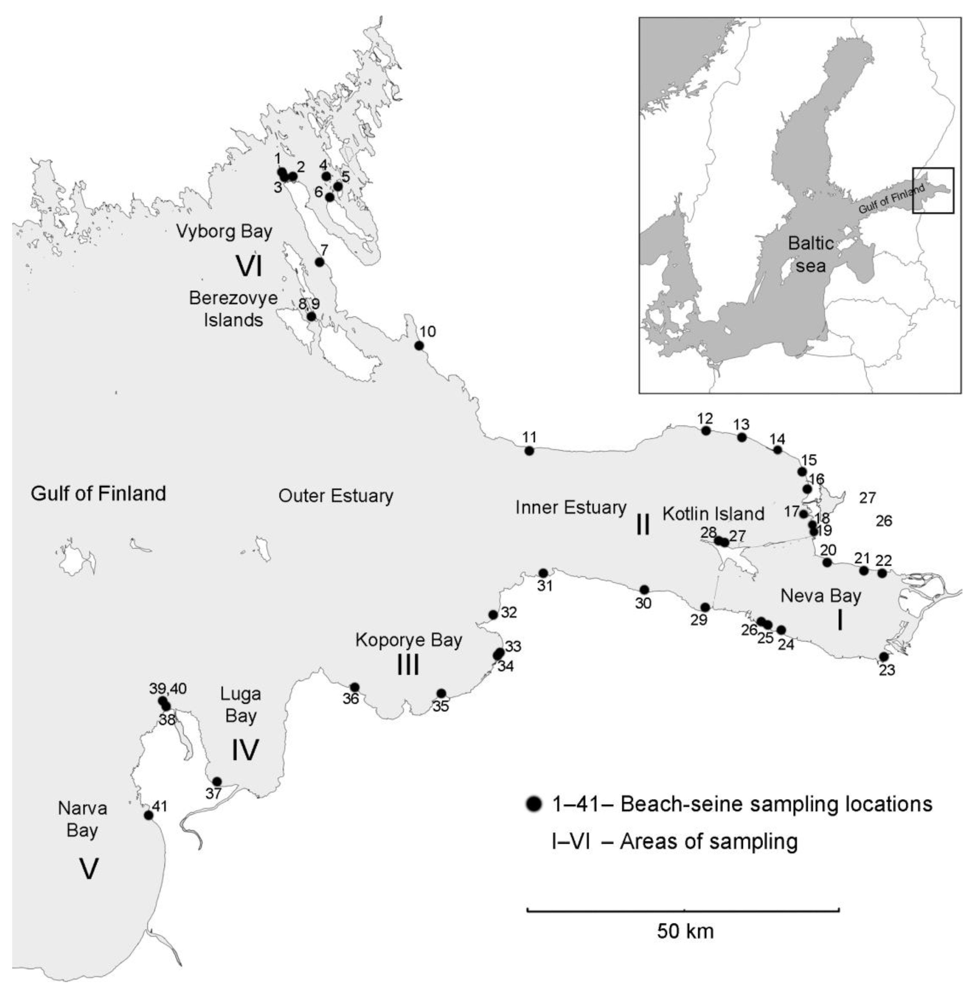
2.1. Study Site, Sampling and Laboratory Analysis

The investigation of coastal fish community of the eGoF was conducted during 2011–2017. In total, 41 locations (Figure 1) were sampled at depths of up to 1.2 m; 151 beach-seine catches were collected. Fishes were caught in the Neva Bay (loc. 20–26), Inner Estuary area (loc. 11–19 and 27–31), Luga Bay (loc. 37), Koporye Bay (loc. 32–36), Narva Bay (loc. 38–41), Vyborg Bay, and the northern coast of the Outer Estuary (loc. 1–10).
The sampling was performed during ice-free season from May to November. All samples were sorted to spring (till June 15), summer (from 15 June to the 15 September), and autumn (from 15 September) periods. Sampling periods were not equal to calendar seasons due to sampling often occurring in alternating months. For example, samples made in late August and early September in the same temperature and weather conditions were combined.
The fishes were captured with a hand-towed beach-seine (length 10 m, wings 1.5 m high, the bag 3 m in length, a mesh-size 10 mm in the wings, and 0.5–4 mm in the cod end). Caught fish were anesthetized with clove oil and then preserved with 4% formaldehyde.
Investigation of samples and taxonomical determination of fish specimens were conducted in the laboratory. Life stages of fish specimens (adult, juvenile) were estimated by the means of standard length (SL, mm). Ecological guilds (freshwater, marine, anadromous, estuarine fish species, etc.) are given in accordance with Thiel et al. [22,23]. Species composition, species richness, occurrence (V), and density (D) of different species were estimated for each catch.
Species richness was equal to the number of fish species in the sample.
Frequency of occurrence (V; %) was estimated according to:
V = 100   ×   A a
where A is a total number of samples and a is a number of samples where certain species was caught. The species was identified as a “core” fish species by means of V ≥ 50%; such species most frequently occurred in the samples. A species was considered as “secondary” if it was recorded in 25–49% of samples, “rare” if the V was from 8 to 24%, and “sporadic” for V ≤ 7% [24].
Density (D; ind./100 m2) was estimated as number of fish individuals (Ni; ind.) per 100 m2 of the sampled area (Ssmpl; m2) [25]:
D = 100   ×   Ni S smpl
where, Ssmpl was estimated as hauling distance (25–90 m) multiplied by mouth width of the beach seine while sampling (around 6 m). Hauling distances were measured using optical laser distance meter Sturman LRF 400 with the accuracy of 1 m at the start of each hauling.

2.2. Measurement of Environmental Parameters

Environmental variables were measured each time and in each location where fishing was conducted. Water salinity and temperature were measured with Hanna HI98130 Combo tester (see Table A1). Turbidity, bottom substrates composition, and vegetation abundance were estimated as ranked parameters and overviewed below (Table 1). Ranks or indices are commonly used to describe habitat heterogeneity in ecosystem studies [11]. Salinity was estimated both in absolute values and ranked for the aim of the analysis, which demands the ranked data. Ranking was based on classification of water masses and salinity “barriers” [26,27,28]. In case of turbidity estimation at the shallows, Secchi disk was useless due to transparency was commonly more than depths on the sampling site.

2.3. Statistical Analysis

Statistical analyses were based on the density data (D) of the fish species in samples. To avoid the overwhelming influence of high abundance species, the raw data were transformed using fourth root transformation. The site/species matrix, where each site has the set of environmental and seasonal variables, was analyzed using canonical correspondence analysis (CCA). CCA is a weighted-averaging method for directly relating community data (abundance of species) with environmental and seasonal conditions by constraining the species ordination to a pattern that correlates maximally with designated variables. The analysis was carried out using an algorithm of Legendre and Legendre [29] implemented in Past 4.03 [30].
Statistical significance in the abundance and occurrence of fish species between groups of sampling locations, classified on the basis of seasonal factors and environmental variables (see Table 1), were estimated using ANOSIM [31]. The analysis was calculated based on Bray–Curtis distance. The sequential Bonferroni correction was applied for significance estimation. ANOSIM was performed using Past 4.03.
Discriminant Function Analysis (DFA) of abundance data was performed using STATISTICA 10.0.1011 (StatSoft, Tulsa, OK, USA) to estimate the degree of differentiation between the groups of sampling sites. The quality of discrimination was assessed based on the Wilks’ Lambda and F-test statistics. Wilks’ Lambda values close to 0 indicate strong discrimination. The result of this analysis is visualized using a scatterplot of canonical values in the space of the first and second discriminant axes.
The SIMPER procedure was used to identify the species that contributed the most to the pattern of similarities (in PRIMER v.6) and differences (in Past 4.03) between samples. For each group of samples, differentiating (with the greatest contribution to the matrix of differences between the groups of samples) and characterizing (with the greatest contribution to the matrix of similarity between samples within one group) taxa were identified [32,33].
Pairwise correlation between environmental variables was assessed using Spearman’s coefficient since a normal distribution has not been proven for these parameters. Differences between the values of factors for different areas and seasons were assessed using the Kruskal–Wallis test (in Past 4.03). The same test was used for cross-site comparisons of total density of fish and species richness. The Kruskal–Wallis test was also used to identify differences in the densities of individual species under different environmental factors. Species richness was calculated in Past 4.03.

3. Results

3.1. Results of Field Observations

3.1.1. Coastal Fish Species Diversity

According to the result of beach-seine sampling in 2011–2017, the fish community of the coastal shallow waters of the eGoF includes 34 species of 13 families (Table 2). The cyprinids (Cyprinidae) were dominant by species number (15 species or 44%). The majority of the fish species caught in shallows were freshwater species (68% of all species). Most of the fish specimens in the shallow water catches were juveniles. Adults were abundant for resident coastal species such as Gobio gobio (Linnaeus, 1758); Alburnus alburnus (Linnaeus, 1758); Cobitis taenia Linnaeus, 1758; Phoxinus phoxinus (Linnaeus, 1758); Perccottus glenii Dybowski, 1877; Gasterosteus aculeatus Linnaeus, 1758; Pungitius pungitius (Linnaeus, 1758); Pomatoschistus microps (Kroyer, 1838); and Proterorhinus marmoratus (Pallas, 1814) (Table 2). Adult, though generally not large, individuals were also recorded among some species such as R. rutilus, P. fluviatilis; G. cernua; Gobio gobio (Linnaeus 1758); Scardinius erythrophthalmus (Linnaeus, 1758); Leuciscus leuciscus (Linnaeus, 1758); and Neogobius melanostomus (Pallas, 1814).
According to the frequency of occurrence, five species (A. alburnus, R. rutilus, P. fluviatilis, G. gobio, and G. cernua) constitute the “core” of the coastal fish assemblage in the eGoF. Notably, 17 species (50% of species list) occurred sporadically (Table 2). Nerophis ophidian (Linnaeus, 1758); Barbatula barbatula (Linnaeus, 1758); and Pelecus cultratus (Linnaeus, 1758) were all recorded on single occasions.
Alburnus alburnus had the highest mean density (mean ± SE = 60.0 ± 16.5) in the area studied. R. rutilus and P. fluviatilis, which had the second highest D-values, had only a third of the density of Alburnus alburnus (Table 2). Pomatoschistus microps (Kroyer, 1838) had the highest mean density (mean ± SE = 59.2 ± 22.4) among “secondary” species; mean D-value for this goby species was the second highest among all species in the list. “Rare” and “sporadic” species were generally not abundant (except for alien P. glenii).

3.1.2. Environmental Conditions

According to the results of the environmental parameters measured during the fish sampling, the coastal habitats of the eGoF are very diverse and differ in the bottom substrate, the presence and type of vegetation, and in the main hydrological parameters—salinity and turbidity (Table A1).
Spring, summer, and autumn temperatures in the coastal shallows were significantly divergent (Kruskal–Wallis, H = 49.5; p < 0.001). Still, the water temperature during the summertime was not significantly different between coastal areas (Kruskal–Wallis, H = 9.1; p = 0.104); therefore, this factor could not have a major effect on the difference in fish communities between them.
The salinity gradient observed in shallow waters varied between 0.05–4.50‰. The fresh waters (salinity < 0.5‰) were registered in the Neva Bay. The most saline areas (salinity ≥ 3.0‰) were in the Narva and Luga Bays (Table A1). The highest fluctuations in water salinity were recorded in the Inner Estuary along the southern coast (loc. 29–31), where both the Neva River runoff and the saline water inflows from the open part of the Gulf are present.
Shallow water habitats of the eGoF are represented by the solid sand beaches (32% of locations; 40% of samples), stony bottom (17% of locations; 12% of samples), and mostly by mixed sandy–stony bottoms (stone fraction varied from small pebbles to boulders) with a various presence of silts and clays (41% of locations; 48% of samples). Interannual changes in the type of bottom substrate were noted at four locations (loc. 13; 15; 30; 31), which could be due to the storms and erosion processes in the coastal areas that cause washing or mudding of bottom sediments. The greatest amount of pure stony substrates in the shallows was found along the northern coast from the Inner Estuary to the Vyborg Bay; pure sandy bottom—along the southern coasts of the Neva Bay and Inner Estuary. Boulders are common westward from the Inner Estuary.
The degree of overgrowth of coastal areas varies quite strongly; beaches devoid of any vegetation often border on dense reedbeds (for example, near locations 18; 21; 25; 29; 35). The investigated coastal areas where macrophytes were completely absent during the whole season accounted for 29% of all locations sampled (Table A1). At the locations where submerged macrophytes were presented in summer (loc. 13; 20; 22), they were often completely absent in spring and autumn.
The overgrowth of filamentous algae in the coastal locations was most often observed in the Koporye and Narva Bays (50% of locations; Table A1). In the Neva Bay and Inner Estuary, filamentous algae were abundant just at 2% and 6% of locations, respectively. At the same time, filamentous algae mats tossed ashore by the waves were often observed along the coastline, especially outside the Neva Bay.
High turbidity of water was most often observed in the Neva Bay and Inner Estuary; clear water—in the Vyborg and Narva Bays. In the westward areas turbidity was lower and associated with the resuspension of fine sediments after storms.
Correlation was found for certain parameters: salinity—turbidity (R = −0.38, p < 0.001), salinity—presence of filamentous algae (R = 0.31, p < 0.001), temperature—presence of filamentous algae (R = 0.43, p < 0.001).

3.2. Results of Data Analysis

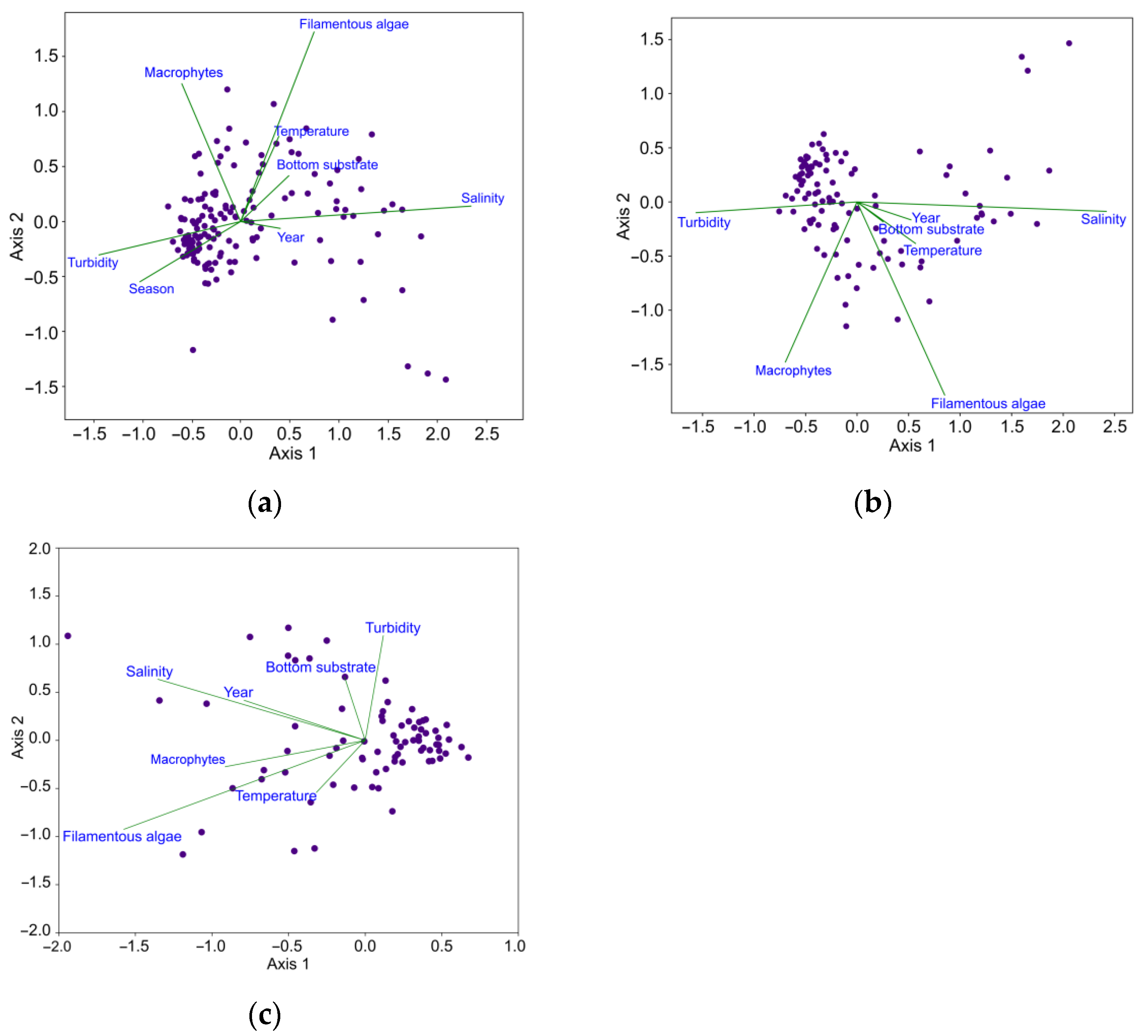
3.2.1. Identification of Major Environmental Factors Affecting the Fish Community

Two variables related to the period of sampling (‘Year’ and ‘Season’), four abiotic (‘Bottom substrate’, ‘Turbidity’, ‘Salinity’, ‘Temperature’), and two biotic (‘Macrophytes’ and ‘Filamentous algae’) environmental factors were analyzed with CCA (Figure 2).
The influence of the sampling season on the fish assemblage is rather high. According to the results of CCA, the length of the ‘Season’ vector was approximately equal to half the length of the highly contributing ‘Salinity’ vector (Figure 2a). Therefore, for the subsequent analysis of the association of environmental factors and the fish community (ANOSIM, DFA) only samples of summer period (as the most numerous) were selected. Differences related to the year of sampling are rather low (length of “Year” vector was equal to 17% of the length of ‘Salinity’ vector) (Figure 2a). The effect of water temperature was low for all three seasons (spring, summer, and autumn) as well as for the summer months. The length of the “Temperature” vector was less than 40% of the longest vector’s length (Figure 2a,b).
In the summer period, four environmental variables (‘Salinity’, ‘Turbidity’, ‘Macrophytes’, and ‘Filamentous algae’) had a high influence on the fish species composition and their abundance (Figure 2b). According to the results of ANOSIM, both ‘Salinity’ (used here as ‘Salinity ranges’) (ANOSIM, R = 0.476; p = 0.0001) and ‘Filamentous algae’ (ANOSIM, R = 0.153; p = 0.0001) provided the most differences between sample groups. Such parameters, as ‘Turbidity’ (ANOSIM, R = 0.101; p = 0.0001) and ‘Macrophytes’ (ANOSIM, R = 0.077; p = 0.001) also remarkably contributed. Due to the significant impact of salinity on the fish species composition and density, we have selected samples within salinity up to 1.9‰ (70% of all summer samples; that were enough for the analysis) for the second round of analysis to minimize dominative effect of ‘Salinity’ factor (Figure 2c). However, the influence of salinity was still significant within gradient 0.0–1.9‰ (ANOSIM, R = 0.305; p = 0.0003). The second most substantial factor was ‘Filamentous algae’ (ANOSIM, R = 0.124; p = 0.002), followed by ‘Macrophytes’ (ANOSIM, R = 0.071; p = 0.006). The effect of ‘Turbidity’ within salinity up to 1.9‰ was lowered, being near significant (ANOSIM, R = 0.055; p = 0.057). All other examined variables did not demonstrate significant differences between sample groups.
The locations grouped by the ‘Salinity ranges’ were significantly different according to the data on the fish species composition and density (DFA, Wilks’ Lambda = 0.0959, approx. F = 3.6191, p < 0.0001), with the exception for ‘ranges’ 0 and 1 (p0–1 = 0.2672) (Figure 3a). Thus, the fish communities of locations within salinity ranging from 0.0 to 1.9‰ can be considered homogeneous. Therefore, two groups of samples composing ‘Salinity ranges’ 0 and 1 (see Table 1) were combined for the reasons of subsequent examination. Since the effect of salinity on the fish community was to be highest, the subsequent analysis of the remaining factors (‘Filamentous algae’, ‘Macrophytes’, and ‘Turbidity’) was conducted on samples within the salinity range 0.0–1.9‰ to exclude the effect of the salinity gradient on the fish distribution. Geographically, the samples collected within this salinity (ca. 70% of total samples) belong to the Neva Bay (all samples < 0.5‰) and the Inner Estuary (just samples in 0.0–1.9‰).
Significant differences between all groups of samples within salinity 0.0–1.9‰ were obtained for ‘Filamentous algae’ (DFA, Wilks’ Lambda = 0.1872, approx. F = 3.1576, p < 0.0001) (Figure 3b). For the ‘Macrophytes’ (Figure 3c), a significant level of differences was also detected (DFA, Wilks’ Lambda = 0.3152, approx. F = 1.8818, p = 0.0045); there was no difference only between the group of samples without any macrophytes and the samples where only submerged vegetation was present (p0–1 = 0.1912).
DFA revealed the significant level of differences for ‘Turbidity (Figure 3d) (Wilks’ Lambda = 0.3884, approx. F = 1.8618, p = 0.0021). However, only the groups of samples taken at the most turbid and the clearest water were significantly different during the summer period (p0–2 < 0.0001). The differences only between the extreme groups can be explained by ranking without direct measurements of the turbidity, when the probability of estimation’s error may be rather high. This, along with the results of ANOSIM, suggests rejecting the ‘Turbidity’ factor in the downstream analysis.

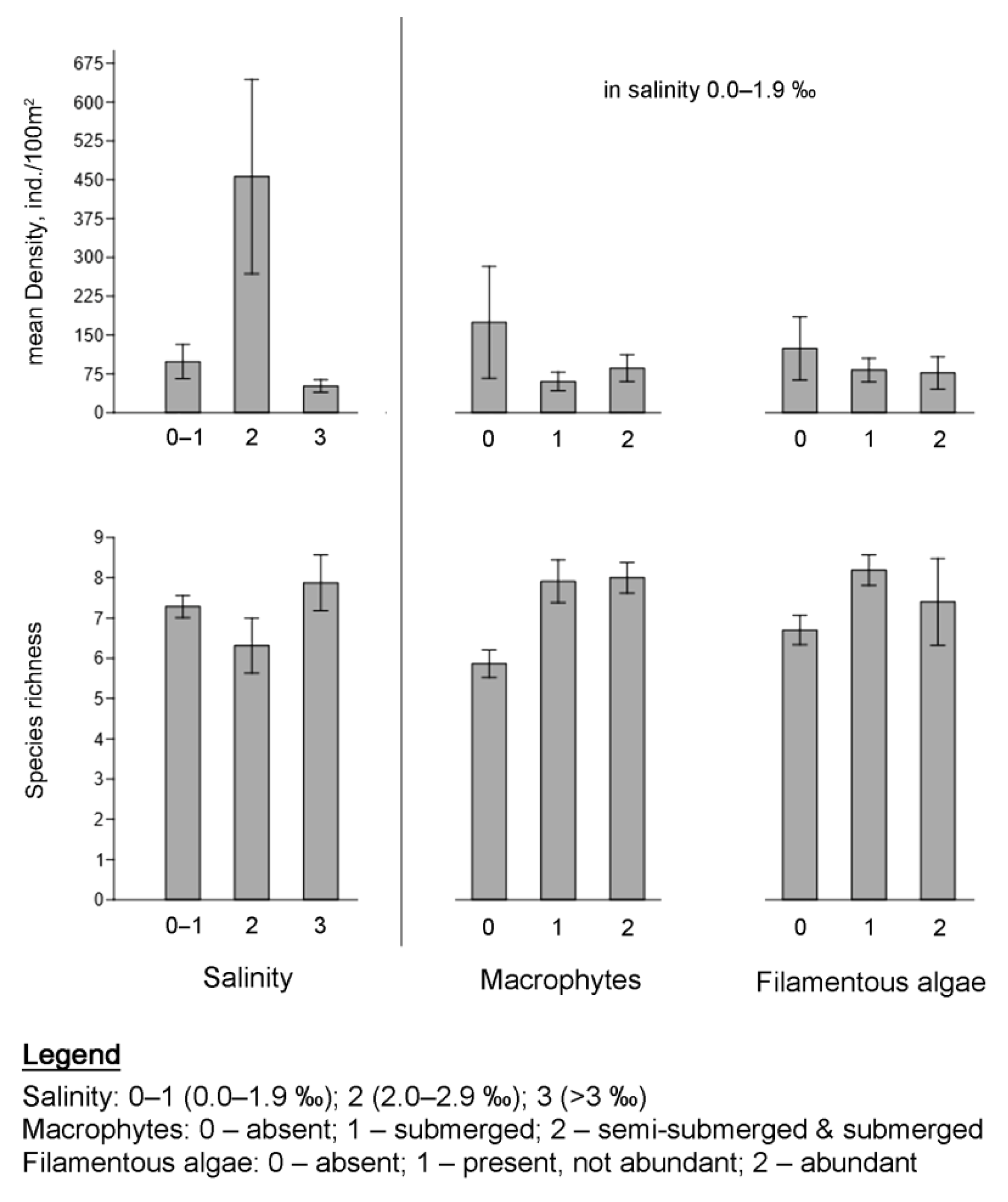
3.2.2. Influence of Environmental Factors on the Species Richness and the Fish Density

A moderate positive correlation of the fish density both with water temperature (R = 0.31, p < 0.001) and ‘Filamentous algae’ (R = 0.38, p < 0.001) was detected. The same was found between species richness and ‘Macrophytes’ (R = 0.37, p < 0.001).
The fish density was at maximum (Kruskal–Wallis, H = 7.8; p = 0.02) with the salinity range 2.0–2.9‰ (Figure 4). No significant differences in the fish density were observed for other factors. The species richness did not differ significantly between different salinities. This index was lower both within the zero values of ‘Macrophytes’ (Kruskal–Wallis, H = 13.2; p = 0.001) and ‘Filamentous algae’ (Kruskal–Wallis, H = 7.8; p = 0.02).

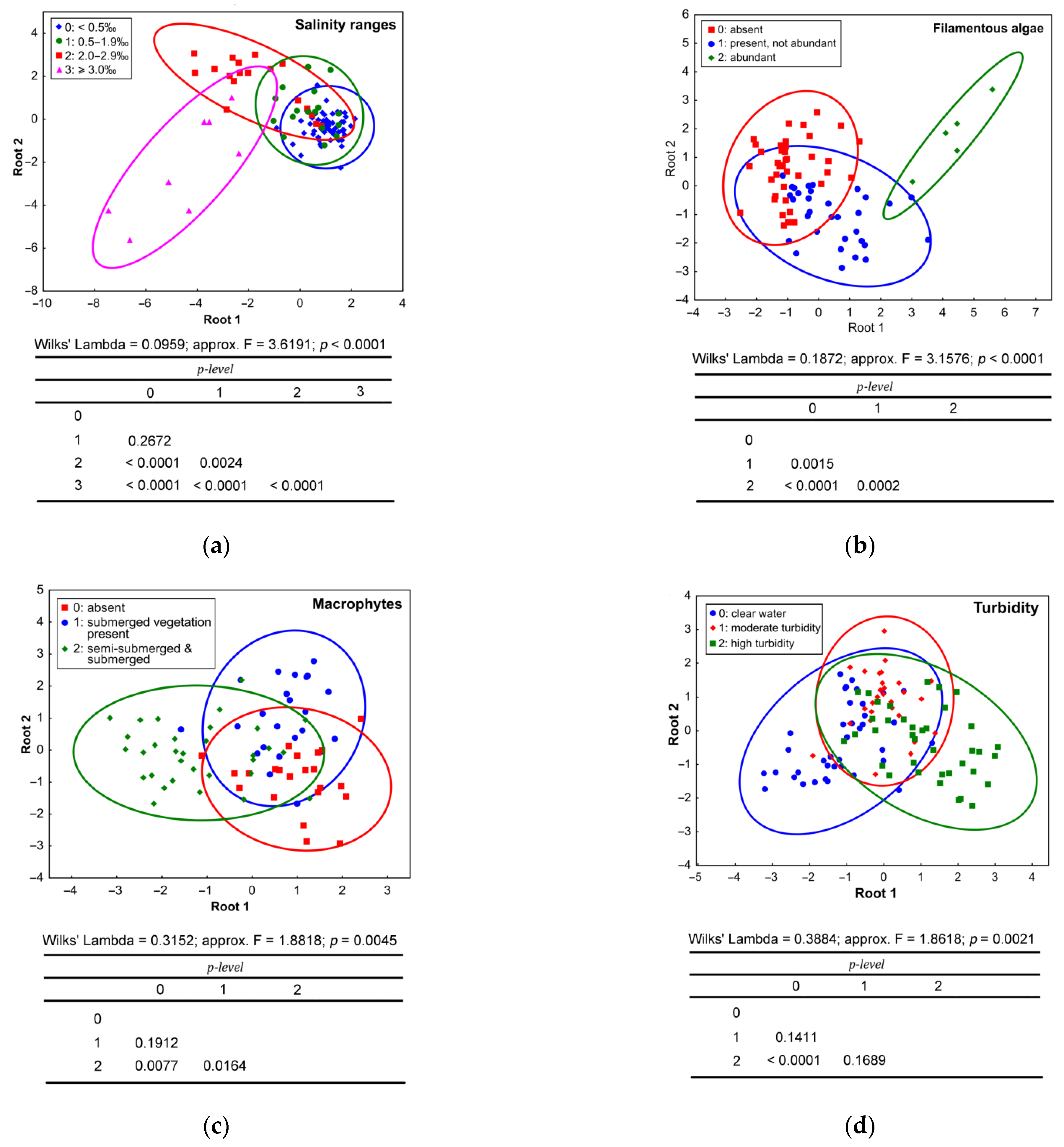
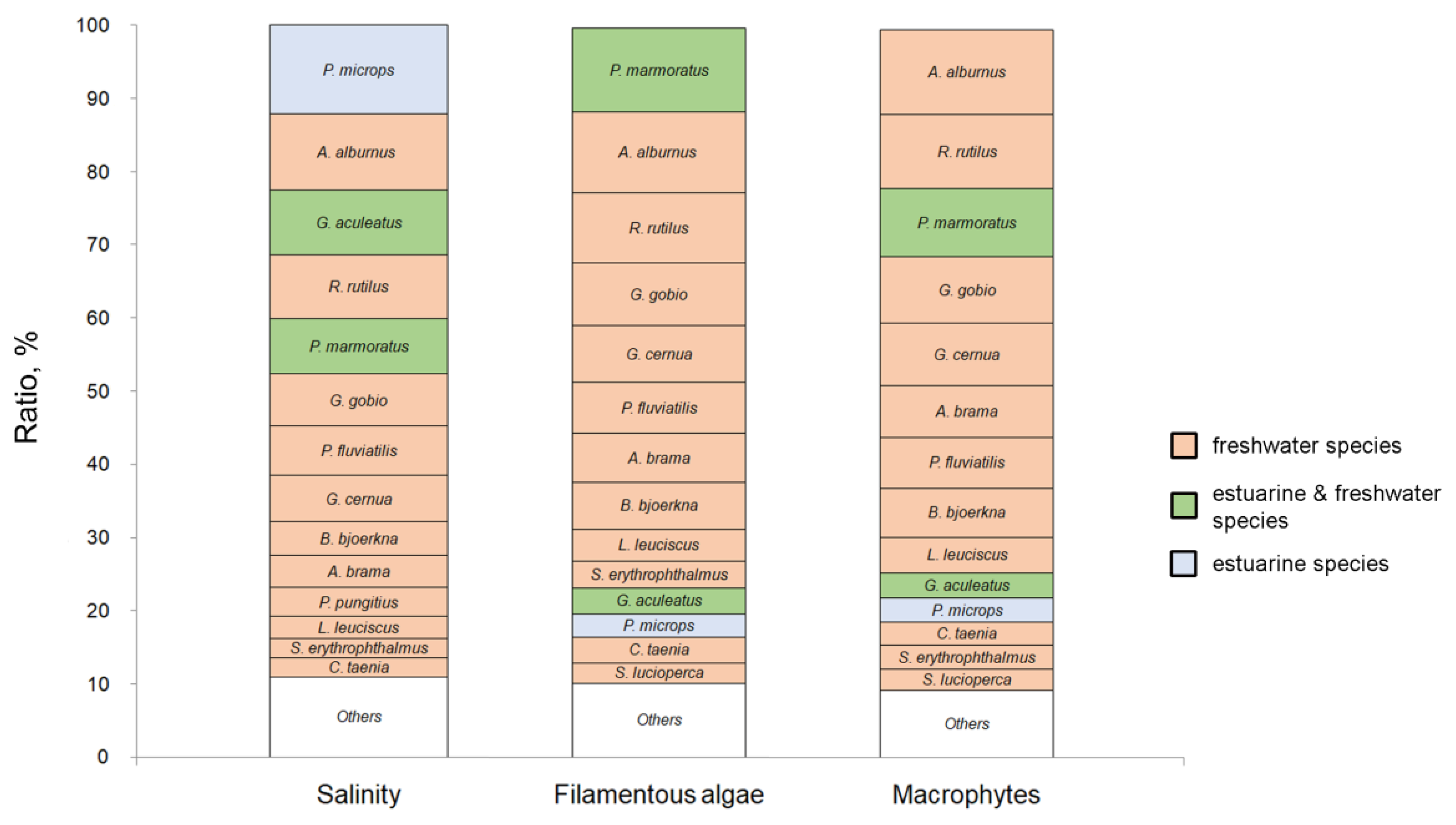
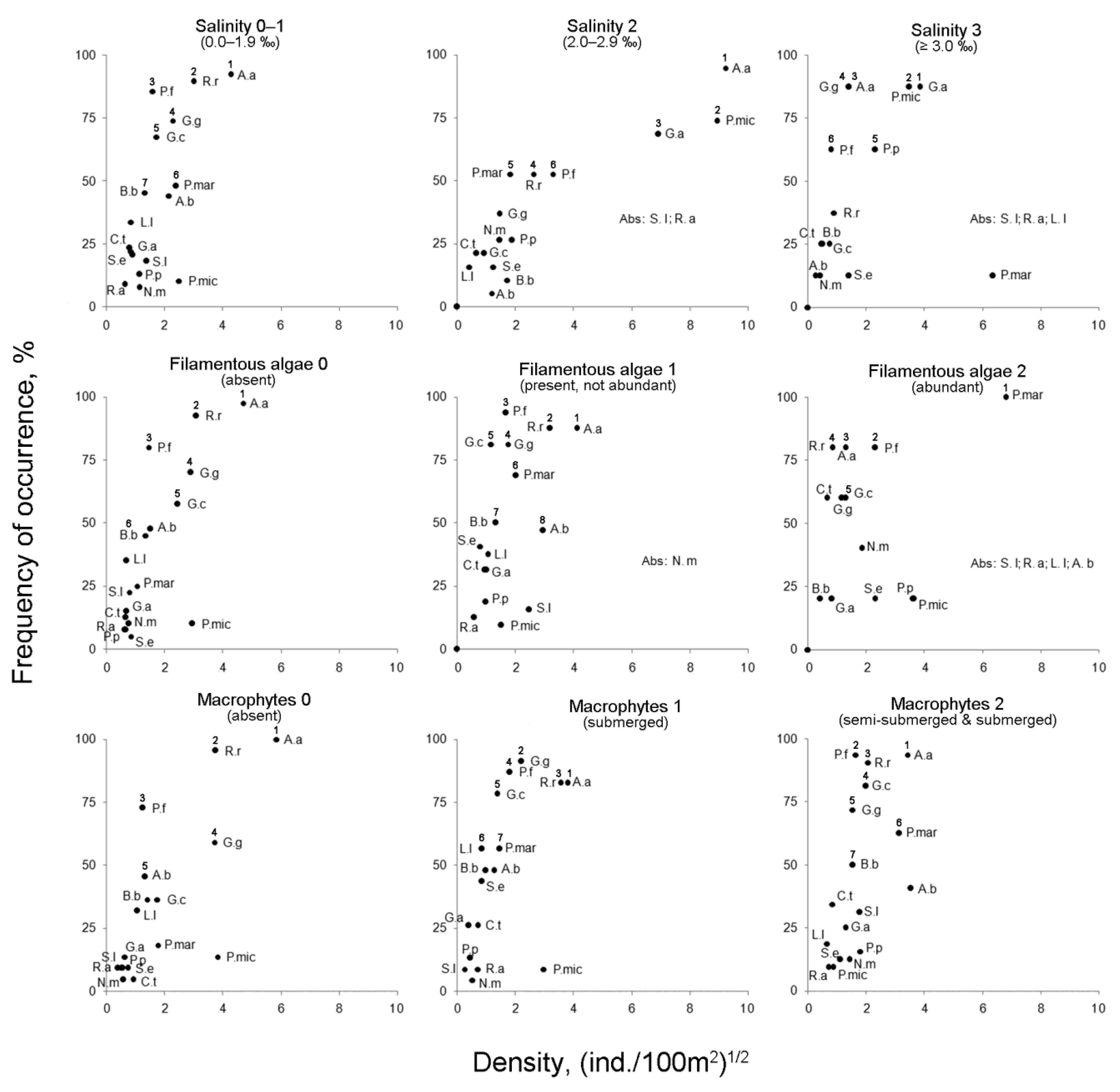
3.2.3. Differences in the Species Composition, Occurrence, and Density

Differences in the species composition, occurrence, and density of certain fish species between groups of samples influenced by environmental factors were studied on the material collected during summer.
Discriminating taxa by the results of SIMPER are shown in Figure 5. Around 90% of dissimilarity between groups of samples (0; 1; 2; etc. see Materials and Methods) within each environmental factor was associated with 14 species (41% of species list; see Table 2). The first five discriminating taxa always included P. marmoratus, A. alburnus, and R. rutilus. In the case of ‘Macrophytes’ and ‘Filamentous algae’, around 50% of dissimilarity for each environmental factor was provided by four “core” freshwater species and P. marmoratus. ‘Salinity ranges’ were differed by two “core” freshwater and three “secondary” estuarine species. “Rare” and “sporadic” species together provided less than 20% of dissimilarity.
The species typifying each group of factors were also usually composed of the “core” species and some mostly occurring and abundant “secondary” species (see numbers on Figure 6). The number of such species by the results of SIMPER varied from five to eight. Alburnus alburnus, R. rutilus, and P. fluviatilis were always among the list of typifying taxa. Pamatoshistys microps and both species of sticklebacks were typical for high salinities, while P. marmoratus was typical for the presence of filamentous algae and macrophytes.
Nonetheless, the frequency of occurrence and mean D of certain species remarkably varied for each variation of environmental factors. Variability of the V and D values for 17 fish species (sporadic species were not overviewed) within different environmental variables is given in Figure 6. Most of these species occurred in the locations with any values of ‘Salinity ranges’, ‘Macrophytes’, and ‘Filamentous algae’ (except for S. lucioperca, R. albipinnatus, N. melanostomus, A. brama, and L. leuciscus). The frequency of occurrence achieved > 50% for A. alburnus and P. fluviatilis in all categories of studied variables. The highest average D values were demonstrated mainly by “core” (in the case of whole eGoF; see Table 2) and “secondary” species.
The species composition with V > 50% changed along the salinity gradient (although the gradient seems to be relatively small, 0.0–4.5‰). Pomatoschistus microps, G. aculeatus, and P. pungitius replaced G. cernua and R. rutilus as the most frequent species with a salinity increase (Figure 6). The frequency of occurrence of the P. marmoratus was > 50% at a salinity > 2‰, but at a salinity ≥ 3‰ its V-value significantly decreased (12.5%). Inversely, the V-value of G. gobio decreased in the salinity 0.5–1.9‰. Romanogobio albipinnatus, S. lucioperca, and L. leuciscus were not recorded at a salinity ≥ 3‰. The average D-values were the highest for the most of species at a salinity of 2.0–2.9‰, while the same for a P. marmoratus and P. pungitius was revealed at ≥ 3‰.
With an increase of filamentous algae abundance, V-values of the P. marmoratus and C. taenia heightened significantly (from 25 to 100% and from 12 to 60%, correspondingly). C. taenia is the only one “rare in the eGoF” species with such high occurrence variation. Maximal abundance of filamentous algae coincided with remarkably decreased V-values of B. bjoerkna and S. erythrophthalmus, while four species (R. albipinnatus, A. brama, S. lucioperca, and L. leuciscus) fully disappeared. Mean D-values of the P. marmoratus (Kruskal–Wallis, H = 9.8; p = 0.007) increased most significantly at the highest abundance of filamentous algae.
Only four species demonstrated V-values ≥ 50%, when macrophytes were absent. With the emergence of submerged macrophytes, the V-values of P. marmoratus, L. leuciscus and C. taenia notably increased (from 18 to 57%; from 19 to 57%; and from 4 to 26%, correspondingly). In semi-submerged macrophytes, the V-values of P. marmoratus and C. taenia continued to increase; additionally, B. bjoerkna occurred with a frequency of 50%. The average D-values of A. alburnus were the highest where macrophytes were absent; with the appearance of semi-submerged vegetation, A. brama became the most abundant (Figure 6).

4. Discussion

Our study revealed that 34 fish species recorded in the shallows of the eGoF select favorable habitats among the heterogeneous coastal biotopes, which are highly diverse in the studied area [10]. We have identified three key environmental parameters that most affect the distribution of the species composition and density—(i) water salinity, (ii) the presence of macrophytes, and (iii) the presence of filamentous algae. They were also recognized as the most impactful to the distribution of aquatic organisms in other areas [7,11,34]. These key environmental parameters caused the changes in species richness, composition of typical taxa, variations in the occurrence, and density. We suggest that our results are essential for future ecological investigations, coastal ecosystem management, and conservation of the Baltic Sea ecosystem. It provides opportunities for modelling potential fish assemblages based on environmental data, which is the aim of the future research. Below, we consider the impact of certain parameters in more detail.

4.1. Salinity

Water salinity was the most significant factor affecting the composition and distribution of the fish in the eGoF. This is in good agreement with the common ideas about the formation of biocenoses [35]. Thorman [11] has stated that salinity was the most impactful factor in the northern Baltic Sea, affecting a number of species. The eGoF is an extended estuary with a distance from the mouth of the Neva River to Gogland Island ca. 180 km. It has a bright pattern of westward salinity gradient from near-zero values to 5‰ [36]. Periodical variations in salinity, which are typical in the eGoF [37], were also detected in the coastal zone during our research. They are associated with the predominance of the inflow of brackish waters from the west or the runoff of fresh water from the Neva River in the east [37]. In the western part of the Gulf of Finland (west of Gogland Island), the salinity gradient is less pronounced (salinity 4–6‰) [38].
The fish species composition in the eGoF with the freshwater species prevailing is different to that from the western part of the Gulf [39,40]. The core of the fish assemblage of the eGoF coastal area was represented by five freshwater species—A. alburnus, R. rutilus, G. gobio, P. fluviatilis, and G. cernua. According to other recent studies, these species were also common in estuaries and coastal areas in different parts of the Baltic Sea [4,12,16,39]. Generally, the “core” of fish assemblage is composed of species that are adapted to various types of habitat, from small freshwater ponds to large brackish water areas such as the Baltic Sea coastal zone [12]. The same freshwater species (R. rutilus, P. fluviatilis, and G. cernua) were the most abundant and distributed in the closest Finnish coast of the Gulf of Finland [12]. The common bleak Alburnus alburnus is a relatively rare species beyond the eastern Gulf of Finland and inhabits similar estuarine areas [4,41]. Generally, A. alburnus was not as numerous as R. rutilus and P. fluviatilis, which are more common and widely distributed in the Baltic Sea.
Beyond the oligohaline Gulf of Finland, the occurrence of freshwater fishes declines notably. At the shallow habitats of the more saline waters of the Baltic Sea, marine and brackish fish species predominate—A. tobianus, Hyperoplus lanceolatus (Le Sauvage, 1824); Platichthys flesus (Linnaeus, 1758); Scophthalmus maximus (Linnaeus, 1758); C. harengus membras; S. sprattus balticus; and P. minutus [3,4,5,12,16]. According to our results, no significant change in the fish species composition was revealed in the coastal shallows of the eGoF within a salinity gradient of 0.0–4.5‰. However, with an increase of water salinity, the occurrence and number of estuarine species (e.g., P. microps and G. aculeatus) was more frequent. At the highest measured salinity (3.0–4.5‰), only a few freshwater “secondary” and “rare” species were absent (S. lucioperca, R. albipinnatus, and L. leuciscus). In total, only four marine species were observed in the eGoF shallows; all of them were “sporadic”.
According to classifications of water masses [26,27], the coastal waters of the eGoF are classified as freshwater (up to 0.5‰) and oligohaline (from 0.5 to 5‰). Additionally, Aladin and Plotnikov [28] determined that waters with a salinity up to 2‰ to be the “main freshwater zone”, and from 2 to 5‰ to be the “transitional zone” from fresh to brackish waters. This is below the level of the “critical salinity” barrier or “α-horogalinikum” (5–8‰) evidenced by Remane [42] and Khlebovich [26,43]. “Critical salinity” is the nucleus of brackish waters and is characterized by a notable decrease in the number of both freshwater and marine species changed by “brackish water” fauna [28]. Nevertheless, inside oligohaline waters, it is assumed that there is an intermediate oligohaline barrier or “δ-horogalinicum” (0.5–2.0‰) separating fresh and brackish waters [28]; this barrier restricts the spreading of “true freshwater” stenohaline species to brackish waters [27,28]. Our results showed that the fish community within water a salinity < 2.0‰ (fresh and “δ-horogalinicum” waters, or “main freshwater zone”) was homogeneous, and at the same time it differed by species composition and individual occurrences from those within a salinity ≥ 2‰ and ≥ 3‰. Moreover, the last two groups were also significantly different. This suggests that the “δ-horogalinicum” also exists for the fish community. Estuarine and marine species were lacking within a salinity < 2.0‰. Only P. microps, P. marmoratus, N. melanostomus, and G. aquleatus (the last three are mostly euryhaline) were recorded. Based on this observation, the coastal fish community in the inner parts of the eGoF (Neva Bay and part of the Inner Estuary) can be classified as typical freshwater fauna of rivers and lakes. While the outer parts (Vyborg, Koporskaya, Luga, and Narva Bays) are more complex and composed of freshwater and estuarine–brackish water fauna with the inclusion of some marine species. The combination and temporal exchange of these groups occurs in the Inner Estuary (most pronounced along the southern coast), due to the intensive mixing of water masses—Neva River runoff from the east and brackish water inflows from the west.

4.2. Filamentous Algae

Filamentous algae are the second key factor affecting the coastal fish community. A relatively low biomass of filamentous algae provides a complex habitat rich in resources for the benthic fauna and refuges for small fish, crustaceans, and gastropods [44,45]. At the same time, the accumulation of large mats of destructive filamentous algae along the coast in late summer is accompanied by an intense eutrophication and a drop in the dissolved oxygen concentration [46,47], which has a detrimental effect on the coastal benthic community [48]. The increase in the biomass of filamentous algae in the Baltic Sea caused significant changes in the fish community and a decrease of fish abundance in shallow waters as shown by Pihl et al. [34]. In addition, filamentous algae may produce toxic exudates resulted in the increased mortality of fish eggs [49,50]. Cladophora glomerata (L.) Kütz, Ulva intestinalis L., and Pylaella littoralis (L.) dominate in the community of filamentous algae in various areas of the eGoF [51]. The development of C. glomerata in the eGoF is the most intensive in comparison with other areas of the Baltic Sea [47,52]. Algal mats support the complex and highly productive invertebrate communities of the littoral zone in the Neva Estuary that feed on it [48,53]. At the same time, Demchuk et al. [54] show that such invertebrates (chironomids, zooplankton, and insects) that occurred in algal mats were important food components for mass fish species inhabiting coastal zone of the Gulf of Finland.
Our results show that although the species richness was minimal at the complete absence of filamentous algae, the greatest variation of species richness was observed at a high abundance of filamentous algae (Figure 4). The list of fish species was decreased by four species (S. lucioperca, R. albipinnatus, L. leuciscus, and A. brama) at a high abundance of filamentous algae. This was the shortest species list when compared with the samples for other environmental variables (Figure 5). At the same time, a moderate positive correlation was detected between the abundance of filamentous algae and the density of fish in catches. Moreover, the density and the occurrence of the alien species, tubenose goby P. marmoratus, increased significantly with an increase in filamentous algae biomass; this species prefers such a habitat [55]. Thus, the influence of filamentous algae on the species richness and density of the coastal fish assemblages in the eGoF seems to be ambivalent.
Apparently, filamentous algae have the greatest negative effect on the reproduction of fishes—on the eggs and larvae, particularly; this effect is more pronounced during algae dieback [45,56,57]. Despite this, the postlarvae and early juveniles of gobies, cyprinids, and sticklebacks were found in mass in habitats with abundant growths of filamentous algae as well as among their detached fragments in the water column. This is probably due to the juveniles being attracted by invertebrates developing on algae mats. Juveniles, compared to eggs and larvae, are able to actively migrate in shallow waters and avoid anoxic zones in algal mats. Nevertheless, notable changes in the fish assemblage under the pressure of a continuous increase of filamentous algae in the Baltic Sea can be expressed in a long-term period by the disruption of fish reproduction [58].

4.3. Macrophytes

Macrophytes significantly influence the structure of the fish community [34]. The aquatic vegetation is important for the successful reproduction of many fish species in the Baltic Sea, providing spawning substrate, nursery grounds, and shelter from predation for juveniles [4]. The abundant vegetation positively correlated with the species richness and abundance of fish that find refuge and food among the plants [59,60].
Overgrowing by semi-submerged macrophytes (Phragmites spp., Scirpus spp., Typha spp., etc.) has been occurring continuously in the eGoF coastal areas in recent decades [61,62]. The most intense expansion of reeds is most common in the Neva Bay and the Inner Estuary. This process was enhanced after the Saint Petersburg Flood Prevention Facility Complex (SPb FPFC) dam construction [63]. At the same time, communities of submerged macrophytes (Potamogethon spp., Elodea sp., Stratiotes sp., etc.) are extremely unstable here due to the intense impact of hydrotechnical works and increased water turbidity [62,64].
Our study showed that the presence of macrophytes in the eGoF coastal shallows had a positive effect on the fish species richness (see Figure 4). Remarkably, the fish community of thickets of semi-submerged macrophytes significantly differed from that of thickets of submerged macrophytes and shallows with no vegetation in terms of the composition and abundance of certain fish species (see Figure 3). At the same time, the absence of such differences between the last two groups (‘submerged’ and ’no vegetation’) might be explained by the impossibility of soft submerged vegetation to reduce a wind-wave impact, as compared to semi-submerged thickets. In southwest Finland, dense reed belts are spawning and nursery areas for ten (undoubtedly, even more) fish species [4]; 9/10 of which were recorded in our study. Apparently, the macrophytes make habitat more complex and more suitable for the concentration of larvae and mature and spawning individuals in different seasons. Studying the fish assemblages in thickets of different types, their relationship at different life stages is the aim for further research. Based on the current trend of the expansion of vegetation in eGoF shallows, we suggest further changes in the fish community.

4.4. Other Environmental Factors

Water turbidity can have a variety of effects on fish depending on the intensity and origin. Its effect can be both negative (depression of respiration and metabolism, changes in feeding behavior, disturbed migration and distribution, silting the eggs and larvae, etc.) and positive—through a change in the prey–predator relationship and attractivity for some actively moving fish [65,66,67]. In recent decades, a periodic increase in water turbidity in the eGoF associated with dredging or blooming has been observed. The turbidity is especially high in the Neva Bay [68]. Eutrophication resulting in summer water blooms can significantly impact fish communities over a large area [69]. At the same time, Korpinen et al. [70] showed that nutrient inputs (which provide the eutrophication increase) were estimated as one of the highest pressures in the entire Baltic Sea area. In addition, increased turbidity occurs after storms and water level fluctuations in shallow waters [65]. Although we observed the differences between fish communities inhabiting highly turbid and clean water, we were not able to exactly determine the turbidity source. The lack of quantitative measurements of turbidity made it difficult to clearly distinguish the effects of turbidity and salinity on the fish community. Moreover, these two factors turned out to be negatively correlated due to the different directions of their gradients. Nonetheless, further studies of the effects of submerged sediments and eutrophication on the fish community using quantitative values may clarify this issue.
Water temperature, according to Thorman [11], mainly affects the success of reproducing and the fish recruitment abundance. For yearlings and older fish, temperature does not seem to be so critical a factor compared to larvae [71]. According to our results, the water temperature did not affect the species’ richness and differences in the species’ composition in the summer period but it was moderately positively correlated with the fish density in catches. Apparently, the interannual effects of temperature may be more notable (e.g., on larvae abundance or growth rates of juveniles).
Bottom substrates within coastal waters of the eGoF are characterized by a wide variety, due to the complexity of accumulative and erosional processes on the coasts [10,72]. Nevertheless, no correlation between the fish community structure and type of bottom sediments was detected. Most of the fish species were found on all types of bottoms. Preferences of fishes for bottom substrates are difficult to trace, especially in the presence of a primary influence of hydrological factors (e.g., salinity) [35]. However, Veneranta and Urho [71], in their study at the Hanko Peninsula that geographically restricts the Gulf of Finland, were also unable to determine certain relationships of the local fish assemblage and the bottom substrate even within the relatively constant salinity (5–6‰).
Therefore, there is a perspective for more detailed studies of such parameters as turbidity, water temperature, and bottom sediments in the coastal habitats, and their relationships with the composition of the fish community. Concerning human impact, one may suggest the relevancy of further research on the influence of hazardous substances, particularly heavy metals, which were assessed by Korpinen et al. [70] to be one of the most impactful pollutants in all sub-basins of the Baltic Sea. It is important to understand the dosages of toxic substances assimilated by the juveniles of the fishes during their inhabitance in the coastal shallow habitats.

5. Conclusions

The coastal fish community of the eastern Gulf of Finland demonstrates a low heterogeneity. It is composed of freshwater and estuarine species; brackish water species were found in the western part of the studied area. The “core” of the coastal fish assemblage of the eastern Gulf of Finland is represented by five freshwater species (A. alburnus, R. rutilus, G. gobio, P. fluviatilis, and G. cernua), which demonstrated high frequency in any environment. We identified three key factors influencing the coastal fish community of the eastern Gulf of Finland: salinity, filamentous algae, and macrophytes. Salinity is the most impactful factor and should be taken into account in all studies of the distribution of aquatic organisms in the eastern Gulf of Finland. The other two factors are biotic and often associated with human activity in the studied area. The development and expansion of filamentous algae and macrophytes need monitoring action and more extensive studying of their effect on aquatic organisms. The coastal fish community of the eastern Gulf of Finland was indifferent to the type of bottom substrate in our study. This can be explained by the large diversity of observed underwater landscapes, the high dynamics of the fish community, and the low habitat selectivity of the majority of species.

Author Contributions

Conceptualization, A.U.; methodology, A.U. and Z.Z.; validation, A.U.; formal analysis, A.U. and Z.Z.; investigation, A.U. and Z.Z.; resources, A.U.; data curation, A.U.; writing—original draft preparation, A.U. and Z.Z.; writing—review and editing, B.L.; project administration, A.U.; funding acquisition, A.U. All authors have read and agreed to the published version of the manuscript.

Funding

This research was funded by the Russian-Finland transboundary project TOPCONS ENPI 2011-022-SE511 in 2012–2014 and partially funded by ZIN RAN State Assignment 122031100285-3 during the manuscript writing.

Institutional Review Board Statement

Not applicable.

Informed Consent Statement

Not applicable.

Data Availability Statement

Not applicable.

Acknowledgments

The authors express profound gratitude to Alexander M. Naseka, Nina G. Bogutskaya, and Marina I. Orlova for their help at different stages of the study and help with the fieldwork logistics.

Conflicts of Interest

The authors declare no conflict of interest.

Appendix A

Table A1. Environmental variables at the coastal locations surveyed in 2011–2017.
Environmental VariablesArea
IIIIIIIVVVI
A = 40A = 78A = 8A = 7A = 8A = 10
Ranged variables
VariablesValuesDescriptionLocation N°
Salinity
ranges
0<0.5‰20–2613–19; 27–30
4051
10.5–1.9‰ 11–15; 27; 29–3135
241
22.0–2.9‰ 29–3032–3637411–10
272110
3≥3.0‰ 31 3738–41
167
Bottom substrate1pure sand23–2514; 16; 27–3032; 34; 3637 9
2228371
2stones prevail 11–13; 15; 17; 3133 401; 10
13113
3mixed20–22; 2613; 15; 18; 19; 27; 30; 3135 38; 39; 412; 3; 5–8
1837476
Macrophytes0absent20; 22; 2311; 13–1932; 34; 3637 7; 10
730373
1submerged20; 2212; 13; 18; 2835 39; 401; 2; 3; 5
818224
2semi-submerged and submerged21; 24–2618; 27; 29–3133; 35 38; 416; 8; 9
2530363
Filamentous algae0absent20–2511–19; 29–3134–3637415–7
31433513
1present, not abundant20; 22; 24–2611; 13; 15; 17; 18; 27–30323738; 39; 413; 10
8301252
2abundant2413; 27; 3133; 35 40; 411; 2; 8–10
15425
Turbidity0clear water20; 22–2512–14; 17–19; 27; 28; 30; 3132–363738–411–3; 6; 8–10
7227478
1moderate turbidity20; 22; 2511; 13; 15; 17–19; 27; 29–31 37 5; 7
102622
2high turbidity20–2613; 15–18; 27; 29–31353741
2330111
Measured parameters
ParameterValueLimits (min–max)
Temperature°C3.8–25.13.5–24.516.0–28.812.5–27.210.9–22.515.1–22.9
Salinity0.0–0.40.1–3.11.3–2.72.8–3.82.9–4.51.8–2.9
I—Neva Bay; II—Inner Estuary; III—Koporye Bay; IV—Luga Bay; V—Narva Bay; VI—Vyborg Bay and northern coast of the Outer Estuary; In the ranged parameters: Locations № placed above the line; A—number of samples—placed under the line.

References

  1. Hupfer, P. Baltic Sea—Small Sea, Big Problems; Gidrometizdat: Leningrad, Russia, 1982; p. 136. (In Russian) [Google Scholar]
  2. Horackiewicz, J.; Skora, K.E. A seasonal pattern of occurrence of gobiid fish (Gobiidae) in the shallow littoral zone (0–1 m depth) of Puck bay. Oceanol. Stud. 1998, 3, 3–17. [Google Scholar]
  3. Sapota, M.R.; Skora, K.E. Fish abundance in shallow inshore waters of the Gulf of Gdansk. In Proceedings of the Polish—Swedish Symposium on Baltic Costal Fisheries, Sea fisheries institute, Gdynia, Poland, 2–3 April 1996; pp. 215–223. [Google Scholar]
  4. Kallasvuo, M.; Lappalainen, A.; Urho, L. Coastal reed belts as fish reproduction habitats. Boreal Environ. Res. 2011, 16, 1–14. [Google Scholar]
  5. Ustups, D.; Urtans, E.; Minde, A.; Uzars, D. The structure and dynamics of fish communities in the Latvian coastal zone (Pape—Pērkone), Baltic Sea. Acta Univ. Latv. 2003, 662, 33–44. [Google Scholar]
  6. Burke, L.; Kura, Y.; Kassem, K. Pilot Analysis of Global Ecosystems: Coastal Ecosystems; World Resources Institute: Washington DC, USA, 2001. [Google Scholar]
  7. Beyst, B.; Hostens, K.; Mees, J. Factors influencing fish and macrocrustacean communities in the surf zone of sandy beaches in Belgium: Temporal variation. J. Sea Res. 2001, 46, 281–294. [Google Scholar] [CrossRef]
  8. Vinberg, G.G.; Gutelmacher, B.L. (Eds.) Neva Bay: Hydrobiological Research; Nauka: Leningrad, Russia, 1987; p. 216. (In Russian) [Google Scholar]
  9. Kraufvelin, P.; Pekcan-Hekim, Z.; Bergström, U.; Florin, A.-B.; Lehikoinen, A.; Mattila, J.; Arula, T.; Briekmane, L.; Brown, E.J.; Celmer, Z.; et al. Essential coastal habitats for fish in the Baltic Sea. Estuar. Coast. Shelf Sci. 2018, 204, 14–30. [Google Scholar] [CrossRef] [Green Version]
  10. Gogoberidze, G.G.; Ryabchuk, D.V.; Zhamoyda, V.A.; Chubarenko, B.V.; Bobykina, V.P.; Babakov, A.N.; Bass, O.V.; Gushchin, A.V.; Ezhova, E.E.; Stont, J.I.; et al. The Baltic Sea. In Scientific Support for Balanced Business Planning on Unique Marine Coastal Landscapes and Suggestions for Its Use on the Example of the Azov-Black Sea Coast; Kosyan, R.D., Ed.; IO RAN: Gelendzhik, Russia, 2013; pp. 238–487. (In Russian) [Google Scholar]
  11. Thorman, S. Physical factors affecting the abundance and species richness of fishes in the shallow waters of the southern Bothnian Sea (Sweden). Estuar. Coast. Shelf Sci. 1986, 22, 357–369. [Google Scholar] [CrossRef]
  12. Lappalainen, A.; Shurukhin, A.; Alekseev, G.; Rinne, J. Coastal-fish communities along the Northern coast of the Gulf of Finland, Baltic sea: Responses to salinity and Eutrophication. Internat. Rev. Hydrobiol. 2000, 85, 687–696. [Google Scholar] [CrossRef]
  13. Shurukhin, A.S.; Lukin, A.A.; Pedchenko, A.P.; Titov, S.F. Modern condition of fishery and effectiveness using of fish supply in the Finnish Bay of the Baltic Sea. Proc. VNIRO 2016, 160, 60–69. [Google Scholar]
  14. HELCOM. Changing Communities of Baltic Coastal Fish Executive summary: Assessment of coastal fi sh in the Baltic Sea. Baltic Sea Environment Proceedings; Erweko Painotuote Oy: Helsinki, Finland, 2006; Volume 103B, p. 11. [Google Scholar]
  15. HELCOM. State of the Baltic Sea—Second HELCOM holistic assessment 2011–2016. Baltic Sea Environment Proceedings; HELCOM–Helsinki Commission: Helsinki, Finland, 2018; Volume 155, p. 155.
  16. Adjers, K.; Appelberg, M.; Eschbaum, R.; Lappalainen, A.; Minde, A.; Repečka, R.; Thoresson, G. Trends in coastal fish stocks of the Baltic Sea. Boreal Environ. Res. 2006, 11, 13–25. [Google Scholar]
  17. HELCOM. Biodiversity in the Baltic Sea—An Integrated Thematic Assessment on Biodiversity and Nature Conservation in the Baltic Sea. Baltic Sea Environment Proceedings; Erweko Painotuote Oy: Helsinki, Finland, 2009; Volume 116B, p. 188. [Google Scholar]
  18. HELCOM. Status of Coastal Fish Communities in the Baltic Sea during 2011–2016—The Third Thematic Assessment. Baltic Sea Environment Proceedings; HELCOM–Helsinki Commission: Helsinki, Finland, 2018; Volume 161, p. 50.
  19. Sundblad, G.; Bergström, U. Shoreline development and degradation of coastal fish reproduction habitats. Ambio 2014, 43, 1020–1028. [Google Scholar] [CrossRef] [Green Version]
  20. Shiewer, U. Ecology of Baltic Coastal Waters; Springer: Berlin/Heidelberg, Germany, 2008; p. 430. [Google Scholar]
  21. Zhigulsky, V.A.; Shuisky, V.F.; Chebykina, E.Y.; Fedorov, V.A.; Panichev, V.V.; Uspenskiy, A.A.; Zhigulskaya, D.V.; Bylina, T.S.; Bulysheva, M.M.; Bulysheva, A.M. Macrophyte Thicket Ecosystems of the Neva Bay; Scientific research programme results of the 1st stage/Eco-Express-Service LLC; Renome: St. Petersburg, Russia, 2020; p. 304, (In Russian). [Google Scholar] [CrossRef]
  22. Thiel, R.; Potter, I.C. The ichthyofaunal composition of the Elbe Estuary: An analysis in space and time. Mar. Biol. 2001, 138, 603–616. [Google Scholar] [CrossRef]
  23. Thiel, R.; Cabral, H.; Costa, M.J. Composition, temporal changes and ecological guild classification of the ichthyofaunas of large European estuaries—A comparison between the Tagus (Portugal) and the Elbe (Germany). J. App. Ichthyol. 2003, 19, 330–342. [Google Scholar] [CrossRef]
  24. Ioganzen, B.G.; Fajzova, L.V. On the determination of indicators of occurrence, abundance, biomass and their ratio in some aquatic organisms. Proc. All-Union Hydrobiol. Soc. Acad. Sci. USSR 1978, 22, 215–225. (In Russian) [Google Scholar]
  25. Žiliukas, V.; Žiliukienė, V.; Repečka, R. Temporal variation in juvenile fish communities of Kaunas reservoir littoral zone, Lithuania. Cent. Eur. J. Biol. 2012, 7, 858–866. [Google Scholar] [CrossRef] [Green Version]
  26. Khlebovich, V.V. Critical Salinity of Biological Processes; Nauka: Leningrad, Russia, 1974; p. 236. (In Russian) [Google Scholar]
  27. Andreeva, S.I.; Andreev, N.I. Evolutionary Transformations of Bivalve Molluscs of the Aral Sea in Conditions of Ecological Crisis; Publishing House of the Omsk State Pedagogical University: Omsk, Russia, 2003; p. 382. (In Russian) [Google Scholar]
  28. Aladin, N.V.; Plotnikov, I.S. The concept of relativity and multiplicity of barrier salinity zones and forms of existence of the hydrosphere. Proc. Zool. Inst. Russ. Acad. Sci. 2013, 3, 7–21. (In Russian) [Google Scholar]
  29. Legendre, P.; Legendre, L. Numerical Ecology, 2nd ed.; Elsevier: Amsterdam, The Netherlands, 1998; p. 853. [Google Scholar]
  30. Hammer, Ø.; Harper, D.A.T.; Ryan, P.D. PAST: Paleontological Statistics Software Package for Education and Data Analysis. Palaeontol. Electron. 2001, 4, 1–9. [Google Scholar]
  31. Clarke, K.R. Non-parametric multivariate analysis of changes in community structure. Aust. J. Ecol. 1993, 18, 117–143. [Google Scholar] [CrossRef]
  32. Clarke, K.R.; Warwick, R.M. Change in Marine Communities: An Approach to Statistical Analysis and Interpretation; Plymouth Marine Laboratory: Plymouth, UK, 2001; p. 176. [Google Scholar]
  33. Clarke, K.R.; Gorley, R.N. PRIMER v6: User Manual/Tutorial; PRIMER-E LTD: Plymouth, UK, 2006; p. 190. [Google Scholar]
  34. Pihl, L.; Wennhage, H.; Nilsson, S. Fish assemblage structure in relation to macrophytes and filamentous epiphytes in shallow non-tidal rocky- and soft-bottom habitats. Environ. Biol. Fishes 1994, 39, 271–288. [Google Scholar] [CrossRef]
  35. Konstantinov, A.S. General Hydrobiology, 4th ed.; Vishaya schkola: Moskow, Russia, 1986; p. 472. (In Russian) [Google Scholar]
  36. Alimov, A.F.; Golubkov, S.M. Ecosystem of the Neva River Estuary: Biodiversity and Ecological Problems; Association of Scientific Publications KMK: St. Petersburg/Moskow, Russia, 2008; p. 477. (In Russian) [Google Scholar]
  37. Ostov, I.M. Characteristic features of the hydrological and hydrochemical regime of the Gulf of Finland as the basis for its fishery development. Izv. GosNIORKh 1971, 76, 18–45. (In Russian) [Google Scholar]
  38. Alenius, P.; Myrberg, K.; Nekrasov, A. The physical oceanography of the Gulf of Finland: A review. Boreal Environ. Res. 1998, 3, 97–125. [Google Scholar]
  39. Ojaveer, E.; Pihy, E.; Saat, T. Fishes of Estonia; Estonian Academy Publishers: Tallin, Estonia, 2003; p. 416. [Google Scholar]
  40. Kudersky, L.A.; Shurukhin, A.S.; Popov, A.N.; Bogdanov, D.V.; Yakovlev, A.S. Fish population of the Neva river estuary. In Ecosystem of the Neva River Estuary: Biological Diversity and Ecological Problems; Alimov, A.F., Golubkov, S.M., Eds.; Association of Scientific Publications KMK: St. Petersburg/Moskow, Russia, 2008; pp. 223–240. (In Russian) [Google Scholar]
  41. Lappalainen, A.; Urho, L. Young-of-the-year fish species composition in small coastal bays in the northern Baltic Sea, surveyed with beach seine and small underwater detonations. Boreal Environ. Res. 2006, 11, 431–440. [Google Scholar]
  42. Remane, A. Die Brackwasserfauna. Zool. Anz. 1934, 7, 34–74. [Google Scholar]
  43. Khlebovich, V.V. Critical salinity and horohalinicum: Modern analysis of concepts. Tr. Zool. Inst. Acad. Sci. USSR 1989, 196, 5–11. (In Russian) [Google Scholar]
  44. Arroyo, N.L.; Bonsdorff, E. The Role of Drifting Algae for Marine Biodiversity. In Marine Macrophytes as Foundation Species; Olafsson, E., Ed.; Science Publisher/CRC Press: Boca Raton, FL, USA, 2016; pp. 100–129. [Google Scholar]
  45. Engström-Öst, J.; Immonen, E.; Candolin, U.; Mattila, J. The indirect effects of eutrophication on habitat choice and survival of fish larvae in the Baltic Sea. Mar. Biol. 2007, 151, 393–400. [Google Scholar] [CrossRef]
  46. Salovius, S.; Bonsdorff, E. Effects of depth, sediment and grazers on the degradation of drifting filamentous algae (Cladophora glomerata and Pilayella littoralis). J. Exp. Mar. Biol. Ecol. 2004, 298, 93–109. [Google Scholar] [CrossRef]
  47. Gubelit, Y.I. Biomass and Primary Production of Cladophora glomerata (L.) Kütz. in the Neva Estuary. Inland Water Biol. 2009, 2, 300–304. [Google Scholar] [CrossRef]
  48. Berezina, N.A.; Tsiplenkina, I.G.; Pankova, E.S.; Gubelit, J.I. Dynamics of invertebrate communities on the stony littoral of the Neva Estuary (Baltic Sea) under macroalgal blooms and bioinvasions. Transit. Waters Bull. 2007, 1, 65–76. [Google Scholar] [CrossRef]
  49. Johnson, D.A.; Welsh, B.L. Detrimental effects of Ulva lactuca (L.) exudates and low oxygen on estuarine crab larvae. J. Exp. Mar. Biol. Ecol. 1985, 86, 73–83. [Google Scholar] [CrossRef]
  50. Aneer, G. High natural mortality of Baltic herring (Clupea harengus) eggs caused by algal exudates? Mar. Biol. 1987, 94, 163–169. [Google Scholar] [CrossRef]
  51. Berezina, N.A.; Golubkov, S.M.; Gubelit, Y.I. Structure of Littoral Zoocenoses in the Macroalgae Zones of the Neva River Estuary. Inland Water Biol. 2009, 2, 340–347. [Google Scholar] [CrossRef]
  52. Gubelit, Y.I. Climatic impact on community of filamentous macroalgae in the Neva estuary (eastern Baltic Sea). Mar. Pollut. Bull. 2015, 91, 166–172. [Google Scholar] [CrossRef] [PubMed]
  53. Alimov, A.F. Communities of the Freswater invertebrates among macrophytes associations. Proc. Zool. Inst. 1988, 186, 1–198. (In Russian) [Google Scholar]
  54. Demchuk, A.S.; Uspenskiy, A.A.; Golubkov, S.M. Abundance and feeding of fish in the coastal zone of the Neva Estuary, eastern Gulf of Finland. Boreal Environ. Res. 2021, 26, 1–16. [Google Scholar]
  55. Uspenskiy, A.A. Distribution and population characteristics of the invasive tubenose goby Proterorhinus marmoratus (Pallas, 1814) in the eastern Gulf of Finland. Proc. Zool. Inst. RAS 2020, 324, 459–475. [Google Scholar] [CrossRef]
  56. Pihl, L.; Isaksson, I.; Wennhage, H.; Moksnes, P.-O. Recent Increase of Filamentous Algae in Shallow Swedish Bays: Effects on the Community Structure of Epibenthic Fauna and Fish. Aquat. Ecol. 1995, 29, 349–358. [Google Scholar] [CrossRef]
  57. Von Nordheim, L.; Kotterba, P.; Moll, D.; Polte, P. Lethal effect of filamentous algal blooms on Atlantic herring (Clupea harengus) eggs in the Baltic Sea. Aquat. Conserv. Mar. Freshw. Ecosyst. 2020, 30, 1362–1372. [Google Scholar] [CrossRef]
  58. Rajasilta, M.; Mankki, J.; Ranta-Aho, K.; Vuorinen, I. Littoral fish communities in the Archipelago Sea, SW Finland: A preliminary study of changes over 20 years. Hydrobiologia 1999, 393, 253–260. [Google Scholar] [CrossRef]
  59. Rozas, L.R.; Odum, W.E. Occupation of submerged aquatic vegetation by fishes: Testing the roles of food and refuge. Oecologia 1988, 77, 101–106. [Google Scholar] [CrossRef]
  60. Lenanton, R.C.J.; Caputi, N. The roles of food supply and shelter in the relationship between fishes, in particular Cnidoglanis macrocephalus (Valenciennes), and detached macrophytes in the surf zone of sandy beaches. J. Exp. Mar. Biol. Ecol. 1989, 128, 165–176. [Google Scholar] [CrossRef]
  61. Korelyakova, I.L. Higher Aquatic Vegetation in the Eastern Part of the Gulf of Finland; GosNIORKh: St. Petersburg, Russia, 1997; p. 159. (In Russian) [Google Scholar]
  62. Zhakova, L.V. Macrophytes: Higher aquatic plants and macroalgae. In Ecosystem of the Neva River Estuary: Biodiversity and Ecological Problems; Alimov, A.F., Golubkov, S.M., Eds.; Association of Scientific Publications KMK: St. Petersburg/Moskow, Russia, 2008; pp. 105–125. (In Russian) [Google Scholar]
  63. Zhakova, L.V.; Drozdov, V.V.; Golubev, D.A. The impact of hydraulic engineering construction and soil storage in underwater marine dumps on coastal macrophyte thickets (on the example of the Neva Bay). In Basic Concepts of Modern Coastal Management. Vol. III. Assessment of the Effects of Natural and Anthropogenic Impacts on Coastal Ecosystems; RSHU: St. Petersburg, Russia, 2011; pp. 138–167. (In Russian) [Google Scholar]
  64. Sherstneva, O.A. Effect of water turbidity on the abundance and productivity of submerged macrophytes in the eastern coast of the Gulf of Finland. Collect. Sci. Pap. GosNIORKh 2006, 331, 12–36. (In Russian) [Google Scholar]
  65. Pekcan-Hekim, Z. Effects of Turbidity on Feeding and Distribution of Fish. Academic Ph.D. Dissertation, Department of Biological and Environmental Sciences, University of Helsinki, Helsinki, Finland, 8 June 2007. [Google Scholar]
  66. Kemp, P.; Sear, D.; Collins, A.; Naden, P.; Jones, I. The impacts of fine sediment on riverine fish. Hydrol. Process 2011, 25, 1800–1821. [Google Scholar] [CrossRef]
  67. Kjelland, M.E.; Woodley, C.M.; Swannack, T.M.; Smith, D.L. A review of the potential effects of suspended sediment on fishes: Potential dredging-related physiological, behavioral, and transgenerational implications. Environ. Syst. Decis. 2015, 35, 334–350. [Google Scholar] [CrossRef] [Green Version]
  68. Sukhacheva, L.L.; Orlova, M.I. On the application of the results of satellite observations of the eastern part of the Gulf of Finland to assess the impact of natural and anthropogenic factors on the state of the water area and biotic components of the ecosystem. Reg. Ecol. 2014, 1–2, 62–76. (In Russian) [Google Scholar]
  69. Almesjö, L.; Limén, H. Fish Populations in Swedish Waters. How Are They Influenced by Fishing, Eutrophication and Contaminants? The Riksdag Printing Office: Stockholm, Sweden, 2009; p. 80. [Google Scholar]
  70. Korpinen, S.; Meski, L.; Andersen, J.H.; Laamanen, M. Human pressures and their potential impact on the Baltic Sea ecosystem. Ecol. Indic. 2012, 15, 105–114. [Google Scholar] [CrossRef]
  71. Veneranta, L.; Urho, L. Assemblage Structure of Small Sized Fishes and Reflections from Differences in Abiotic Conditions. In Proceedings of the ICES CM 2007/G:15, ICES Annual Science Conference 2007, Helsinki, Finland, 17–21 September 2007; pp. 1–7. [Google Scholar]
  72. Petrov, O.V. (Ed.) Atlas of Geological and Ecological-Geological Maps of the Russian Sector of the Baltic Sea; VSEGEI: St. Petersburg, Russia, 2010; p. 78. (In Russian) [Google Scholar]
Figure 1. Study area and sampling locations in the eastern Gulf of Finland (2011–2017).
Diversity 14 00930 g001
Figure 2. The results of CCA using data on the abundance of species at sampling locations in combination with the values of environmental and seasonal variables. (a) The seasonal factor is included in the analysis. (b) The seasonal factor is excluded from the analysis (samples of only summer period included). (c) Samples of summer period within area with salinity 0.0–1.9‰.
Diversity 14 00930 g002
Figure 3. Result of the DFA on samples ranked by four environmental factors: (a) ‘Salinity ranges’; (b) ‘Filamentous algae’; (c) ‘Macrophytes’; and (d) ‘Turbidity’. Significant differences between variables of each factor are presented under the diagrams by p-values. Filamentous algae, Macrophytes, and Turbidity represent the data within salinity ≤ 1.9‰.
Diversity 14 00930 g003
Figure 4. Mean values of fish density per 100 m2 (above) and species richness (below) for environmental factors ‘Salinity ranges’, ‘Macrophytes’, and ‘Filamentous algae’ during summer. Filamentous algae and Macrophytes represent the data with salinity ≤ 1.9‰.
Diversity 14 00930 g004
Figure 5. Discriminating taxa by the results of SIMPER for three environmental factors. The contribution of each species to the dissimilarity between groups of samples within each factor is arranged descending. Filamentous algae and Macrophytes represent the data within salinity ≤ 1.9‰.
Diversity 14 00930 g005
Figure 6. Variability of occurrence and mean density per 100 m2 of 17 fish species (except for “sporadic” species; see Table 2) at the different values of three environmental factors. Abbreviations: A.a—A. alburnus; A.b—A. brama; B.b—B. bjoerkna; C.t—C. taenia; G.a—G. aculeatus; G.c—G. cernua; G.g—G. gobio; L.l—L. leuciscus; N.m—N. melanostomus; P.f—P. fluviatilis; P.mar—P. marmoratus; P.mic—P. microps; P.p—P. pungitius; R.a—R. albipinnatus; R.r—R. rutilus; S.e—S. erythrophthalmus; S.l—S. lucioperca; Abs—those of 17 species that were not detected. Filamentous algae and Macrophytes represent the data within salinity ≤ 1.9‰. Numbers above the points indicate group of typified taxa by the results of SIMPER (numbers are arranged descending accordingly to its contribution to similarity—from highest to less typical). Frequency of species occurrence and mean density were estimated here from pool of samples within certain group of each factor, but not from Table 2. Mean densities were root transformed for presentation convenience.
Diversity 14 00930 g006
Table 1. Ranks of environmental variables estimated during the coastal samplings in 2011–2017.
VariableValueDescription
Salinity ranges0<0.5‰; fresh water
10.5–1.9‰; oligohaline barrier “δ-horogalinicum”
22.0–2.9‰; oligohaline water
3≥3.0‰; oligohaline water
Bottom substrate1pure sand
2stones prevail
3mixed sand and stones
Macrophytes0absent
1submerged vegetation present
2semi-submerged and submerged vegetation are present and abundant
Filamentous algae0absent
1present, not abundant
2abundant
Turbidity0clear water; bottom is visible in the deepest point of hauling, lack of suspended sediments
1moderate turbidity; bottom is visible in the depth 0.5–1.0 m at least, suspended sediments are visible
2high turbidity; bottom is invisible in the depth around 0.5 m, abundant suspended sediments
Table 2. Frequency of occurrence (V; %), mean density (D; ind./100 m2) of different fish species in the eastern Gulf of Finland in 2011–2017.
SpeciesVDEGLCOccurrence in the Areas
IIIIIIIVVVI
Core species (V > 50 %)
1Alburnus alburnus (Linnaeus, 1758)93.460.0 ± 16.5fjv; ad++++++
2Rutilus rutilus (Linnaeus, 1758)79.521.4 ± 6.6fjv; ad++++++
3Perca fluviatilis Linnaeus, 175870.918.4 ± 10.7fjv; ad++++++
4Gobio gobio (Linnaeus, 1758)68.911.2 ± 6.8fjv; ad++++++
5Gymnocephalus cernua (Linnaeus, 1758)55.04.9 ± 1.3fjv; ad+++ ++
Secondary species (V = 25–49%)
6Gasterosteus aculeatus Linnaeus, 175845.738.8 ± 22.1f;ejv; ad++++++
7Blicca bjoerkna (Linnaeus, 1758)39.72.2 ± 0.4fjv; ad++ +++
8Proterorhinus marmoratus (Pallas, 1814) *38.49.7 ± 3.0f;ejv; ad+++ +
9Abramis brama (Linnaeus, 1758)33.114.1 ± 10.3fjv++ + +
10Pungitius pungitius (Linnaeus, 1758)29.15.6 ± 1.9fjv; ad++++++
11Leuciscus leuciscus (Linnaeus, 1758)27.21.2 ± 0.5fjv; ad++ + +
12Pomatoschistus microps (Kroyer, 1838)25.859.2 ± 22.4ejv; ad +++++
Rare species (V = 8–24%)
13Cobitis taenia Linnaeus, 175821.91.0 ± 0.3fjv; ad++++++
14Scardinius erythrophthalmus (Linnaeus, 1758)17.92.2 ± 0.9fjv; ad++ ++
15Sander lucioperca (Linnaeus, 1758)12.65.2 ± 2.8fjv++ +
16Romanogobio albipinnatus (Lukasch, 1933) *11.3< 1fjv; ad++
17Neogobius melanostomus (Pallas, 1814) *8.62.3 ± 1.0f;ejv; ad +++
Sporadic species (V < 7%)
18Osmerus eperlanus (Linnaeus, 1758)7.34.4 ± 2.9ajv; ad++
19Phoxinus phoxinus (Linnaeus, 1758)5.31.2 ± 0.3fjv; ad +++++
20Leucaspius delineatus (Heckel, 1843)5.3<1fjv++ +
21Ammodytes tobianus Linnaeus, 17584.66.1 ± 1.7mjv ++
22Coregonus albula (Linnaeus, 1758)4.61.0 ± 0.5ajv++ +
23Leuciscus idus (Linnaeus, 1758)4.6<1fjv++ +
24Vimba vimba (Linnaeus, 1758)4.6<1ajv +++
25Perccottus glenii Dybowski, 1877 *3.335.9 ± 14.9fjv; ad++
26Squalius cephalus (Linnaeus, 1758)3.3<1fjv+++
27Pomatoschistus minutus (Pallas, 1770)2.6<1ojv; ad ++
28Clupea harengus membras Linnaeus, 17612.01.7 ± 1.2ojv + ++
29Carassius gibelio (Bloch, 1782) *2.0<1fjv++
30Esox lucius Linnaeus, 17581.3<1fjv +
31Tinca tinca (Linnaeus, 1758)0.71.1fjv +
32Barbatula barbatula (Linnaeus, 1758)0.7<1fjv+
33Nerophis ophidion (Linnaeus, 1758)0.7<1mad +
34Pelecus cultratus (Linnaeus, 1758)0.7<1fjv +
Species are sorted descending by V and D. Areas are numbered in according to Figure 1: I—Neva Bay; II—Inner Estuary; III—Koporye Bay; IV—Luga Bay; V—Narva Bay; VI—Vyborg Bay and northern coast of the Outer Estuary. Abbreviations: EG—ecological guild (a—freshwater; m—marine straggler; o—marine estuarine opportunist; a—anadromous; e—estuarine); LC—life-cycle phase (ad—adult; jv—juvenile). Non-indigenous species are marked with *.
Publisher’s Note: MDPI stays neutral with regard to jurisdictional claims in published maps and institutional affiliations.

