Article

Understanding the Effects of Climate Change on the Distributional Range of Plateau Fish: A Case Study of Species Endemic to the Hexi River System in the Qinghai–Tibetan Plateau

1
School of Life Sciences, Lanzhou University, Lanzhou 730000, China
2
College of Ecology, Lanzhou University, Lanzhou 730000, China
3
Institute of Hydrobiology, Chinese Academy of Sciences, Wuhan 430072, China
*
Authors to whom correspondence should be addressed.
Diversity 2022, 14(10), 877; https://doi.org/10.3390/d14100877
Submission received: 9 September 2022 / Revised: 8 October 2022 / Accepted: 14 October 2022 / Published: 18 October 2022

Abstract

:
Prediction of species’ potentially suitable distribution areas and their range shifts under future climate change has long been the focus of macroecology and biogeography. Gymnocypris chilianensis of Schizothoracinae and Triplophysa hsutschouensis of Triplophysa are isolated to the Shiyang, Heihe, and Shule Rivers of the Hexi River system, listed from east to west, along the northeastern part of the Qinghai–Tibetan Plateau (QTP). This spatial distribution provides a valuable set of conditions for investigating patterns of habitat suitability and potential impacts of accelerated plateau climate change on endemic plateau fish species. Here, we employed the maximum entropy (MaxEnt) model to first evaluate potentially suitable habitats of the two species and identify the primary impact factors under the current climate based on occurrence records and environmental variables; then, we predicted changes in suitable habitat areas and distribution centers under two representative concentration pathways (RCPs), 2.6 and 8.5, for the future (2050 and 2070). The results showed that annual precipitation and altitude were the two most important environmental factors predicting the suitable habitat of G. chilianensis and T. hsutschouensis. The areas of suitable habitat for G. chilianensis and T. hsutschouensis experienced a sequential westward decrease from the Shiyang River towards the Heihe and Shule Rivers under the current climate conditions. Under future climate changes, the areas of the potential geographical distribution of G. chilianensis and T. hsutschouensis were concentrated eastward towards the Shiyang River, the area of the species’ ancestral origins. Suitable habitat centers of the two species shifted eastward from the Heihe River to the Shiyang River and higher altitude areas. Additionally, G. chilianensis showed a greater reduction in suitable habitat and greater eastward range shift compared to T. hsutschouensis. These findings provide empirical evidence that accelerated climate change on the QTP has severe consequences for endemic populations with restricted and isolated habitats. This study demonstrates that different plateau fish have similarities and differences in their responses to climate change. Our findings also highlight that the effects of climate change must be incorporated into the integrated conservation plans for fish species on the QTP and its adjacent areas.

1. Introduction

Human-induced climate change is regarded as a pre-eminent crisis of current biodiversity, threatening the functional and structural integrity of ecosystems [1,2]. Unprecedented climate change rates have already been experienced; a maximum temperature rise of 2.6 to 4.8 ℃ and significant changes to precipitation patterns will occur by the end of the 21st century [3]. Climate change has promoted the expansion of species and taxa with certain characteristics (e.g., invasive exotics) and increased their suitable distribution areas [4]. Many species, especially some endemic species with narrow niche requirements, are vulnerable to local extinction from factors such as habitat fragmentation, range shifts, and population declines, which are often exacerbated due to the speed and extent of climate change [5,6,7]. Freshwater fish and their habitats are under disproportionate threat by anthropogenic climate change [8,9]. Fluctuations in climatic parameters, such as increased air temperatures and modified precipitation patterns, alter the water temperature and hydrologic status, thus exerting a major influence on two key factors responsible for freshwater fish habitats [10]. Future climate change is more likely to have more profound impacts on freshwater fish due to limited dispersal pathways inherent in dendritic freshwater networks [11]. Therefore, understanding how climate change influences freshwater fish habitats plays a key role in prescribing effective strategies for long-term conservation plans.
There is growing evidence that alpine environments can accelerate the change rate in biodiversity and biotic biogeographical processes (e.g., mutation, drift, dispersal, and selection) of mountain ecosystems due to experiencing more rapid climate changes in precipitation and temperature in the same period [12,13]. For example, biodiversity in alpine environments could have higher change rates compared to non-alpine environments due to increased species extirpation rates or by exerting strong selection (i.e., increasing speciation rates if genetic adaptive potential exists or increasing extirpation or extinction rates if adaptation is not possible) [14,15]. The Qinghai–Tibetan Plateau (QTP) possesses unique high-mountain environments and is one of the most sensitive regions experiencing anthropogenic climate change [16]. For instance, the QTP has experienced warmer summer temperatures and less snowy winter conditions caused by climate change, which has led to the rapid melting of glacial ice, a freshwater reservoir upon which the QTP river flow depends. The current rate of glacial melting jeopardizes future freshwater inputs of meltwater flowing to inland rivers, thus representing a primary threat to the persistence of freshwater fish [17]. The northeastern part of the QTP is an important vertebrate aggregation area and glacial refuge [18,19,20,21] and contains a high quantity of native fish species [22]. Derived from the Qilian Mountains on the northeastern slope of the QTP, in arid and semiarid regions of northwest China, the Hexi River system has a drainage basin of approximately 556,000 km2 spanning an altitude range from 810 to 5734 m, including the Shiyang River, Heihe River, and Shule River from east to west (Figure 1). All three rivers flow north into the Hexi Corridor and disappear into the desert [23]. Affected by the QTP dynamic geological processes since the Pliocene, the Hexi River system acts as an island or isolated ecosystem [24,25]. The restricted fish distribution patterns within the three rivers from east to west along the northeastern edge of the QTP provide a valuable set of conditions for assessing suitable habitats and potential areas of colonization for endemic species under current and future accelerated climate change conditions on the plateau.
Schizothoracinae (Cypriniformes: Cyprinidae) and Triplophysa (Cypriniformes: Nemacheilidae) are the dominant species of fish fauna in the Hexi River system, which is consistent with that of the QTP [26]. We chose two fish, Gymnocypris chilianensis of Schizothoracinae and Triplophysa hsutschouensis of Triplophysa, as the target species for four reasons: first, G. chilianensis and T. hsutschouensis are representative of two separate taxa (i.e., Schizothoracinae and Triplophysa, respectively); second, G. chilianensis and T. hsutschouensis are identified as indicator species for the division of geographic fish groups in the Shiyang River and Heihe River of the Qilian Mountains, respectively, based on β dissimilarity analysis; third, G. chilianensis was listed as a key protected species in Gansu Province; last, and above all, G. chilianensis and T. hsutschouensis are the only two endemic species shared by the three rivers (i.e., Shiyang River, Heihe River, and Shule River) [22,27]. Therefore, the macroecological, biogeographical, and conservation biology roles of these two species allow them to be model subjects for research in the Hexi River system. They are typical plateau fish adapted to arid and semiarid climates and extreme environments (e.g., high altitude, cold water, and poor nutrition) and have similar life habits and histories [28,29]. For example, they enjoy running water and are benthic omnivorous species, generally preferring algae, aquatic insects, and detritus. These fish species overwinter in deep pools or gravel crevices; the following year, as the ice melts in late March, they migrate short distances upstream to the mainstreams and larger tributaries of lakes or reservoirs and spawn from May to July; it takes about half a month to hatch seedlings at a water temperature of 4.5–10° and takes 3–4 years to reach sexual maturity; they grow very slowly due to the barren plateau environment, reaching about 500 g by the 10th year. Additionally, affected by previous geological and climatic events (e.g., glacial-interglacial cycles), the three rivers of the Hexi River system have been transformed into three geographic isolates in the northeastern part of the QTP, resulting in two endemic fish populations being isolated from each river [24,25].
Previous studies on these two species were mostly focused on morphology, taxonomy, genetic diversity, and phylogenetic findings [30,31,32,33,34]. Some studies suggested that G. chilianensis was differentiated from Gymnocypris eckloni in the Yellow River system and presented a pattern with sequential western colonization in response to cyclical Pleistocene glaciations on the QTP [31,34]; Feng et al. [32] and Wang et al. [33] reported that T. hsutschouensis was a divergence from Triplophysa robusta in the Yellow River system and experienced a similar biogeographic scenario to G. chilianensis. These surveys on habitat colonization and the dispersal of the two species were all based on historical climatic or geological events (e.g., the glacial cycle period of Quaternary and the uplift of the QTP). However, prior to this study, very few of their habitat suitability and range shifts in terms of the threats of climate change have been evaluated regardless of current or future suitable habitat changes. Additionally, whether there are similarities or differences between the two species in response to climate change is unclear. Accordingly, these knowledge gaps are more likely to hinder policy-makers and managers from developing long-term conservation plans in response to climate challenges.
Species distribution models (SDMs) can help us map suitable habitat distributions and range shift predictions, thus providing relevant support for conservation actions [35,36]. SDMs identify the ecological requirements of species by exploring the relationship between location records of the species and environmental variables and then projecting the results into different temporal or geographical spaces to predict the potential distribution of species [37,38]. Among the modeling approaches, the maximum entropy (MaxEnt) method has gained a significant advantage mainly because of its excellent simulation accuracy, thus being widely used by scientific communities [39,40].
In this study, our objectives are (a) to identify the environmental variables affecting the current distribution pattern of G. chilianensis and T. hsutschouensis, (b) to map the extent of suitable habitats for the two species and further explore their distribution characteristics, and (c) to predict future habitat suitability and its centroid position changes for the two species due to the stress of climate change under two representative concentration pathway (RCP) scenarios, RCP2.6 and RCP8.5, in 2050 and 2070 using MaxEnt modeling. Because these species are likely adapted to arid and semiarid mountainous regions, we predict that they would be particularly sensitive to changes in factors related to precipitation and temperature. Through these efforts, the developmental patterns of G. chilianensis and T. hsutschouensis in response to climate change will be better understood, which will be valuable for future management and conservation of fish in the Hexi River system and QTP.

2. Materials and Methods

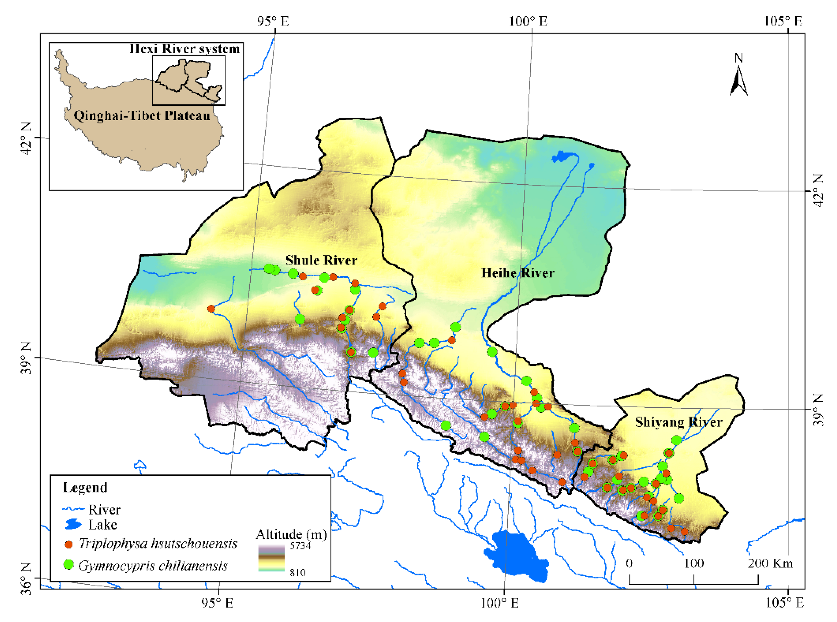
2.1. Occurrence Records

Occurrence records for G. chilianensis and T. hsutschouensis were exhaustively collected from published literature (including journal articles and theses), books, two online databases (list of references provided in Supplementary Material Text S1), and specimens deposited in the museum of Lanzhou University, mostly collected between 1955 and 2001. Existing records were further supplemented by our three field surveys across the Hexi River system from 2019 to 2021. We first checked and removed records with no, ambiguous, and duplicate geographical coordinates. Then, distribution data were further deleted using the SDMtoolbox analyses in ArcGIS 10.7 software (5 km spatial filter) to avoid overfitting of the model caused by spatial autocorrelation [41]. Finally, 46 and 47 distribution points of G. chilianensis and T. hsutschouensis were obtained, respectively, and marked in the study area (Figure 1); the data were then transformed into comma-delimited (CSV) forms to develop the MaxEnt model.

2.2. Current and Future Environmental Variables

In this study, four sets of factors related to climate (19 bioclimatic variables), topography (altitude and slope), food resources (net primary productivity), and human activities (human footprint) were considered (description of all environmental variables see Table 1). A total of 23 variables were included because they have well-illustrated effects on the fish species distributions [42,43].
Current (average of estimates for 1970–2000) and future climate factor data with a 2.5′ spatial resolution were downloaded from the WorldClim database [44]. Future climate data were used for the years 2050 (average of estimates for 2041–2060) and 2070 (average of estimates for 2061–2080) based on the Community Climate System Model version 4 (CCSM4) [45]. The best-fit model (i.e., CCSM4) for the study area was selected in advance by comparing the receiver operating characteristic (ROC) curve of four Global Circulation Models (GCMs; HadGEM2-CC, MPI-ESM-LR, MIROC-ESM, and CCSM4) that had demonstrated good performance in China [46]. The area under the ROC curve (AUC) values ranged from 0.5 to 1, with values above 0.9 suggesting that the accuracy of prediction reached the level of excellence [40,47]. The results showed that the only value above 0.9 was observed in the CCSM4 model based on the distribution records of G. chilianensis (Figure S1). We used two representative concentration pathways (RCPs), 2.6 and 8.5, representing the lowest (RCP2.6) and highest (RCP8.5) projected impacts of rising greenhouse gas concentrations on climate to test future changes in habitat suitability [48]. To maintain comparability of the models over the time series, the remaining three sets of factors (i.e., topography, food resources, and human activities) were applied jointly to the current and future distributions [49]. All environmental layers were extracted and clipped to the study area boundary, resampled to a spatial resolution of 1 km, subjected to the Albers Conical Equal Area Projection, and converted into ASCII files for constructing the models via ArcGIS.
To filter valid environmental data, we considered both the autocorrelation between environmental factors and their biological significance [50]. We first used all current environmental variables to develop the initial model and calculated the contribution of each variable to the model prediction via the Jackknife test already built into the Maxent model. Additionally, to avoid model overfitting and minimize multicollinearity between variables [51,52], the layers with high correlation (Pearson correlation coefficient, |r| ≥ 0.8) were discarded. In other words, when the |r| between two environmental variables was greater than 0.8, the one with the higher contribution in the initial model test was selected as the predictor. Eventually, eight environmental variables for both G. chilianensis and T. hsutschouensis were included for analysis: mean diurnal range (Bio2), isothermality (Bio3), mean temperature of the driest quarter (Bio9), annual precipitation (Bio12), precipitation of the driest period (Bio14), precipitation seasonality (Bio15), altitude (Alt), and slope (Slo).

2.3. MaxEnt Model Development

The distribution pattern of the target species was determined using MaxEnt 3.4.1 [39]. After importing valid species-presence points and data from the eight selected environmental variables, we reran the MaxEnt model. In our models, 75% of the sample data were randomly utilized for training, whereas 25% of the data were selected for testing. To ensure the stability of the model results, we repeated the operation 10-folds of Bootstrap. We calculated the habitat suitability response curves for each variable and determined the percent contributions of each variable to the target species habitat suitability model using the Jackknife test provided by MaxEnt. We selected the logistic distribution as the model output format for measuring the probability of species presence [53].
For model performance, the ROC curve was plotted, and the AUC was calculated to test the model’s accuracy. Threshold selection was based on maximizing the sum of sensitivity and specificity, which was repeated 10 times to attain average species’ habitat suitability threshold values [54]. The values above the threshold were considered suitable areas or suitability for species occurrence, and other values were considered unsuitable areas or unsuitability. Suitable (1) and unsuitable (0) habitats of the target species were divided and mapped using the artificial classification method in the reclassification tool of ArcGIS. To quantify the changes in species suitability under different climate change scenarios, the area of suitable habitats for the target species in the current and future distributions was calculated using the Spatial Analyst tool in the ArcGIS application.
To determine the spatial range shift of species over time, we narrowed the distribution range of suitable habitats to a single centroid and mapped its geographical sites in different periods and scenarios using the Mean Center method in the Spatial Statistics tool of the ArcGIS application [39,40,53].

3. Results

3.1. Model Evaluation

The average training AUC values under the current and future climate models were higher than 0.9 (Table 2, Figure S2), which indicated that the models for G. chilianensis and T. hsutschouensis were descriptive and sensitive. The results also showed that the MaxEnt model adequately simulated the relationship between the geographical distribution and selected environmental variables of the target species. Additionally, the AUC values suggested that models for T. hsutschouensis (all ≥ 0.936) for the current and future distributions showed slightly higher performances than those for G. chilianensis (all ≥ 0.925) (Table 2).

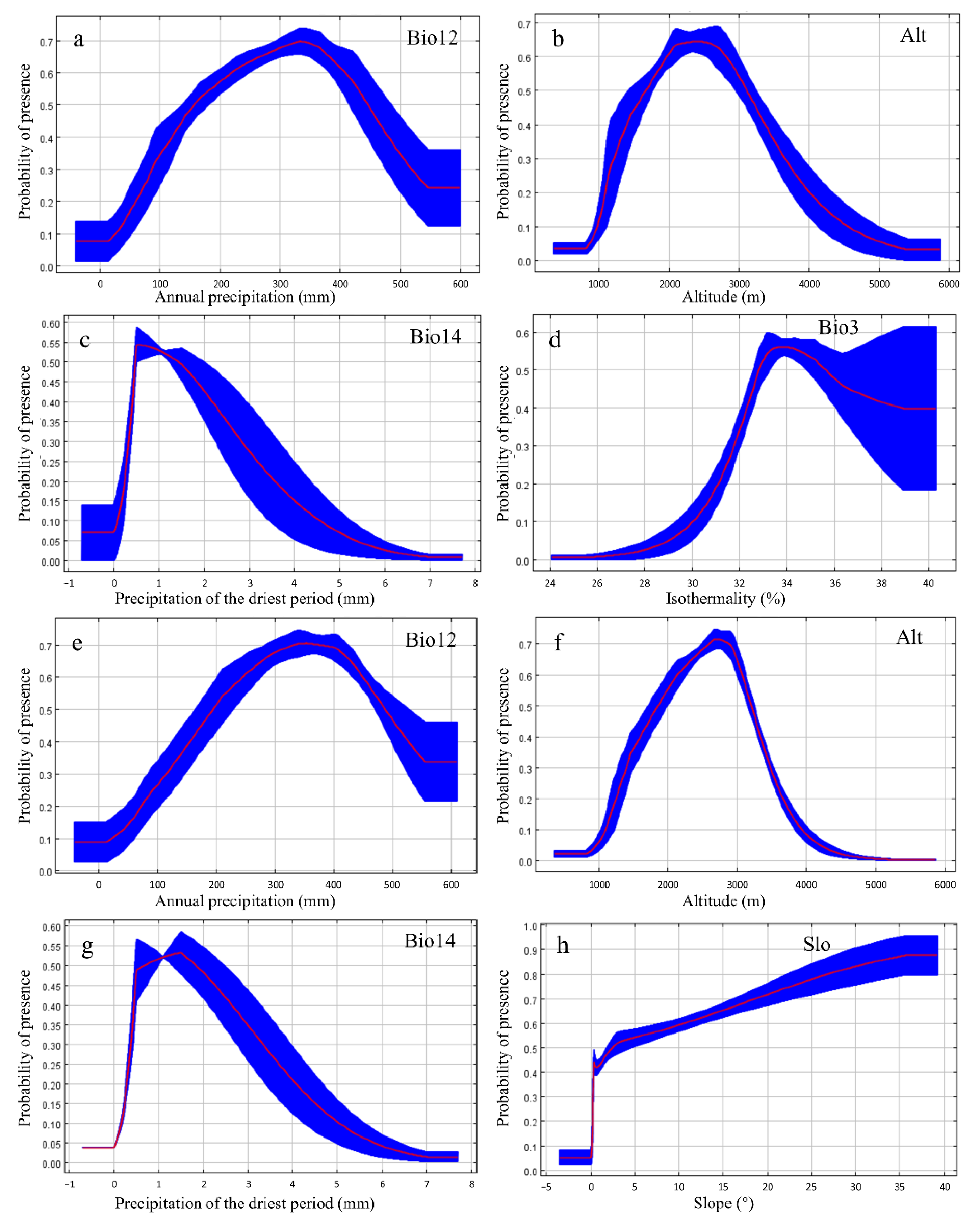
3.2. Important Variables

The Jackknife test results showed that the first four important variables affecting the suitability of G. chilianensis in the current model included Bio12 (contributing 35.8%), Alt (contributing 23.7%), Bio14 (contributing 20.0%), and Bio3 (contributing 10.6%), and the total contribution of these factors to building the model reached 90.1% (Table 3). The first four important variables influencing the suitability of T. hsutschouensis in the current model included Bio12 (contributing 38.7%), Alt (contributing 24.4%), Bio14 (contributing 19.1%), and Slo (contributing 8.0%), and the total contribution of these factors to building the model reached 90.2% (Table 3). We found that Bio12 and Alt were the most vital variables affecting the suitability of G. chilianensis (totally contributing 59.5%) and T. hsutschouensis (totally contributing 63.1%).
The response curves of the first four important variables with the habitat suitability of the target species in the climate scenario are shown in Figure 2. For G. chilianensis, the suitable range (probability of presence >0.5) of Bio12 was from 150 to 450 mm with optimal precipitation of 340 mm, Alt was from 1700 to 3100 m with an optimal altitude of 2400 m, Bio14 was from 0.4 to 1.5 mm with an optimal value of 0.5, and Bio3 was from 32.8 to 35.8% with an optimal value of 33.7%. For T. hsutschouensis, the suitable range of Bio12 was from 200 to 490 mm with optimal precipitation of 330 mm, Alt was from 1900 to 3200 m with optimal altitude of 2800 m, Bio14 was from 0.6 to 1.8 mm with an optimal value of 1.5, and Slo was higher than 2.5° with an optimal value of 35.8°. Among the common important environmental factors (i.e., Bio12, Alt and Bio14), G. chilianensis and T. hsutschouensis have similar suitability ranges.

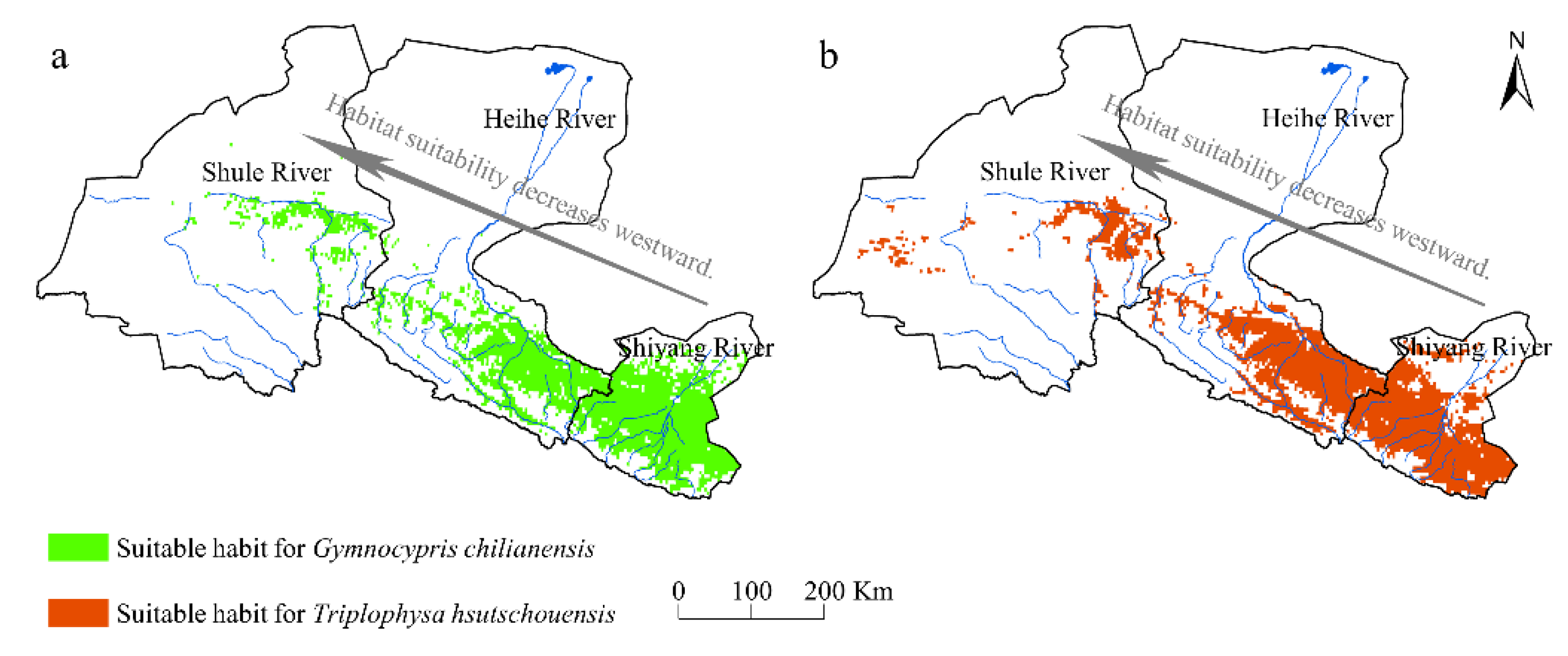
3.3. Current Suitability

A total of 46,580.3 km2 (14.4% of the study area) was computed as the suitable habitat area for G. chilianensis. A significant population of G. chilianensis was distributed in the Shiyang River, and other clusters were present in the middle and upper reaches of the Heihe River and Shule River (Figure 3a). Results indicated that suitable habitat decreased from east to west along the Hexi River system, with 24,212.2 km2 (52.0%), 17,686.1 km2 (37.9%), and 4680.3 km2 of suitable habitat concentrated in the Shiyang River, Heihe River, and Shule River, respectively.
For T. hsutschouensis, the suitable habitat area covered 48,751.8 km2 (15.0% of the background). Most parts of the Shiyang River, the middle and upper reaches of the Heihe River, and the middle reach of the Shule River supported the majority of the suitable habitat area of T. hsutschouensis (Figure 3b). Similar to the pattern of G. chilianensis, the three rivers harboring suitable habitats were the Shiyang River (22,189.1 km2, 45.5% of the total suitable habitat area), Heihe River (20,383.4 km2, 41.8%), and Shule River (6179.4 km2, 12.7%) in descending order from east to west along the Hexi River system.

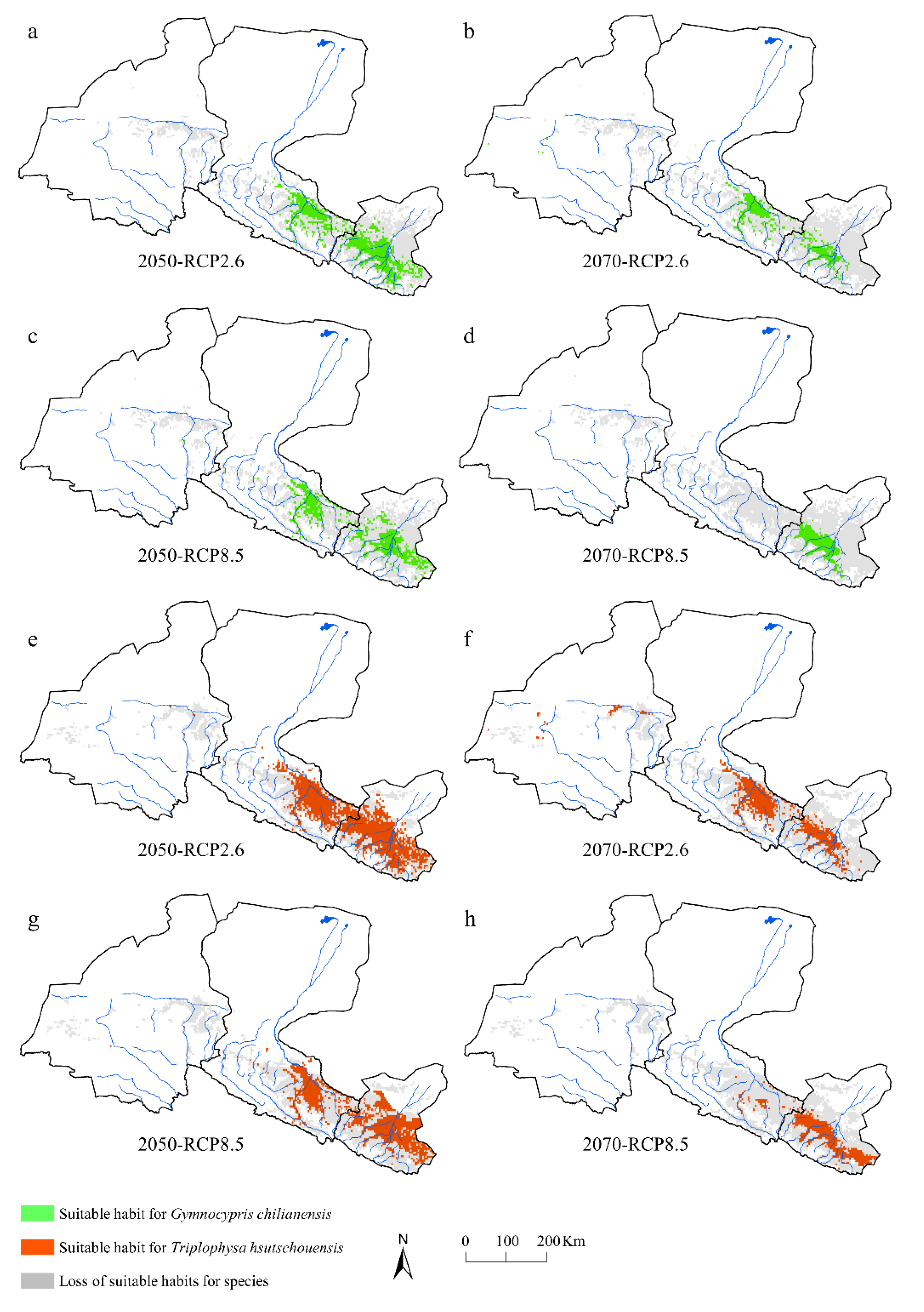
3.4. Predicted Changes in Suitability

A notable amount of suitable habitat contraction for G. chilianensis and T. hsutschouensis under both RCP2.6 and RCP8.5 for 2050 and 2070 can be tracked in Figure 4. For G. chilianensis: under RCP2.6, the suitable habitat for 2050 and 2070 was found to be decreased by 69.3% and 79.5%, respectively (Table 4, Figure 4a,b); under RCP8.5, the suitable habitat by 2050 and 2070 decreased by 75.9% and 88.5%, respectively (Table 4, Figure 4c,d). A high proportion of suitable habitat contraction was found in the Shule River. Suitable area contraction was also noticed in the middle and upper reaches of the Shiyang and Heihe Rivers.
Model results for T. hsutschouensis showed slightly less range contraction compared to G. chilianensis under future climate change scenarios (2050 and 2070) under both RCP2.6 and RCP8.5. A 45.1% and 69.2% loss of suitable habitat was predicted for 2050 and 2070 under RCP2.6, respectively (Table 4, Figure 4e,f), and 61.2% and 82.2% by 2050 and 2070 under RCP8.5, respectively (Table 4, Figure 4g,h). A noticeable amount of unsuitable habitat was found in the Shule River. The suitable habitat of T. hsutschouensis was scattered in the upper reaches of the Shiyang River and Heihe River. The results indicated a potential threat to the habitat suitability of G. chilianensis and T. hsutschouensis in the Hexi River system in the future.

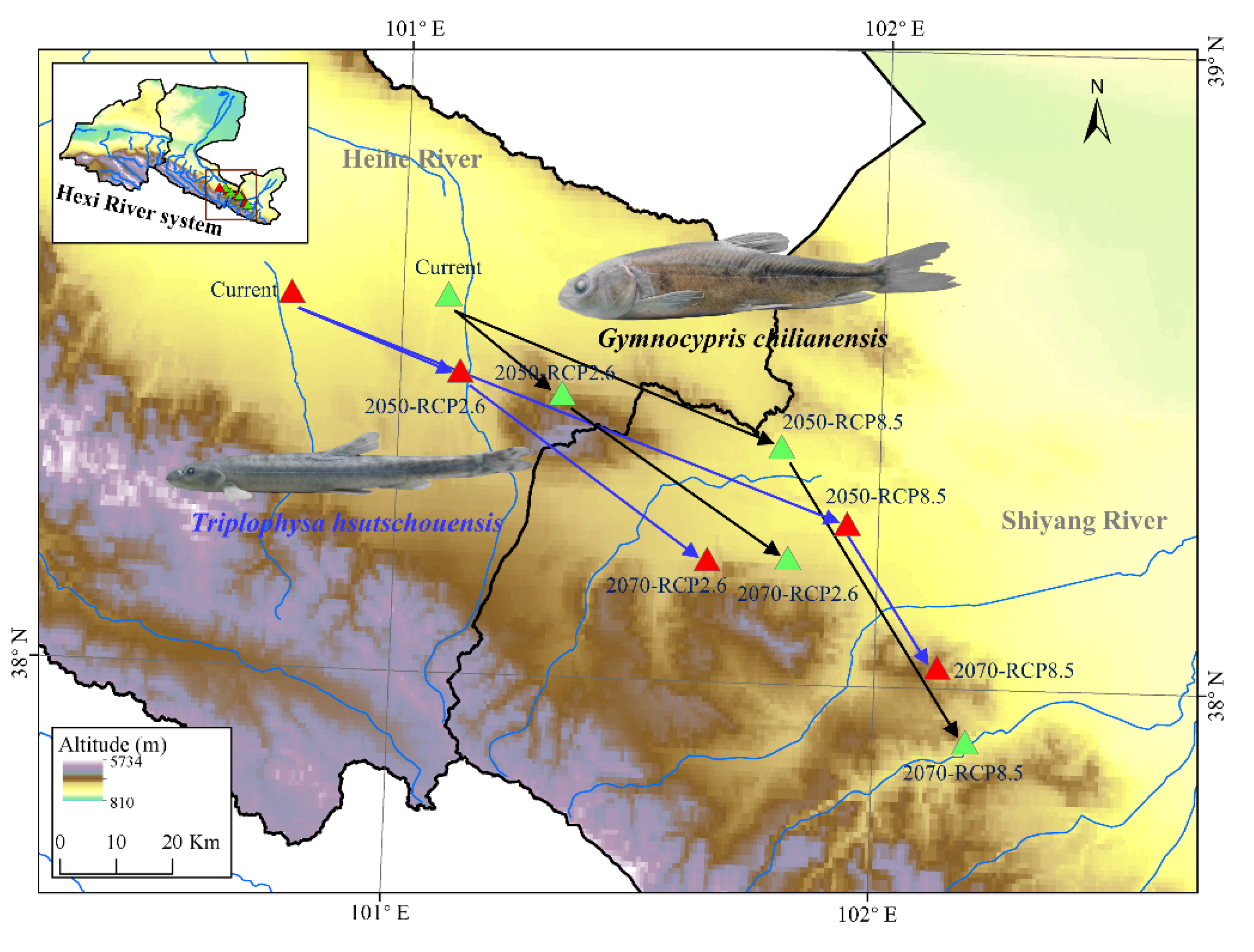
3.5. Distribution Center Change

Figure 5 shows the shifts in the centroid position of suitable habitat for G. chilianensis and T. hsutschouensis. Under future climate change scenarios, the centers of suitable habitat for the two target species were predicted to shift eastward from the Heihe River to the Shiyang River and to high-altitude areas in the southeast. This range shift was predicted to be more pronounced for G. chilianensis than for T. hsutschouensis.

4. Discussion

4.1. Variable Influences

Our results highlighted that environmental variables dependent on precipitation and topography were the major predictors that influence the suitable habitat of G. chilianensis and T. hsutschouensis. However, some studies on the QTP showed that temperature plays a more important role than precipitation in climate factors [55]. Because of residing in arid and semiarid regions of northwestern China, the target species are highly sensitive to variables related to precipitation [56], especially in the driest month, including annual precipitation (Bio12) and precipitation of the driest month (Bio14). Our results revealed similar predictor variables and habitat suitability values for both species, perhaps attributable to the species’ similarities in habitat preference (e.g., running water, benthopelagic) and feeding habits (i.e., omnivory) [57].
Annual precipitation and altitude were found to be the two most significant contributors to predicting the suitable habitat of the target species. The response curve for increased annual precipitation predicted an initial increase in habitat suitability for both species, which peaked and then decreased with continued increases in annual precipitation. Higher annual precipitation most likely provides more suitable conditions (e.g., food resources) for survival [58]. To adapt to food shortages on the plateau, G. chilianensis and T. hsutschouensis must feed on algae with low nutrient contents on the surfaces of mud or rocks (i.e., scrape-feeding behavior) [29]. Precipitation is, in a sense, a variable representing runoff. Increases in annual precipitation increase runoff, thus supplying more nutrients [59]. However, heavy precipitation events can mobilize sediment, which can destroy spawning grounds and prevent successful egg and larval development due to increased scouring effects [60,61]. As G. chilianensis and T. hsutschouensis grow very slowly, taking 9–10 years to reach approximately 500 g, stocks did not easily recover from habitat destruction and overexploitation in the short term [29]. Therefore, from the response curve of Bio12 (Figure 2a,e), there is a clear signal of an adverse effect of a continuous increase in annual precipitation on the habitat suitability for G. chilianensis and T. hsutschouensis.
Altitude is the second-best predictor. We found that the suitable range for G. chilianensis and T. hsutschouensis peaked at mid-elevations (the former and the latter were 2400 and 2800 m, respectively, Figure 2b,f). Energy and area hypotheses are often used to explain this suitability distribution pattern. Energy hypotheses, such as the water–energy dynamic hypothesis, claim that temperature (energy) decreases and annual precipitation (water) increases with increasing altitude for the whole mountain, thus forming the most suitable distribution area at mid-altitude [56,62]. Area hypotheses, such as the mid-domain effect, assert that if the ranges of the species are randomly distributed within a bounded domain, then more suitable ranges will occur near the middle of the domain than at the edges [63,64]. Similar studies on Tibetan fish reported identical results (e.g., Schizothoracinae [65] and Triplophysa [55]). Hence, the suitability distribution of native fish that peaked at mid-altitudes is more likely to be a general pattern on the QTP and adjacent areas.

4.2. Current Distribution Characteristics

Our results demonstrated that the currently suitable habitat areas for G. chilianensis and T. hsutschouensis decreased from east to west along the Shiyang, Heihe, and Shule Rivers. On the one hand, from an ecological perspective, the environmental conditions (e.g., precipitation and temperature) of the Hexi River system become harsher from east to west, driving the geographical decay of the suitability of the target species [17,22]. This is evident from a study of G. chilianensis morphology [30], which showed a geographical cline in the character of the horny ridge at the inner margin of the lower jaw from east to west along the Hexi River system: a weak horny ridge was presented in the Shiyang River population, trending towards modest in the Heihe River population and strong in the Shule River population [30,31]. This exhibited pattern was due to ecological adaptation to different habitat environments, with the increasingly poor food resources attributed to drier conditions, less rainfall, and higher temperatures from the Shiyang River to the Shule River [30]. On the other hand, from an evolutionary perspective, Feng et al. [32] demonstrated that T. hsutschouensis first appeared in the Shiyang River (i.e., ancestral population region) and then gradually expanded westward along the Heihe River and Shule River by phylogenetic analysis. Additionally, similar studies were reported by Zhao et al. [31] for G. chilianensis. Historical hypotheses argue that ancestral populations allow for higher species suitability [66]. Ancestral populations have more time to accumulate mutations (i.e., increasing genetic diversity), which might provide the potential for future adaptive responses to habitat and climate. Thus, ecological and evolutionary factors may jointly shape our findings that the Shiyang River was the region with the highest population suitability, after which it gradually reduced westward along the Heihe and Shule Rivers.

4.3. Future Changes

Our results indicated that loss of suitable habitat and range shifts were the most significant impacts of the increasing intensity of climate change on G. chilianensis and T. hsutschouensis. These findings are in accordance with the general understanding of the response of biodiversity to anthropogenic climate change [67,68]. Under predicted climate change scenarios (RCP2.6 and RCP8.5), increasing extreme weather events in the Hexi River system, such as ice collapse and debris flow and heavy precipitation, destroy fish habitats by breaking down their spawning grounds [69]. Higher temperatures and rising precipitation that falls as rain rather than snow lead to melting ice at high-altitude regions of the Hexi River system, meaning less meltwater will flow to the three inland rivers, leaving less suitable habitat for plateau fish in the future [70]. In addition, G. chilianensis and T. hsutschouensis only exist in narrow habitats on the QTP, suffer from natural disadvantages of slow growth, and require specific environmental conditions, such as lotic and cold water. The populations of the three rivers have become isolated from each other due to previous geological and climatic events, thus impeding exchanges between populations [22]. Some other factors that are not included in the model, such as the invasion of alien species and the construction of dams [4,71], might limit their suitability for the species. Therefore, these threats are likely to drive much of the predicted reduction in habitat suitability under future climate change scenarios, thus causing severe consequences for G. chilianensis and T. hsutschouensis. These stressors force G. chilianensis and T. hsutschouensis to return to the ancestral population region (i.e., Shiyang River) and shift to high-altitude areas, which harbor suitable conditions for survival and colonization, such as relatively low temperature, suitable precipitation, more rechargeable meltwater and lower densities of anthropogenic activity. This finding also confirms that the ancestral population region provides a stable environment over time, allowing the preservation of species through successive periods of climate change [72]. Additionally, compared to terrestrial groups in the Hexi region (e.g., Pseudois nayaur and Moschus chrysogaster [73]), G. chilianensis and T. hsutschouensis are more vulnerable to climate change due to limited freshwater dispersal pathways, mountain barriers, and expansive lands [74]. Dispersal limitation is also a reason that accelerated plateau climate change is taking a large toll on these species’ habitat suitability.
Although precipitation was a better predictor than temperature, the Jackknife test observed that isothermality (Bio3) was the fourth-best predictor for the suitable habitat of G. chilianensis, while it was the fifth-best predictor for that of T. hsutschouensis. Isothermality is an index derived from the ratio of the mean diurnal temperature range (Bio2) and annual temperature range (Bio7), and the higher the value is, the more similar the diurnal and annual temperature ranges are [75]. Temperature is also an important climatic factor that shapes the distribution of fish by directly affecting fish growth and reproduction. Being plateau cold fish, G. chilianensis was more sensitive to isothermality dependent on temperature than T. hsutschouensis due to different internal physiological and biochemical responses to plateau conditions [76,77,78], resulting in greater changes, including the loss of suitable area and movement range of the distribution center, observed in the former under future accelerated climate warming. Another reason why G. chilianensis is more vulnerable to climate change is related to the phylogenetic history and genetic diversity of the target species. Ancestral populations tend to have higher genetic diversity, which could potentially lead to the increased adaptive capacity of the population [79]. Reports [31,32] showed that G. chilianensis in the three rivers had a shorter phylogenetic history and lower genetic diversity than T. hsutschouensis, which might indicate that G. chilianensis could be more vulnerable to climate change.

4.4. Conservation

This study predicts that future climate change poses serious threats to the persistence of endemic plateau fish. Fishery managers and conservation institutions must take effective measures to relieve the pressure of accelerated climate change. Unfortunately, existing conservation efforts are mainly focused on reducing fishing pressure and promoting the conservation of populations in selected areas [80]. Including the effects of future climate change in systematic conservation plans is therefore urgently needed. For example, priority areas for fish conservation should be evaluated based on multifaceted components of biodiversity (e.g., taxonomic diversity, functional diversity, genetic diversity, and phylogenetic diversity), human impact, and vulnerability or suitability to climate change [81,82]. In addition, in the face of equally pressing issues from accelerated plateau climate change and the multiple biological roles it plays in the Hexi River system (e.g., indicator species and the only endemic species of Triplophysa), T. hsutschouensis, similar to G. chilianensis, should also be considered as a key protected species in Gansu Province in the long term to enhance conservation awareness. A joint scheduling plan of the reservoir group is expected to address the challenges of heavy precipitation and extreme weather events, as well as less meltwater. Sites of the reservoir group (including reservoirs and hydropower stations) were marked in Figure S3 through surveys and visits to water authorities. Firstly, based on the historical water volume and precipitation pattern of the river during abundant, flat and dry periods, combined with the demand for fish spatial activities and reproduction conditions (e.g., water quantity, flow rate, and temperature), a reasonable ecological flow rate should be calculated. Then, the number of high and low flow pulses occurring should be kept within reasonable limits by the reservoir complex (i.e., the joint scheduling plan of the reservoir group) to ensure a relatively constant water quantity, especially during the fish reproduction period [83]. Through this effort, the impact of less ice-snow melting water flowing to inland rivers on fish life histories caused by heavy precipitation is expected to be mitigated.

4.5. Limitations

Despite providing valuable insights into understanding the effects of climate change on the suitable habitat of plateau fish, we must acknowledge that our findings have several limitations. First, our results are subject to some uncertainty. Due to the instability of a single GCMs, the absence of hydrological factors, and the difference in investigating time from heterogeneous sources (e.g., published literature, books, museum, and field surveys), our findings might overestimate or underestimate the goodness of the model and the range of suitable habitats for the target species to some extent [84,85,86]. Second, the MaxEnt model takes into account a limited number of variables. The distribution of suitable habitats for fish species is shaped by multiple factors, such as interspecies interactions, dispersal ability, and the evolutionary history of fish [26,87]. Nevertheless, it is often challenging to quantify and input all the influencing factors into the model. Third, the coarse-resolution GCMs at regional scales might have influenced our results. GCMs provide global large-scale information for the construction of climate change. However, when studies are conducted at local and regional scales, GCMs produce large biases in the prediction of climate change due to the coarse resolution [88]. Larger-scale environmental variables can be developed into small-scale finer quantities with the help of downscaling methods (e.g., dynamic downscaling and statistical downscaling) [89]. The mismatch between the input variables and the spatial and temporal scales of the evaluated objects may significantly reduce the accuracy of climate change impact assessment [90]. Thus, downscaling approaches need to be applied at finer spatial scales in future studies. Finally, our analysis did not consider model calibration. Our estimates of future change relied on a comparison of future changes in climate scenarios with results based on purely historical observations. However, GCMs have their own systematic uncertainties in representing local climates over historical periods [91]. Consequently, the uncertainties obtained theoretically would be transmitted to future periods. Models calibrated to real historical observations should be simulated against GCMs outputs for the same period, and the results obtained are the basis and reference conditions for assessing changes under climate scenarios; thus, future changes need to be compared with historical periods based on GCM outputs to eliminate the uncertainties from the GCMs [92,93]. Nevertheless, it is often challenging to fill these various knowledge gaps due to real historical data deficiency and the limitations of methodologies. Therefore, future studies should incorporate multimodel, downscaling methods and the calibrated model to better understand the effects of accelerated plateau climate change on the distributional range of plateau fish.

5. Conclusions

We constructed SDMs for G. chilianensis and T. hsutschouensis using the MaxEnt algorithm based on a comprehensive collection of presence records and environmental variables. The model predicted currently suitable areas and future changes for the species in light of accelerated plateau climate change. We demonstrate that different plateau fish have similarities and differences in their responses to climate change. Our study provides a representative case in which accelerated climate change on the QTP has severe consequences, potentially leading to population extirpation and, for these two endemic plateau species, possible species extinctions. Hence, the effects of climate change must be incorporated into the integrated conservation plans for fish species on the QTP and its adjacent areas.

Supplementary Materials

The following supporting information can be downloaded at: https://www.mdpi.com/article/10.3390/d14100877/s1, Text S1: The data source of distribution information for Gymnocypris chilianensis and Triplophysa hsutschouensis in the Hexi River system, the Qinghai–Tibetan Platea; Figure S1: Receiver operating characteristic (ROC) curve verification of distribution of Gymnocypris chilianensis based on four Global Circulation Models (GCMs; HadGEM2-CC, MPI-ESM-LR, MI-ROC-ESM and CCSM4). The red (training) line shows the “fit” of the model to the training data. The blue (testing) line indicates the fit of the model to the testing data and is the real test of the model’s predictive power; Figure S2: Receiver operating characteristic (ROC) curve verification of distribution of Gymnocypris chilianensis (a–e) and Triplophysa hsutschouensis (f–j) under different climate scenarios predicted by the Maxent model; Figure S3: Reservoir group (reservoir and hydropower station) in the Hexi River system. Data were obtained through surveys and visits to water authorities.

Author Contributions

D.H. and Z.C. conceived the ideas and performed the analyses. Z.W. and Z.C. took part in the field works and collected the data. L.C. and Z.C. contributed analysis tools. Z.C. led the writing. All authors have read and agreed to the published version of the manuscript.

Funding

This research was funded by the Second Tibetan Plateau Scientific Expedition Program (2019QZKK05010102), Lanzhou University Student’s Innovation and Entrepreneurship Action Plan Program (20220180044).

Institutional Review Board Statement

Not applicable.

Data Availability Statement

Not applicable.

Acknowledgments

We extend our sincere gratitude to the editor and anonymous reviewers for their constructive comments that helped to improve the manuscript. We also give our thanks to Ningning Wang, Yuying He, Peijia Li, and Yiqing Sheng (School of Life Sciences, Lanzhou University) for data handling.

Conflicts of Interest

The authors declare no conflict of interest.

References

  1. Mooney, H.; Larigauderie, A.; Cesario, M.; Elmquist, T.; Hoegh-Guldberg, O.; Lavorel, S.; Mace, G.M.; Palmer, M.; Scholes, R.; Yahara, T. Biodiversity, climate change, and ecosystem services. Curr. Opin. Environ. Sustain. 2009, 1, 46–54. [Google Scholar] [CrossRef]
  2. Barnosky, A.D.; Matzke, N.; Tomiya, S.; Wogan, G.O.U.; Swartz, B.; Quental, T.B.; Marshall, C.; McGuire, J.L.; Lindsey, E.L.; Maguire, K.C.; et al. Has the Earth’s sixth mass extinction already arrived? Nature 2011, 471, 51–57. [Google Scholar] [CrossRef] [PubMed]
  3. IPCC. Climate Change 2014: Synthesis Report. In Contribution of Working Groups I, II and III to the Fifth Assessment Report of the Intergovernmental Panel on Climate Change; IPCC: Geneva, Switzerland, 2014; 151p. [Google Scholar]
  4. Liu, C.; Comte, L.; Xian, W.; Chen, Y.; Olden, J.D. Current and projected future risks of freshwater fish invasions in China. Ecography 2019, 42, 2074–2083. [Google Scholar] [CrossRef]
  5. Lenoir, J.; Svenning, J.C. Climate-related range shifts–a global multidimensional synthesis and new research directions. Ecography 2015, 38, 15–28. [Google Scholar] [CrossRef]
  6. Urban, M.C. Accelerating extinction risk from climate change. Science 2015, 348, 571–573. [Google Scholar] [CrossRef] [Green Version]
  7. Comte, L.; Olden, J.D. Climatic vulnerability of the world’s freshwater and marine fishes. Nat. Clim. Change 2017, 7, 718–722. [Google Scholar] [CrossRef]
  8. Dudgeon, D.; Arthington, A.H.; Gessner, M.O.; Kawabata, Z.I.; Knowler, D.J.; Lévêque, C.; Naiman, R.J.; Prieur-Richard, A.H.; Soto, D.; Stiassny, M.L.J.; et al. Freshwater biodiversity: Importance, threats, status and conservation challenges. Biol. Rev. 2007, 81, 163–182. [Google Scholar] [CrossRef]
  9. Avaria-Llautureo, J.; Venditti, C.; Rivadeneira, M.M.; Inostroza-Michael, O.; Rivera, R.J.; Hernández, C.E.; Canales-Aguirre, C.B. Historical warming consistently decreased size, dispersal and speciation rate of fish. Nat. Clim. Change 2021, 11, 787–793. [Google Scholar] [CrossRef]
  10. Knouft, J.H.; Ficklin, D.L. The potential impacts of climate change on biodiversity in flowing freshwater systems. Annu. Rev. Ecol. Evol. Syst. 2017, 48, 111–133. [Google Scholar] [CrossRef]
  11. Barbarossa, V.; Bosmans, J.; Wanders, N.; King, H.; Bierkens, M.F.P.; Huijbregts, M.A.J.; Schipper, A.M. Threats of global warming to the world’s freshwater fishes. Nat. Commun. 2021, 12, 1701. [Google Scholar] [CrossRef]
  12. Nogués-Bravo, D.; Araújo, M.B.; Errea, M.P.; Martínez-Rica, J.P. Exposure of global mountain systems to climate warming during the 21st century. Glob. Environ. Change 2007, 17, 420–428. [Google Scholar] [CrossRef]
  13. Mountain Research Initiative EDW Working Group. Elevation-dependent warming in mountain regions of the world. Nat. Clim. Change 2015, 5, 424–430. [Google Scholar] [CrossRef] [Green Version]
  14. Klanderud, K.; Totland, Ø. Simulated climate change altered dominance hierarchies and diversity of an alpine biodiversity hotspot. Ecology 2005, 86, 2047–2054. [Google Scholar] [CrossRef] [Green Version]
  15. Jay, F.; Manel, S.; Alvarez, N.; Durand, E.Y.; Thuiller, W.; Holderegger, R.; Taberlet, P.; François, O. Forecasting changes in population genetic structure of alpine plants in response to global warming. Mol. Ecol. 2012, 21, 2354–2368. [Google Scholar] [CrossRef] [PubMed]
  16. Liu, X.; Chen, B. Climatic warming in the Tibetan Plateau during recent decades. Int. J. Climatol. 2000, 20, 1729–1742. [Google Scholar] [CrossRef]
  17. Liu, J.; Xin, Z.; Huang, Y.; Yu, J. Climate suitability assessment on the Qinghai-Tibet Plateau. Sci. Total Environ. 2022, 816, 151653. [Google Scholar] [CrossRef] [PubMed]
  18. Qu, Y.H.; Ericson, P.G.P.; Lei, F.M.; Li, S.H. Postglacial colonization of the Tibetan plateau inferred from the matrilineal genetic structure of the endemic red-necked snow finch, Pyrgilauda ruficollis. Mol. Ecol. 2005, 14, 1767–1781. [Google Scholar] [CrossRef]
  19. Zhang, Q.; Chiang, T.Y.; George, M.; Liu, J.Q.; Abbott, R.J. Phylogeography of the Qinghai-Tibetan Plateau endemic Juniperus przewalskii (Cupressaceae) inferred from chloroplast DNA sequence variation. Mol. Ecol. 2005, 14, 3513–3524. [Google Scholar] [CrossRef]
  20. Qi, D.; Guo, S.; Zhao, X.; Yang, J.; Tang, W. Genetic diversity and historical population structure of Schizopygopsis pylzovi (Teleostei: Cyprinidae) in the Qinghai-Tibetan Plateau. Freshw. Biol. 2007, 52, 1090–1104. [Google Scholar] [CrossRef]
  21. Zhao, K.; Duan, Z.; Yang, G.; Peng, Z.; He, S.; Chen, Y. Origin of Gymnocypris przewalskii and phylogenetic history of Gymnocypris eckloni (Teleostei: Cyprinidae). Prog. Nat. Sci. 2007, 17, 520–528. [Google Scholar]
  22. Chen, Z.; Luo, L.; Wang, Z.; He, D.; Zhang, L. Diversity and distribution of fish in the Qilian Mountain Basin. Biodivers. Data J. 2022, 10, e85992. [Google Scholar] [CrossRef]
  23. Feng, S.W. Evolution of Hexi water system in Gansu. J. Lanzhou Univ. Nat. Sci. 1981, 17, 125–129. [Google Scholar]
  24. Li, J.J. Discussion of the recent age and the quaternary glaciation of Qilian Mountains. J. Lanzhou Univ. Nat. Sci. 1963, 13, 77–86. [Google Scholar]
  25. Li, J.J.; Fang, X.M.; Pan, B.T.; Zhao, Z.J.; Song, Y.G. Late Cenozoic intensive uplift of Qinghai-Xizang plateau and its impacts on environments in surrounding area. Quat. Sci. 2001, 21, 381–391. [Google Scholar]
  26. He, D.; Sui, X.; Sun, H.; Tao, J.; Ding, C.; Chen, Y.; Chen, Y. Diversity, pattern and ecological drivers of freshwater fish in China and adjacent areas. Rev. Fish Biol. Fish. 2020, 30, 387–404. [Google Scholar] [CrossRef]
  27. Zhao, T.Q. Fish-fauna and zoogeographical division of Hexi-Alashan region, the northwest China. Acta Zool. Sin. 1991, 37, 153–167. [Google Scholar]
  28. Wang, X.T. Vertebrate Fauna of Gansu; Gansu Science and Technology Press: Lanzhou, China, 1991; pp. 35–36, 102–105. [Google Scholar]
  29. Wu, Y.F.; Wu, C.Z. The Fishes of the Qinghai-Xizang Plateau; Sichuan Publishing House of Science and Technology: Chengdu, China, 1992; pp. 190–192, 446–448. [Google Scholar]
  30. Zhao, T.Q. On the taxonomic problem of Gymnocpris eckloni Herzenstein. La Anim. Mondo 1986, 3, 49–55. [Google Scholar]
  31. Zhao, K.; Duan, Z.; Peng, Z.; Gan, X.; Zhang, R.; He, S.; Zhao, X. Phylogeography of the endemic Gymnocypris chilianensis (Cyprinidae): Sequential westward colonization followed by allopatric evolution in response to cyclical Pleistocene glaciations on the Tibetan Plateau. Mol. Phylogenet. Evol. 2011, 59, 303–310. [Google Scholar] [CrossRef]
  32. Feng, C.; Zhou, W.; Tang, Y.; Gao, Y.; Chen, J.; Tong, C.; Liu, S.; Wanghe, K.; Zhao, K. Molecular systematics of the Triplophysa robusta (Cobitoidea) complex: Extensive gene flow in a depauperate lineage. Mol. Phylogenet. Evol. 2019, 132, 275–283. [Google Scholar] [CrossRef]
  33. Wang, T.; Zhang, Y.P.; Yang, Z.Y.; Liu, Z.; Du, Y.Y. DNA barcoding reveals cryptic diversity in the underestimated genus Triplophysa (Cypriniformes: Cobitidae, Nemacheilinae) from the northeastern Qinghai-Tibet Plateau. BMC Evol. Biol. 2020, 20, 151. [Google Scholar] [CrossRef]
  34. Quan, J.; Zhao, G.; Li, L.; Zhang, J.; Luo, Z.; Kang, Y.; Liu, Z. Phylogeny and genetic diversity reveal the influence of Qinghai-Tibet Plateau uplift on the divergence and distribution of Gymnocypris species. Aquat. Sci. 2021, 83, 6. [Google Scholar] [CrossRef]
  35. Allouche, O.; Tsoar, A.; Kadmon, R. Assessing the accuracy of species distribution models: Prevalence, kappa and the true skill statistic (TSS). J. Appl. Ecol. 2006, 43, 1223–1232. [Google Scholar] [CrossRef]
  36. Pearson, R.G. Species’ distribution modeling for conservation educators and practitioners. Lessons Conserv. 2010, 3, 54–89. [Google Scholar]
  37. Guisan, A.; Zimmermann, N.E. Predictive habitat distribution models in ecology. Ecol. Modell. 2000, 135, 147–186. [Google Scholar] [CrossRef]
  38. Elith, J.; Leathwick, J.R. Species distribution models: Ecological explanation and prediction across space and time. Annu. Rev. Ecol. Evol. Syst. 2009, 40, 677–697. [Google Scholar] [CrossRef]
  39. Phillips, S.J.; Anderson, R.P.; Schapire, R.E. Maximum entropy modeling of species geographic distributions. Ecol. Modell. 2006, 190, 231–259. [Google Scholar] [CrossRef] [Green Version]
  40. Phillips, S.J.; Dudik, M. Modeling of species distributions with Maxent: New extensions and a comprehensive evaluation. Ecography 2008, 31, 161–175. [Google Scholar] [CrossRef]
  41. Williams, P.H.; Margules, C.R.; Hilbert, D.W. Data requirements and data sources for biodiversity priority area selection. J. Biosci. 2002, 27, 327–338. [Google Scholar] [CrossRef]
  42. Li, Y.; Qin, T.; Tun, Y.Y.; Chen, X. Fishes of the Irrawaddy River: Diversity and conservation. Aquat. Conserv. 2021, 31, 1945–1955. [Google Scholar] [CrossRef]
  43. Zhang, C.; Zhu, R.; Sui, X.; Li, X.; Chen, Y. Understanding patterns of taxonomic diversity, functional diversity, and ecological drivers of fish fauna in the Mekong River. Glob. Ecol. Conserv. 2021, 28, e01711. [Google Scholar] [CrossRef]
  44. WorldClim. Free Climate Data for Ecological Modeling and GIS. Available online: https://www.worldclim.org/ (accessed on 25 May 2022).
  45. Hijmans, R.J.; Cameron, S.E.; Parra, J.L.; Jones, P.G.; Jarvis, A. Very high resolution interpolated climate surfaces for global land areas. Int. J. Climatol. 2005, 25, 1965–1978. [Google Scholar] [CrossRef]
  46. Chen, L.; Frauenfeld, O.W. Surface air temperature changes over the twentieth and twenty-first centuries in China simulated by 20 CMIP5 models. J. Clim. 2014, 27, 3920–3937. [Google Scholar] [CrossRef]
  47. Hu, W.; Wang, Y.; Dong, P.; Zhang, D.; Yu, W.; Ma, Z.; Chen, G.; Liu, Z.; Du, J.; Chen, B.; et al. Predicting potential mangrove distributions at the global northern distribution margin using an ecological niche model: Determining conservation and reforestation involvement. For. Ecol. Manag. 2020, 478, 118517. [Google Scholar] [CrossRef]
  48. Meinshausen, M.; Smith, S.J.; Calvin, K.; Daniel, J.S.; Kainuma, M.L.T.; Lamarque, J.F.; Matsumoto, K.; Montzka, S.A.; Raper, S.C.B.; Riahi, K.; et al. The RCP greenhouse gas concentrations and their extensions from 1765 to 2300. Clim. Change 2011, 109, 213–241. [Google Scholar] [CrossRef] [Green Version]
  49. Sreekumar, E.R.; Nameer, P.O. A MaxEnt modelling approach to understand the climate change effects on the distributional range of White-bellied Sholakili Sholicola albiventris (Blanford, 1868) in the Western Ghats, India. Ecol. Inform. 2022, 70, 101702. [Google Scholar] [CrossRef]
  50. Fourcade, Y.; Engler, J.O.; Rödder, D.; Secondi, J. Mapping species distributions with MaxEnt using a geographically biased sample of presence data: A performance assessment of methods for correcting sampling bias. PLoS ONE 2014, 9, e97122. [Google Scholar] [CrossRef] [Green Version]
  51. Elith, J.; Phillips, S.J.; Hastie, T.; Dudík, M.; Chee, Y.E.; Yates, C.J. A statistical explanation of MaxEnt for ecologists. Divers. Distrib. 2010, 17, 43–57. [Google Scholar] [CrossRef]
  52. Merow, C.; Smith, M.J.; Silander, J.A., Jr. A practical guide to MaxEnt for modeling species’ distributions: What it does, and why inputs and settings matter. Ecography 2013, 36, 1058–1069. [Google Scholar] [CrossRef]
  53. Phillips, S.J.; Anderson, R.P.; Dudík, M.; Schapire, R.E.; Blair, M.E. Opening the black box: An open-source release of Maxent. Ecography 2017, 40, 887–893. [Google Scholar] [CrossRef]
  54. Liu, C.; White, M.; Newell, G. Selecting thresholds for the prediction of species occurrence with presence-only data. J. Biogeogr. 2013, 40, 778–789. [Google Scholar] [CrossRef]
  55. Feng, C.; Wu, Y.; Tian, F.; Tong, C.; Tang, Y.; Zhang, R.; Li, G.; Zhao, K. Elevational diversity gradients of Tibetan loaches: The relative roles of ecological and evolutionary processes. Ecol. Evol. 2017, 7, 9970–9977. [Google Scholar] [CrossRef] [Green Version]
  56. Hawkins, B.A.; Field, R.; Cornell, H.V.; Currie, D.J.; Guégan, J.F.; Kaufman, D.M.; Kerr, J.T.; Mittelbach, G.G.; Oberdorff, T.; O’Brien, E.M.; et al. Energy, water, and broad-scale geographic patterns of species richness. Ecology 2003, 84, 3105–3117. [Google Scholar] [CrossRef] [Green Version]
  57. Froese, R.; Pauly, D.; FishBase. World Wide Web Electronic Publication. Available online: http://www.fishbase.org,version (accessed on 2 August 2022).
  58. Hu, Y.; Fan, H.; Chen, Y.; Chang, J.; Zhan, X.; Wu, H.; Zhang, B.; Wang, M.; Zhang, W.; Yang, L.; et al. Spatial patterns and conservation of genetic and phylogenetic diversity of wildlife in China. Sci. Adv. 2021, 7, eabd5725. [Google Scholar] [CrossRef] [PubMed]
  59. Kang, B.; Huang, X. Mekong fishes: Biogeography, migration, resources, threats, and conservation. Rev. Fish. Sci. Aquac. 2022, 30, 170–194. [Google Scholar] [CrossRef]
  60. Bruton, M.N. The effects of suspensoids on fish. Hydrobiologia 1985, 125, 221–241. [Google Scholar] [CrossRef]
  61. Hauer, C.; Leitner, P.; Unfer, G.; Pulg, U.; Habersack, H.; Graf, W. The role of sediment and sediment dynamics in the aquatic environment. In Riverine Ecosystem Management; Schmutz, S., Sendzimir, J., Eds.; Springer: Cham, Switzerland, 2018; Volume 8, pp. 151–169. [Google Scholar]
  62. O’Brien, E.M. Climatic gradients in woody plant species richness: Towards an explanation based on an analysis of Southern Africa’s woody flora. J. Biogeogr. 1993, 20, 181–198. [Google Scholar] [CrossRef]
  63. Colwell, R.K.; Hurtt, G.C. Nonbiological gradients in species richness and a spurious Rapoport effect. Am. Nat. 1944, 144, 570–595. [Google Scholar] [CrossRef]
  64. Colwell, R.K.; Lees, D.C. The mid-domain effect: Geometric constraints on the geography of species richness. Trends Ecol. Evol. 2000, 15, 70–76. [Google Scholar] [CrossRef]
  65. Li, J.; He, Q.; Hua, X.; Zhou, J.; Xu, H.; Chen, J.; Fu, C. Climate and history explain the species richness peak at mid-elevation for Schizothorax fishes (Cypriniformes: Cyprinidae) distributed in the Tibetan Plateau and its adjacent regions. Glob. Ecol. Biogeogr. 2009, 18, 264–272. [Google Scholar] [CrossRef]
  66. Stephens, P.R.; Wiens, J.J. Explaining species richness from continents to communities: The time-for-speciation effect in emydid turtles. Am. Nat. 2003, 161, 112–128. [Google Scholar] [CrossRef]
  67. Parmesan, C. Ecological and evolutionary responses to recent climate change. Annu. Rev. Ecol. Evol. Syst. 2006, 37, 637–669. [Google Scholar] [CrossRef] [Green Version]
  68. Bellard, C.; Bertelsmeier, C.; Leadley, P.; Thuiller, W.; Courchamp, F. Impacts of climate change on the future of biodiversity. Ecol. Lett. 2012, 15, 365–377. [Google Scholar] [CrossRef] [PubMed] [Green Version]
  69. Li, X.; Long, D.; Scanlon, B.R.; Mann, M.E.; Li, X.; Tian, F.; Sun, Z.; Wang, G. Climate change threatens terrestrial water storage over the Tibetan Plateau. Nat. Clim. Change 2022, 12, 801–807. [Google Scholar] [CrossRef]
  70. Guglielmi, G. Climate change is turning more of Central Asia into desert. Nature 2022. [Google Scholar] [CrossRef] [PubMed]
  71. Barbarossa, V.; Schmitt, R.J.P.; Huijbregts, M.A.J.; Zarfl, C.; King, H.; Schipper, A.M. Impacts of current and future large dams on the geographic range connectivity of freshwater fish worldwide. Proc. Natl. Acad. Sci. USA 2020, 117, 3648–3655. [Google Scholar] [CrossRef] [Green Version]
  72. Rangel, T.F.; Edwards, N.R.; Holden, P.B.; Diniz-Filho, J.A.F.; Gosling, W.D.; Coelho, M.T.P.; Cassemiro, F.A.; Rahbek, C.; Colwell, R.K. Modeling the ecology and evolution of biodiversity: Biogeographical cradles, museums, and graves. Science 2018, 361, 244–257. [Google Scholar] [CrossRef] [PubMed] [Green Version]
  73. Chen, L.Y. Identification and Assessment of Ecological Networks of Ungulates in Qilian Mountains under Climate Change. Master’s Thesis, Lanzhou University, Lanzhou, China, 2022. [Google Scholar]
  74. Rahel, F.J. Biogeographic barriers, connectivity and homogenization of freshwater faunas: It’s a small world after all. Freshw. Biol. 2007, 52, 696–710. [Google Scholar] [CrossRef]
  75. Alabdulhafith, B.; Binothman, A.; Alwahiby, A.; Haig, S.M.; Prommer, M.; Leonardi, G. Predicting the potential distribution of a near-extinct avian predator on the Arabian Peninsula: Implications for its conservation management. Environ. Monit. Assess. 2022, 194, 535. [Google Scholar] [CrossRef]
  76. Wang, Y.; Yang, L.; Zhou, K.; Zhang, Y.; Song, Z.; He, S. Evidence for adaptation to the Tibetan Plateau inferred from Tibetan loach transcriptomes. Genome Biol. Evol. 2015, 7, 2970–2982. [Google Scholar] [CrossRef] [PubMed] [Green Version]
  77. Yang, L.; Wang, Y.; Zhang, Z.; He, S. Comprehensive transcriptome analysis reveals accelerated genic evolution in a Tibet fish, Gymnodiptychus pachycheilus. Genome Biol. Evol. 2015, 7, 251–261. [Google Scholar] [CrossRef] [Green Version]
  78. Lei, Y.; Yang, L.; Zhou, Y.; Wang, C.; Lv, W.; Li, L.; He, S. Hb adaptation to hypoxia in high-altitude fishes: Fresh evidence from schizothoracinae fishes in the Qinghai-Tibetan Plateau. Int. J. Biol. Macromol. 2021, 185, 471–484. [Google Scholar] [CrossRef] [PubMed]
  79. Toro, M.A.; Caballero, A. Characterization and conservation of genetic diversity in subdivided populations. Philos. Trans. R. Soc. Lond. B Biol. Sci. 2005, 360, 1367–1378. [Google Scholar] [CrossRef] [PubMed] [Green Version]
  80. Jia, Y.; Sui, X.; Chen, Y.; He, D. Climate change and spatial distribution shaped the life-history traits of schizothoracine fishes on the Tibetan Plateau and its adjacent areas. Glob. Ecol. Conserv. 2020, 22, e01041. [Google Scholar] [CrossRef]
  81. Myers, N.; Mittermeier, R.A.; Mittermeier, C.G.; da Fonseca, G.A.B.; Kent, J. Biodiversity hotspots for conservation priorities. Nature 2000, 403, 853–858. [Google Scholar] [CrossRef]
  82. Brooks, T.M.; Mittermeier, R.A.; da Fonseca, G.A.B.; Gerlach, J.; Hoffmann, M.; Lamoreux, J.F.; Mittermeier, C.G.; Pilgrim, J.D.; Rodrigues, A.S.L. Global biodiversity conservation priorities. Science 2006, 313, 58–61. [Google Scholar] [CrossRef] [Green Version]
  83. Wang, Y.; Liu, P.; Wu, C.; Li, X.; An, R.; Xie, K. Reservoir ecological operation by quantifying outflow disturbance to aquatic community dynamics. Environ. Res. Lett. 2021, 16, 074005. [Google Scholar] [CrossRef]
  84. Zhou, B.; Wen, Q.H.; Xu, Y.; Song, L.; Zhang, X. Projected changes in temperature and precipitation extremes in China by the CMIP5 multimodel ensembles. J. Clim. 2017, 27, 6591–6611. [Google Scholar] [CrossRef]
  85. Giachetta, E.; Willett, S. A global dataset of river network geometry. Sci. Data 2018, 5, 180127. [Google Scholar] [CrossRef] [Green Version]
  86. Keil, P.; Chase, J.M. Global patterns and drivers of tree diversity integrated across a continuum of spatial grains. Nat. Ecol. Evol. 2019, 3, 390–399. [Google Scholar] [CrossRef]
  87. Carvajal-Quintero, J.; Villalobos, F.; Oberdorff, T.; Grenouillet, G.; Brosse, S.; Hugueny, B.; Jézéquel, C.; Tedesco, P.A. Drainage network position and historical connectivity explain global patterns in freshwater fishes’ range size. Proc. Natl. Acad. Sci. USA 2019, 116, 13434–13439. [Google Scholar] [CrossRef] [Green Version]
  88. Yue, T.; Zhao, N.; Fan, Z.; Li, J.; Chen, F.; Lu, Y.; Wang, C.; Xu, B.; Wilson, J. CMIP5 downscaling and its uncertainty in China. Glob. Planet. Change 2016, 146, 30–37. [Google Scholar] [CrossRef]
  89. Hewitson, B.C.; Crane, R.G. Climate downscaling: Techniques and application. Clim. Res. 1996, 7, 85–95. [Google Scholar] [CrossRef]
  90. Chen, H.P.; Sun, J.Q.; Li, H.X. Future changes in precipitation extremes over China using the NEX-GDDP high-resolution daily downscaled data-set. Atmos. Oceanic Sci. Lett. 2017, 10, 403–410. [Google Scholar] [CrossRef] [Green Version]
  91. Räisänen, J. How reliable are climate models? Tellus A 2007, 59, 2–29. [Google Scholar] [CrossRef] [Green Version]
  92. Raftery, A.E.; Gneiting, T.; Balabdaoui, F.; Polakowski, M. Using Bayesian model averaging to calibrate forecast ensembles. Mon. Weather Rev. 2005, 133, 1155–1174. [Google Scholar] [CrossRef] [Green Version]
  93. Liu, L.L.; Liu, Z.F.; Ren, X.Y.; Fischer, T.; Xu, Y. Hydrological impacts of climate change in the Yellow River basin for the 21st century using hydrological model and statistical downscaling model. Quat. Int. 2011, 244, 211–220. [Google Scholar] [CrossRef]
Figure 1. Study area and distribution records of Gymnocypris chilianensis and Triplophysa hsutschouensis. Data sources for fish monitoring points are presented in “Materials and Methods”.
Diversity 14 00877 g001
Figure 2. Response curves for the first four important environmental predictors in the species distribution model for G. chilianensis (ad) and T. hsutschouensis (eh) under the current climate scenario. The curves show how the predicted probability of presence changes as each environmental variable is varied, keeping all other environmental variables at their average sample value. The red and blue lines indicate the mean response of the 10 replicate Maxent runs and the mean +/− one standard deviation, respectively.
Diversity 14 00877 g002
Figure 3. Current suitable habitat for G. chilianensis (a) and T. hsutschouensis (b).
Diversity 14 00877 g003
Figure 4. Potential geographical distribution of G. chilianensis (ad) and T. hsutschouensis (eh) under future climate scenarios.
Diversity 14 00877 g004
Figure 5. Centroid position of suitable habitat under different climate scenarios for G. chilianensis and T. hsutschouensis.
Diversity 14 00877 g005
Table 1. List of environmental variables used for modeling the potential distribution of Gymnocypris chilianensis and Triplophysa hsutschouensis.
Factor SetsCodeVariableUnitDescription
Climate Bio1Annual mean temperature°CThe average temperature for each month
Bio2Mean diurnal range°CMeasure of temperature change over the course of the year using monthly maximum temperatures and monthly minimum temperatures
Bio3Isothermality%Derived by calculating the ratio of the mean diurnal range (Bio 2) to the annual temperature range (Bio 7, discussed below) and then multiplying by 100
Bio4Temperature seasonality
(Standard deviation × 100)
%The amount of temperature variation over a cause of the year, based on the standard deviation (variation) of monthly temperature averages
Bio5Max. temperature of the warmest month°CThe maximum monthly temperature occurrence over a given year (time series) or averaged span of years (normal)
Bio6Min. temperature of the coldest month°CThe minimum monthly temperature occurrence over a given year (time series) or averaged span of years (normal)
Bio7Temperature of annual range°CA measure of temperature variation over a given period. (Bio7 = Bio5–Bio6)
Bio8Mean temperature of the wettest quarter°CMean temperatures that prevail during the wettest season
Bio9Mean temperature of the driest quarter°CQuarterly index approximates mean temperatures that prevail during the driest quarter
Bio10Mean temperature of the warmest quarter°CQuarterly index approximates mean temperatures that prevail during the warmest quarter
Bio11Mean temperature of the coldest quarter°CQuarterly index approximates mean temperatures that prevail during the coldest quarter
Bio12Annual precipitationmmSum of all total monthly precipitation values
Bio13Precipitation of the wettest monthmmThe total precipitation that prevails during the wettest month
Bio14Precipitation of the driest monthmmThe total precipitation that prevails during the driest month
Bio15Precipitation seasonality
(Coefficient of variation)
%Measure of the variation in monthly precipitation totals over the course of the year
Bio16Precipitation of the wettest quartermmTotal precipitation that prevails during the wettest quarter
Bio17Precipitation of the driest quartermmTotal precipitation that prevails during the driest quarter
Bio18Precipitation of the warmest quartermmTotal precipitation that prevails during the warmest quarter
Bio19Precipitation of the coldest quartermmTotal precipitation that prevails during the coldest quarter
Topography AltAltitudemThe potential for habitat diversification
SloSlope°Computed based on the Alt data using the Surface function of Spatial Analyst Tools in ArcGIS 10.7
Food resources §NppNet primary productivitygC/m2Net amount of solar energy converted to plant organic matter through photosynthesis
Human activities HfpHuman footprint Created from nine data layers covering human population pressure (population density), human land use and infrastructure (built-up areas, nighttime lights, land use/land cover), and human access (coastlines, roads, railroads, navigable rivers)
Data sources: †. WorldClim (http://www.worldclim.org/bioclim, accessed on 25 May 2022); ‡. Geospatial Data Cloud (http://www.gscloud.cn/, accessed on 25 May 2022); §. NASA Socioeconomic Data and Applications Center (http://sedac.ciesin.columbia.edu/data/set/hanpp-net-primary-productivity/, accessed on 25 May 2022); ¶. Global Human Footprint (https://sedac.ciesin.columbia.edu/data/set/wildareas-v2-human-footprint-geographic/, accessed on 25 May 2022).
Table 2. Area under the curve (AUC) training values in the developing G. chilianensis and T. hsutschouensis distribution model under different climate scenarios.
ModelGymnocypris chilianensisTriplophysa hsutschouensis
Current (1970–2000)0.9380.936
Future (2050)-RCP2.60.9260.942
Future (2070)-RCP2.60.9290.941
Future (2050)-RCP8.50.9250.940
Future (2070)-RCP8.50.9300.942
Table 3. Percent contribution (%) of the selected variables in the G. chilianensis and T. hsutschouensis model construction. Variable codes are shown in Table 1.
CodeG. chilianensisT. hsutschouensis
Bio1235.838.7
Alt23.724.4
Bio1420.019.1
Bio310.66.3
Slo6.18.0
Bio152.21.7
Bio20.91.2
Bio90.70.6
Table 4. Changes in suitable habitat areas of G. chilianensis and T. hsutschouensis under future climate scenarios.
SpeciesFuture Climate ScenarioSuitable Area (km2)Loss of Suitable Area (km2)Loss of Suitable Habitat (%)
G. chilianensis2050-RCP2.614,286.532,293.869.3
2070-RCP2.69559.437,020.979.5
2050-RCP8.511,224.535,355.875.9
2070-RCP8.55355.841,224.688.5
T. hsutschouensis2050-RCP2.626,784.321,967.545.1
2070-RCP2.615,026.533,725.369.2
2050-RCP8.518,922.429,829.461.2
2070-RCP8.58679.640,072.282.2
Publisher’s Note: MDPI stays neutral with regard to jurisdictional claims in published maps and institutional affiliations.

