Article

Variation in Alpine Plant Diversity and Soil Temperatures in Two Mountain Landscapes of South Patagonia

by
María Vanessa Lencinas
1,*,
Rosina Soler
1,
Juan Manuel Cellini
2,
Héctor Bahamonde
3,
Magalí Pérez Flores
4,
Lucas Monelos
5,
Guillermo José Martínez Pastur
1 and
Pablo Luis Peri
6
1
Centro Austral de Investigaciones Científicas (CADIC), Consejo Nacional de Investigaciones Científicas y Técnicas (CONICET), Av. Houssay 200, Ushuaia 9410, Tierra del Fuego, Argentina
2
Laboratorio de Investigaciones en Madera (LIMAD), Universidad Nacional de La Plata (UNLP), Diagonal 113 n° 469, La Plata 1900, Buenos Aires, Argentina
3
Facultad de Ciencias Agrarias y Forestales, Universidad Nacional de La Plata (UNLP), Av. 60 y 119, La Plata 1900, Buenos Aires, Argentina
4
Laboratorio de Investigación de Sistemas Ecológicos y Ambientales (LISEA), Universidad Nacional de La Plata (UNLP), Diag. 113 n° 469, La Plata 1900, Buenos Aires, Argentina
5
Unidad Académica Río Gallegos, Universidad Nacional de la Patagonia Austral (UNPA), Lisandro de la Torre 860, Río Gallegos 9400, Santa Cruz, Argentina
6
Instituto Nacional de Tecnología Agropecuaria (INTA), Universidad Nacional de la Patagonia Austral (UNPA), Consejo Nacional de Investigaciones Científicas y Técnicas (CONICET), CC 332, Río Gallegos 9400, Santa Cruz, Argentina
*
Author to whom correspondence should be addressed.
Diversity 2021, 13(7), 310; https://doi.org/10.3390/d13070310
Submission received: 31 May 2021 / Revised: 30 June 2021 / Accepted: 6 July 2021 / Published: 8 July 2021
(This article belongs to the Special Issue Diversity, Ecology and Conservation of Alpine Plants)

Abstract

:
Alpine environments and their temporal changes are rarely studied at high latitudes in the southern hemisphere. We analyzed alpine plants, soil temperatures, and growing-season length in mountains of two landscapes of South Patagonia (46° to 56° SL): three summits (814–1085 m a.s.l) surrounded by foothill grasslands in Santa Cruz province (SC), and four summits (634–864 m a.s.l.) in sub-Antarctic forests of Tierra del Fuego province (TF). Sampling followed the protocolized methodology of the Global Observational Research Initiative in Alpine Environments (GLORIA). Factors were topography (elevation and cardinal aspect) and time (baseline vs. re-sampling for plants, five annual periods for temperatures), assessed by univariate and multivariate tests. Plant composition reflected the lowland surrounding landscapes, with only 9 mountain species on 52 totals in SC and 3 on 30 in TF. Richness was higher in re-sampling than baseline, being assemblages more influenced by aspect than elevation. Mean annual soil temperature and growing-season length, which varied with topography, were related to the Multivariate El Niño Southern Oscillation Index (MEI) but did not show clear warming trends over time. We highlight the importance of long-term studies in mountainous regions of extreme southern latitudes, where factors other than warming (e.g., extreme climate events) explain variations.

Graphical Abstract

1. Introduction

Climate change in relation to temperature and precipitation, as well as variation in snow cover, atmospheric nitrogen deposition, and dispersal, are the main recognized factors that affect plant species distribution in alpine environments [1]. Globally, alpine regions are expected to experience more warming than other regions, while at the same time, experiencing increased human pressure from tourism and land-use changes. These cumulative impacts threaten alpine species, mainly plants, and habitats [2]. The Global Observational Research Initiative in Alpine Environments (GLORIA, University of Natural Resources and Life Sciences, Austria) is an international science program with collaborators in over 130 locations worldwide, to monitor the effects of climate change on vegetation, temperature, and other variables over time (e.g., [3]). Soil temperature is considered more critical than atmospheric conditions for alpine plants due to the close relationship between soil and underground roots and meristems [4]. Soil temperature and moisture are affected by topography, which alters snow distribution, incident radiation, wind exposure, and soil properties, which determine the zonation of some plant communities (e.g., [5,6,7]).
Most studies developed within the GLORIA framework focus on Europe and the northern hemisphere (e.g., [8,9,10,11]), where global warming has forced many alpine species to move upward mountains, modifying plant composition at specific locations. This phenomenon has been corroborated in temperate, boreal, subtropical, and tropical ecosystems (e.g., [9,12,13,14]). Recently, the GLORIA-Andes group, working with data from seven South American countries, reported interesting results from the southern hemisphere but under continental conditions (e.g., [15,16,17]) that also demonstrated the thermophilization of plant species composition [18]. These results, however, did not include information about South American sites at high latitudes (greater than 45° SL), such as South Patagonia. Studies on the effect of climate change on alpine biodiversity at high latitudes are still scarce in the southern hemisphere, under oceanic conditions [19], as well as in different landscapes, since typical vegetation surrounding mountains are usually forests but rarely grasslands. Furthermore, the regional climate in the southern hemisphere is strongly influenced by other natural climatic events or phenomena, including the El Niño Southern Oscillation (ENSO) [20] and the Antarctic Circumpolar Current (ACC) [21]. These events strongly influence past and present climate at high latitudes (e.g., [22]), but their influence on high elevation temperatures has been rarely explored [17].
South Patagonia is an Argentinean region that extends from 46° to 56° SL and from 63° to 73° WL, which includes two provinces: Santa Cruz (SC), at the southern extreme of the South American continent, and Tierra del Fuego (TF), an archipelago separated from the continent by the Magellan Strait. The landscape of this region is home to several semi-natural habitats, including arid grasslands dominated by Festuca and Stipa species, and deciduous and evergreen forests, dominated by Nothofagus species, but also peatlands and scrublands [23]. Patagonian grasslands have been grazed by domestic livestock (mainly sheep) for over 100 years [24], mainly under continuous grazing in large and heterogeneous paddocks [25]. Nothofagus forests have been used since colonization for timber production, and they currently sustain recreational/touristic activities [26]. Alpine environments have not been intensively and productively used in South Patagonia, but livestock breeding in SC and tourist activity in TF have increased in recent times in the mountain areas. Previous studies of southern Patagonian alpine environments have been mostly related to taxonomy (e.g., [27,28,29,30,31]) and plant distribution according to topographic or geomorphological factors [32,
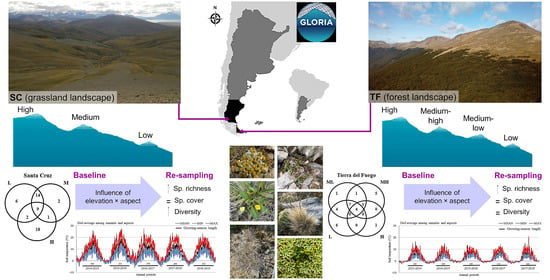
33]. However, there is a lack of information about temporal changes in alpine plants and temperatures at high southern latitudes. Therefore, the objectives of this work were: (1) to evaluate variations in alpine vascular plant diversity between the baseline and first re-sampling after a five-year period, at different topographic (elevations and cardinal aspects) conditions, in mountains located in two contrasting landscapes (foothill grasslands and sub-Antarctic forests) of South Patagonia; (ii) to analyze main variations in soil temperatures and growing-season length over five annual periods following the baseline sampling, relating them to ENSO climatic variations. We hypothesized that (i) alpine plant composition varies with dominant vegetation type of the surrounding landscape (forest or grassland), and richness, cover and diversity indices diminish with elevation gain, expecting even lower values in more exposed cardinal aspects, while changes in time mirror general trends caused by global warming (movement upward of thermophilic plant species, and loss of cryophilic species); (ii) soil temperatures (mean, minimum and maximum) and growing-season length diminish with elevation gain, expecting even lower values in more exposed cardinal aspects, and increase over time because of global warming, although ENSO climatic variations also impact on these variables. At these southern latitudes, the large deficiency of floristic alpine vegetation studies and the lack of evidence about topographical and temporal changes in alpine vegetation and soil temperature dynamics from long-term studies, reinforce the importance of this study.

2. Materials and Methods

2.1. Sampling Sites

The study was developed at two mountainous sites of South Patagonia (Argentina), located in SC (49.767302° SL, 72.521677° WL) and TF (54.660648° SL, 67.760100° WL), as part of the international GLORIA Multi-Summit Approach (www.gloria.ac.at, accessed 30 May 2021), and PEBANPA network (Biodiversity and Ecological long-term plots in southern Patagonia [34]).
In SC, the GLORIA Approach includes three different summits in the foothill of the Andes mountains, belonging to a sub-alpine grassland ecological area [35]. The three summits share a similar general climate and reach the following maximum elevations: 814 m a.s.l. or low (L); 887 m a.s.l. or medium (M); and 1085 m a.s.l. or high (H). These correspond approximately from sub-alpine to sub-nival habitats. According to the classification of Köppen-Geiger [36], the climate type in this area is BWk (cold arid desert), with a mean annual temperature of 6 °C, a mean temperature in the warmest month (January) of 10 °C, and a mean temperature in the coldest month (June) of 3 °C. The prevailing winds blow westerly, and rainfall reaches 1750 mm per year [37]. The sub-alpine grassland is mainly dominated by grasses, e.g., Festuca pallescens, F. argentina, and Pappostipa chrysophylla var. chrysophylla, and shrubs, e.g., Azorella prolifera, Berberis microphylla, and Mulguraea tridens [35]. Extensive livestock breeding (sheep) occurs at this site, with variable stocking rates ranging from 0.13 to 0.75 head ha−1.year−1 [24].
In TF, the mountain pilot site includes four summits in a single mountain chain of the Fuegian Andes, belonging to the sub-Antarctic forest ecological area [29]. The four summits share a similar general climate and reach the following maximum elevations: 634 m a.s.l. or low (L); 673 m a.s.l. or medium-low (ML); 782 m a.s.l. or medium-high (MH); and 864 m a.s.l. or high (H). These correspond approximately from sub-alpine to nival habitats. According to the classification of Köppen-Geiger [36], the climate type in this area is ET (tundra), with a mean annual temperature of 2 °C, a mean temperature in the warmest month (January) of 3 °C, and no months with mean temperatures below freezing (1 °C in June, the coldest month). Summers are short and cold, and winters are long, snowy, and with long freezing spells. The prevailing winds blow south-westerly, and rainfall reaches 545 mm per year [37]. The forest is dominated by the deciduous Nothofagus pumilio tree, mixed in some patches at mid-slope with the perennial N. betuloides. Treeline is the same for both species (approximately 600 m a.s.l.), growing with a scrubby habitat. The understory is scarce, with few forbs (e.g., Osmorhiza depauperata, Senecio acanthifolius), ferns (e.g., Blechnum penna-marina, Cystopteris fragilis), and grasses (e.g., Phleum alpinum, Trisetum cernuum) [29]. No timber is currently extracted from the area, although harvesting was applied between 1950 and 1970 in the low-medium slopes of this mountain chain [38].
The alpine vegetation in the sub-alpine, sub-nival, and nival habitats, both in SC and TF, is mainly dominated by dwarf shrubs (e.g., Nassauvia spp., Senecio spp.) and cushion plants (e.g., Azorella spp.) that decrease in abundance with elevation. In addition, there are some forbs (e.g., Perezia spp.) and grasses (e.g., Festuca spp., Poa spp.), but in the highest grasslands, the abundance of vegetation decreases sharply and is replaced by lichens [27,29]. The native fauna consists of birds, rodents, insects, and the large herbivorous mammal Lama guanicoe, that browses freely across the study areas.

2.2. Sampling Methodology

We sampled alpine vascular plants at the species level, following the protocol defined by GLORIA [3]. In the present study, we analyzed from the four 1 × 1 m quadrats located in the 3 × 3 m grid, placed at the four cardinal aspects (north, east, south, and west) of each summit, with the lower boundary of each quadrat cluster lying at the 5 m contour line below the summit. We chose quadrat data due to stronger comparisons in time and with soil temperatures. We sampled across N = 7 × 4 × 4 = 112 quadrats. We performed baseline sampling (BL) in 2013 in TF, and in 2014 in SC. According to the protocol, we re-sampled (RS) each quadrant at each cardinal aspect of each summit, five years later (2018 in TF and 2019 in SC). We registered all plant species, and visually estimated species cover (%) in each quadrat. For species identification, we followed [27] for SC and [29] for TF, and for specific and subspecific epithet, elevation range (m a.s.l.), origin (native or exotic), and endemism identification we followed [39]. We considered endemic species as those only inhabiting South Patagonia provinces in Argentina (SC and/or TF) and/or the two southern regions of Chile (Aysén and/or Magallanes). We deposited voucher specimens of each plant species in the Herbarium of Tierra del Fuego at the Centro Austral de Investigaciones Científicas (CADIC CONICET) in Ushuaia, Argentina. The complete list of vascular plant species is shown in Appendix A.
In the center of the 3 × 3 m grid (n = 12 in SC and n = 16 in TF), we placed temperature loggers (Hobo Pendant, UA-001–64, ONSET, Bourne, MA, USA) to register hourly soil temperature (±0.1 °C) at 10 cm depth. Data were continuously registered from 2013 to 2019 and downloaded during February-March each year. There are some gaps in the dataset due to equipment failure. In event of failure, loggers were replaced, or removed and reinstalled 1–2 days later. Those gaps in data were completed with extrapolation and short modelings.
We also characterized climatic variations produced by ENSO events, through Multivariate ENSO Index version 2 (MEI). MEI was obtained for the studied period (2013–2014 to 2018–2019) from the NOAA Physical Science Laboratory (data available at http://www.esrl.noaa.gov/psd/enso/mei/, accessed 12 June 2021). It was calculated for 12 overlapping bi-monthly “seasons” (December–January, January–February, February–March, …, November–December) to consider ENSO’s seasonality, and to reduce the effects of intra-seasonal variability [40]. MEI indicates the occurrence of El Niño conditions when the index is positive (>0.5), La Niña conditions when it is negative (<−0.5), and normal conditions when it is in between [40].

2.3. Data and Statistical Analyses

We determined species richness (number of species), cover (%), and occurrence frequency (%) for the entire study, each summit, and each sampling date. We analyzed species composition particularities (including shared and exclusive species), elevation range, origin, and endemism, comparing SC and TF to analyze the influence of dominant vegetation in the surrounding landscape (grasslands and forests).
We then determined species richness, cover, Shannon–Wiener diversity (SW), and Pielou evenness (J) indices [41] for alpine vascular plant diversity in each quadrat. We analyzed differences in their average values by performing three-way ANOVAs, considering summit elevation (A), cardinal aspect (B), and sampling date (C) as the three main factors that contribute to the evaluation of the first hypotheses. We first verified normality and homoscedasticity assumptions for each variable and applied Tukey tests (p < 0.05) for mean comparisons. We also evaluated interaction terms among the three main analyzed factors (A × B, A × C, B × C, and A × B × C). We plotted significant interactions and analyzed them by one-way ANOVA, comparing means by the Tukey test (p < 0.05).
In addition, three multivariate statistical analyses were performed based on a matrix of species cover: (i) non-metrical multidimensional scaling (NMS), using Bray-Curtis distance and 500 iterations, to graphically represent similarities in the assemblage composition of plots according to elevation and aspect, and species association; (ii) multi-response permutation procedures (MRPP), also with Bray–Curtis distance, to test differences in composition among groups defined by the levels of the main factors (elevation, aspect, and sampling date); and (iii) indicator species analysis (IndVal) [42], to explore possible associations between vascular plants and summits, aspects or sampling dates. Both analyses were performed for SC and TF separately and complemented the ANOVAs to analyze the first proposed hypothesis.
In the NMS, three components were generated, for which significance was evaluated with a Monte Carlo permutation test (500 randomizations). Graph rotation was applied when needed for better representation. In the NMS for SC data, N and W plots of the highest summit were excluded from the analysis, because these had just two species that only occurred in these plots, generating an exaggerated influence on the ordering. In the MRPP, we evaluated the statistic (T), the associated probability (p), and the chance-corrected within-group agreement (A) [43]. Subsequent pairwise groupings were tested to determine the significance of the differences (p < 0.05) [44]. For IndVal, we considered indicator species as those with an indicator value > 0.40 and p < 0.05.
Soil temperature (°C) data were analyzed for the five annual periods between baseline and re-sampling: 2014–2015 to 2018–2019 in SC, and 2013–2014 to 2017–2018 in TF. As each new year starts in the middle of the growing season in the southern hemisphere, we considered each annual period from the beginning of the winter through the end of autumn (21 June to 20 June of the following year). For each elevation and aspect, we estimated the growing-season length considering: (i) the first and last incidence of mean temperatures above +2 °C [45]; and (ii) the continuous recording of these values for 7 or more days to account for the sporadic high climatic variability and extreme weather events in South Patagonia (e.g., short snowstorms in spring, eventual frosts in summer).
To evaluate the second hypothesis, we analyzed monthly mean, and absolute minimum and maximum soil temperatures by three-way ANOVAs, considering summit elevation (A), aspect (B), and annual period (C) as the three main factors. We first verified normality and homoscedasticity assumptions for each variable and applied the Tukey test (p < 0.05) for mean comparisons. We also evaluated interaction terms among the three main analyzed factors (A × B, A × C, B × C, and A × B × C). We plotted significant interactions and analyzed them by one-way ANOVA, comparing means by the Tukey test (p < 0.05). For the growing-season length, we compared homogeneity of values among elevations, aspects, annual periods, and their combination (e.g., elevation and aspect), employing the chi-square test (p < 0.05). Finally, we calculated annual mean, spring-summer, summer and winter MEI for the six studied annual periods and compared these values with soil annual mean temperatures and growing-season lengths at each summit. Statgraphics Centurion XVI was used for all the ANOVAs, chi-square, and related tests; PC-ORD [46] was used for NMS, MRPP, and indicator species analyses.

3. Results

3.1. Plant Variation

The total species richness was higher in SC, with 52 sp., than in TF, with 30 sp. (Appendix A). However, the mean vegetation cover was only half as high in SC (24%) as in TF (50%). We identified 27 plant families (Table 1): 20 in SC and 12 in TF. Among these, we found 15 exclusive families in SC (e.g., Amaryllidaceae, Calceolariaceae, Ephedraceae) and 7 in TF (e.g., Empetraceae, Ericaceae, Thymelaceae), with only 5 families in common. Asteraceae (22 sp.) and Poaceae (16 sp.) were the richest families across the two sites, with 14 sp. and 9 sp. in SC, and 8 sp. and 7 sp. in TF, respectively. No species occurred at both sites (Appendix A), and only two exotic grasses were detected: Dactylis glomerata in SC and Poa pratensis in TF. Endemism was also important at both sites, with 7 sp. in SC and 6 in TF. In relation to species distribution across elevations, 73% of the total richness in SC and 87% in TF were present in wide ranges of elevation (Appendix A), from the sea level (0 m a.s.l.) to medium elevations (1000–2000 m a.s.l.), or from the sea level to high elevations (3000–4300 m a.s.l.). Only 9 sp. in SC and 3 sp. in TF occurred at elevations higher than 500 m a.s.l.
Total richness and mean vegetation cover decreased with elevation gain in TF (from 21 to 6 sp.; and from 95% to 9% cover) (Table 1). This was not the case in SC (31 sp. in L, 26 in M, and 30 in H), where mean vegetation cover was similar at L and M (31–34%) and lower at H (6%). In addition, there were few shared species among all summits within each site (9 in SC and 4 in TF), contrasting with species exclusively found on each summit (Figure 1). Exclusive species varied from 18 sp. in H to 2 in M in SC, and from 6 sp. in L to 1 in ML and H in TF. Moreover, L and M in SC contained the highest amount of species shared between two summits (14 sp.).
With regards to temporal changes, 40 sp. in SC and 23 in TF were observed on both sampling dates. Four sp. in SC and 1 in TF were only found in the baseline, while 8 sp. in SC and 6 in TF were new in the re-sampling (Appendix A). In SC, species loss occurred at L (D. glomerata and Rytidosperma virescens) and H (Azorella sp. and an undetermined Asteraceae), while in TF, only 1 (P. alpinum) disappeared over time in L. In addition, in SC, we recorded 5 new sp. at H (Nassauvia sp., Perezia pilifera, Trisetum subsp. cumingii, Valeriana moyanoi, and V. sedifolia), 4 at L (Bromus catharticus, Calandrinia caespitosa, Hypochaeris incana, and T. subsp. cumingii) and 1 at M (V. moyanoi). While in TF, the highest appearance of new species in re-sampling occurred in MH (Deschampsia parvula, Gamochaeta spiciformis, Nassauvia pygmaea, P. pratensis, and an undetermined species), compared with only 1 new species at ML (D. parvula) and at L (Azorella ranunculus). The movement of plant species across summits was also recorded. In SC: Alstroemeria patagonica moved upward from L in the baseline to M in the re-sampling; Poa secunda occurred at L and M on both sampling dates, but also had moved upward (H) in the re-sampling; Olsynium biflorum and Vicia magellanica were recorded at L and M in the baseline, but only at M during the re-sampling. In TF: Senecio humifusus was observed at ML, MH, and H in the baseline, but it was missing at H in the re-sampling; Poa alopecurus ssp. fuegiana occurred at L, ML, and MH in the baseline, but only at higher elevations (ML and MH) when re-sampled (Appendix A).
Significant differences (F > 2.09; p < 0.04) were found for all variables (mean richness, vegetation cover and diversity indices) according to elevation, aspect and sampling date in SC and TF (Table 2). Interactions occurred between elevation and aspect, for all variables, on both sites (F > 3.26; p < 0.01), showing different responses at different summits depending on the aspects (Figure 2). In SC, significant interaction between elevation and sampling date occurred for evenness index (F = 3.82; p = 0.03), and a three-factorial interaction was detected for vegetation cover (F = 3.26; p = 0.01). Other interactions were not significant for all variables on both sites (F < 2.59; p > 0.06).
In SC, elevation × aspect interactions were mainly explained by very low values in N and W aspects (less than 1 sp. per m2, 0.1% cover, 0.17 SW, and 0.24 J) on the highest summit, when compared with E and S (more than 10 sp. per m2, 7.5% cover, 1.50 SW and 0.65 J). L showed the highest values in richness, diversity, and evenness indices on E (9.4 sp., 1.55 SW, and 0.69 J), and the lowest values on the N aspect (5.6 sp., 0.59 SW, and 0.34 J), while the cover was the greatest on W (46%) and the barest on S (18%). At M, the highest and lowest values occurred in different patterns for all variables, with the highest richness and diversity found on the W aspect (13.4 sp. and 1.50 SW), cover on E (58%), and evenness on S (0.62 J). Minimum values were recorded on N aspect for richness and cover (6.9 sp. and 14% cover), and E for diversity and evenness indices (0.45 SW and 0.23 J).
In SC, the interaction between the summit and sampling date for evenness index occurred because values decrease with elevation gain in the baseline (from 0.55 to 0.42 J), but similar values were observed for the three summits in re-sampling (0.57, 0.53, and 0.61 J for L, M, and H, respectively). However, significant differences were not detected among evenness values (F = 1.18; p = 0.33). Concerning the three-factorial interaction showed that while cover in baseline and re-sampling had similar values in differing aspects and summits (mainly in H), cover values varied greatly among aspects depending on the elevation. Thus, N, W, and S aspects at H exhibited the lowest cover values (less than 3% on average); E at H, as well as N at M, and S at L had medium-low cover values (16% on average); W and S at M and E and N at L showed medium-high cover values (31% on average), and Eat M and W at L exhibit the greatest cover values (from 45% to 68% on average). Complementary, significant differences were found between sampling dates for richness and diversity index in SC (F > 4.28; p < 0.04), with greater values in the re-sampling than in the baseline for both variables (Table 2).
In TF, elevation × aspect interactions in richness and cover were mainly explained by similarly low values across all aspects at H (1.2 sp. per m2 and 9% cover in average) compared with the other summits (6.6 sp. and 63% cover on average), while different trends among aspects were observed at the other three elevations (Figure 2). For example, while at L richness showed the highest values on W (12.9 sp.) and the lowest on N and E (6.2 sp. on average), the highest richness was observed at ML on N and S aspects (8.8 sp. on average) and the lowest at E (2.9 sp.). Concerning cover, L displayed similarly high values on all aspects (95% on average); while ML showed the greatest cover on S (88%). On the other hand, maximum and minimum SW and J occurred on different aspects at each summit, for which the highest values were detected on the W aspect for L and ML (1.1 SW and 0.5 J, on average for the two summits), on N aspect at MH (1.2 SW and 0.6 J), and on S at H (0.5 SW and 0.6 J); and the lowest on E aspect at L and ML (<0.1 SW and J, on average for the two summits), on S at MH (0.1 SW and <0.1 J), and on W and N at H (<0.1 SW and J). Besides this, re-sampling in TF exhibited the highest richness but the lowest evenness (F > 4.85; p < 0.01).
Analysis of plant species assemblage patterns by NMS (Figure 3) showed plots joined in three groups, at both sites. In SC, where a bi-dimensional solution was recommended (p < 0.01 for Axis 1 and p < 0.01 for Axis 2; 8.029 final stress; 0.034 final instability), one group was made up of H plots, associated with several exclusive species (e.g., Moschopis trilobata). Another group was made up of E-facing plots at L and M, associated with common grasses, forbs, and shrubs of the lowland sub-alpine grassland, including F. pallescens, V. magellanica, and A. prolifera, and the only one exotic grass in SC, D. glomerata. The third group occurred by similar composition among N, S, and W facing plots at L and M, related to some grasses (e.g., P. chrysophylla var. chrysophylla), woody dwarf shrubs (e.g., Ephedra chilensis), and cushion plants (e.g., Nassauvia glomerulosa). MRPP highlighted the assemblage differences among elevations and aspects in SC (Table 3), showing significant differences among H and the other elevations (p < 0.01), as well as among E and the other aspects (p < 0.01). Significant differences were not detected between L and M elevations (p = 0.07); N, S and W aspects (p > 0.12); nor sampling dates (p = 1.00).
Similarly, three plot groups were distinguished by NMS in TF, where a tri-dimensional solution was recommended (p < 0.01 for Axis 1 and p = 0.01 for Axis 2; 6.049 final stress; 0.061 final instability). S and W facing plots of H formed one group; in the second group, N and E at H, and N, S and W at MH were joined; and in the third group, plots of all aspects at L and ML, plus E plots at MH were closely ordered. The first group was strongly characterized by the presence of Senecio alloeophyllus var. alloeophyllus. The second group was correlated with some forbs (e.g., Acaena antarctica) and the exotic grass P. pratensis. The third group was related to species found across a wide range of elevations, mainly associated with poorly drained soils (e.g., Marsippospermum grandiflorum), and several types of grass (e.g., Festuca contracta), dwarf shrubs (e.g., Empetrum rubrum), and cushions (e.g., Bolax gummifera). MRPP also highlighted differences in assemblage composition in TF, showing significant differences between elevations (p < 0.03) except for L vs. ML (p = 0.18), but similar plant assemblages on all aspects (p > 0.08) and significant differences only for E vs. W (p < 0.01). As was the case in SC, differences in TF plant assemblages were not found between sampling dates (p > 0.99).
Finally, IndVal analyses (Table 4) found indicator species for all elevations, both in Santa Cruz (2 sp. in L, 4 sp. in M, and 7 sp. in H) and TF (4 in L, 2 in ML, 1 in MH and 1 in H). Indicator species were found on three of the four aspects in SC (6 sp. on E; 2 sp. on W and 2 sp. on S), but only on one aspect in TF (1 sp. on E). Similarly, there was 1 sp. defined as an indicator of re-sampling in TF.

3.2. Soil Temperature Variation

Over the five years of this study, average mean and maximum annual soil temperatures reached higher values in SC (5.8 °C and 15 °C in average, respectively) than in TF (2.1 °C and 6.7 °C, respectively). The minimum soil temperature was similar at both sites (−0.3 °C in SC and −0.4 °C in TF). The diel absolute maximum value in the entire study periods was 33.5 °C in SC and 30.6 °C in TF, while the minimum value was −9.5 °C in SC and −7.5 °C in TF (Appendix B).
In SC (Table 5), monthly mean and absolute minimum and maximum soil temperatures significantly decreased with elevation gain (F > 6.53; p < 0.01). The absolute maximum temperature significantly varied between years, showing higher values in 2016–2017 than at the first (2014–2015) and last (2018–2019) periods. Significant differences were not detected among aspects and annual periods in mean and absolute minimum temperatures (F < 2.35; p > 0.05). Interactions were not significant for all variables (F < 1.90; p > 0.08).
In TF (Table 5), monthly mean soil temperature also significantly decreased with elevation gain (F = 11.89; p < 0.01). The absolute minimum and maximum temperature exhibited significant interactions between elevation and aspect (F > 2.07; p < 0.03). In the minima, the interaction was explained by extreme values (the lowest and the highest) at each summit on different aspects: E, W, W, and N aspects showed the lowest values, and W, N, N, and E aspects displayed the highest values, at L, ML, MH and H summits, respectively (Figure 4). This resulted in minimum temperatures above 0 °C on the N aspects of all summits except for the highest one, which had the coldest value. In the maxima, the lowest values occurred on the S aspect in all elevations, but the highest values were observed on E, W, W, and N aspects at L, ML, MH, and H summits, respectively. Consequently, the maximum temperature increased with elevation gain on the N aspect, reaching the warmest value compared with all other aspects and elevations at the highest elevation summit. Temperature increase with elevation gain was not observed in the other aspects. There were no interactions for mean temperature in TF (F < 0.42; p > 0.91), and other interactions were not significant for minimum and maximum temperatures (F < 0.63; p > 0.81).
In relation to the growing season, the diel mean temperature in SC fluctuated between 10 and 20 °C across all elevations and aspects (Appendix B), while in TF, it ranged from 5 to 10 °C, with higher diel fluctuations on higher summits and sunnier aspects (e.g., N at H). On the other hand, the non-growing season was characterized by hardly any diel fluctuation in some years and aspects at both sites (e.g., winter 2015 on S and W at H in SC; all winters and aspects at L in TF). The growing-season length varied more in SC (192 to 323 days) than in TF (117 to 227 days), with more homogeneity among aspects on each summit for SC (p > 0.82) than for TF (p > 0.64). Likewise, the growing-season length on each aspect was more similar among summits in SC (p > 0.52) than in TF (p > 0.08), where W showed greater differences in growing-season length among summits. In addition, N exhibited long growing-season on the lowest summits at both sites, while short growing-season lengths were observed on S aspects of the highest summits at both sites. Finally, interannual variations influenced growing-season length both in SC and in TF (e.g., tending to lengthen the growing season during 2015–2016 in TF and 2016–2017 in SC, and to shrink it during 2014–2015 in TF and 2017–2018 in SC).
Concerning ENSO, a La Niña event (1.647 mean annual MEI) occurred in the 2015–2016 period, while 2017–2018 was El Niño (−0.769 mean annual MEI), with other periods showing near normal values (from −0.359 to 0.387 mean annual MEI). These trends were also maintained for mean spring-summer, summer, and winter MEI. Likewise, the La Niña period exhibited high mean annual soil temperatures across all summits in SC (7.0 °C in L to 5.3 °C in H), and at the low elevation in TF (2.6 °C in L to 1.0 °C in H), with reverse trends in El Niño period: low mean annual soil temperatures in SC (6.5 °C in L to 4.4 °C in H) and high mean annual soil temperatures in TF (3.1 °C in L to 1.4 °C in H). Medium mean annual temperature values were reached in normal periods at both sites. Concerning the average growing-season length, the annual period with La Niña event showed in TF the longest growing-season lengths across all summits (209 days at L to 189 days at H), the shortest growing-season lengths (172 days at L to 162 at H) in the annual period with El Niño event, and medium values in normal periods. However, in SC, the longest growing-season lengths occurred in normal years for all summits (270 days at L to 248 days at H), and the shortest growing-season lengths were during El Niño event (253 days at L to 228 days at H), with values between the two extremes during La Niña event.

4. Discussion

The analyzed plant species assemblages, both in SC and TF, were mostly composed of typical lowland species (more than 70% of the total richness in each site) that are naturally widely distributed across a wide range of elevations. For example, Azorella monantha, Chiliotrichum diffusum, and Nassauvia darwinii, occupy broad latitudinal (e.g., from 32° to 54° LS) and altitudinal gradients (e.g., from 0 to 3000 m a.s.l.) [39]. However, these species are smaller in alpine habitats compared with lowlands, as was observed in Chiliotrichum diffusum (>1 m average height in lowlands [29], but <20 cm average height in alpine habitats). On the other hand, only a small proportion (17% of total richness in SC and 10% in TF) were mountain species. The presence of lowland species at high elevations is common poleward, due to similarities between environmental conditions at high elevations and high latitudes, but this has been much more described for arctic regions [3]. On the other hand, several of the observed species (e.g., Adesmia aphanantha, Astragalus palenae, Tristagma nivale, and V. moyanoi) are naturally widely distributed across mountains of the entire Patagonia [39]. However, we only found them in one province (SC or TF); this is likely because plant communities in mountains are locally more heterogeneous and patchier than in lowlands, as these communities can only survive in restricted favorable microsites when the climate becomes less hospitable at higher elevations [47] or latitudes. In summary, assemblages were different between the mountain sites of SC and TF, without any species in common, reflecting differences in the surrounding vegetation and partially confirming our first hypothesis. Differences in species composition between the two sites were also highlighted by exclusive and endemic species, some of which were also identified as indicator species of the studied assemblages, mainly in Tierra del Fuego. The high representation of endemism among the indicator species has also been observed in mountains in other parts of the world (e.g., [10]). However, the lack of knowledge about the vascular alpine plant assemblage composition in other mountainous regions of SC and TF makes it difficult to extrapolate endemic species value as indicator species for the entire region, even at similar elevations and aspects. More studies are needed across mountains to improve knowledge about species specificity and fidelity to a given elevation and aspect in South Patagonia. For example, through this study, 5 species in SC (Acaena platyacantha, Benthamiella spegazziniana, Philippiella patagonica, V. moyanoi, and V. magellanica) and 3 in TF (A. antarctica, S. alloeophyllus var. alloeophyllus, and S. humifusus) were found outside of their expected elevation ranges, as was reported in other GLORIA works [17].
The presence of exotic species in alpine plant assemblages is usually uncommon [48,49], although P. pratensis was also observed in high mountain areas of México [50]. In our study, the presence of exotic species may be related to domestic (e.g., sheep, cows, and horses) and/or native (L. guanicoe) herbivorous mammals that graze freely in the study area, as is often observed in other alpine ecosystems (e.g., [51]). The spread of exotic plants could be facilitated by the increase in accessibility (e.g., [52]). However, the disappearance of D. glomerata in the re-sampling of SC denoted their low capability to survive in alpine conditions. Despite observed differences in the two studied sites, some taxonomic overlapping occurred between them when the species list of the entire summit area (up to 10 m down a level from the top) was compared. For example, Azorella lycopodioides, B. microphylla, and M. grandiflorum were common species in both provinces across the entire summit area (data non-shown), displaying the influence of the sampling method.
The increase in richness and diversity comparing re-sampling to baseline in 1 m2 quadrats, as well as the upward movement of species, both in SC and TF, is consistent with the short-term rise in species richness in other monitoring studies (e.g., [19,53,54,55]). This could be interpreted as an early indicator of climate change-driven warming, despite we did not detect soil warming over the studied five-year period. Also, downslope range shifts may constitute an indirect response to warming caused by changes in species interactions, as well as to habitat modification [56]. Instead of long temporal temperature data series in South Patagonia outside cities, climate change estimations following CSIRO model in B2 scenario predicted for 2080, +3 °C warming in the mean maximum temperature in SC and +2 °C in the north of TF [37]. Drivers of changes in richness and movement of species should be confirmed with more specific studies, such as those performed by [9,18,57], who reported upward mountain movements of more-thermophilic species and downslope shifts caused by warming [56].
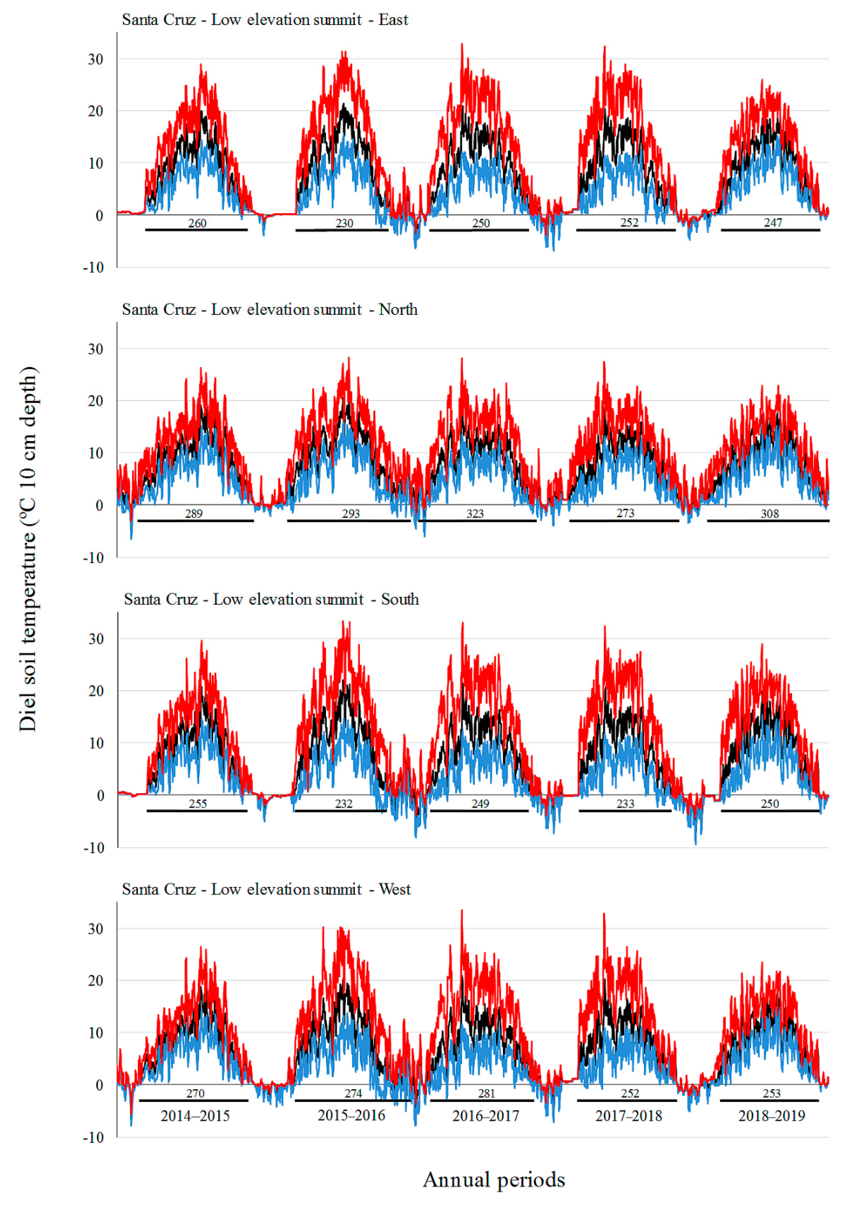
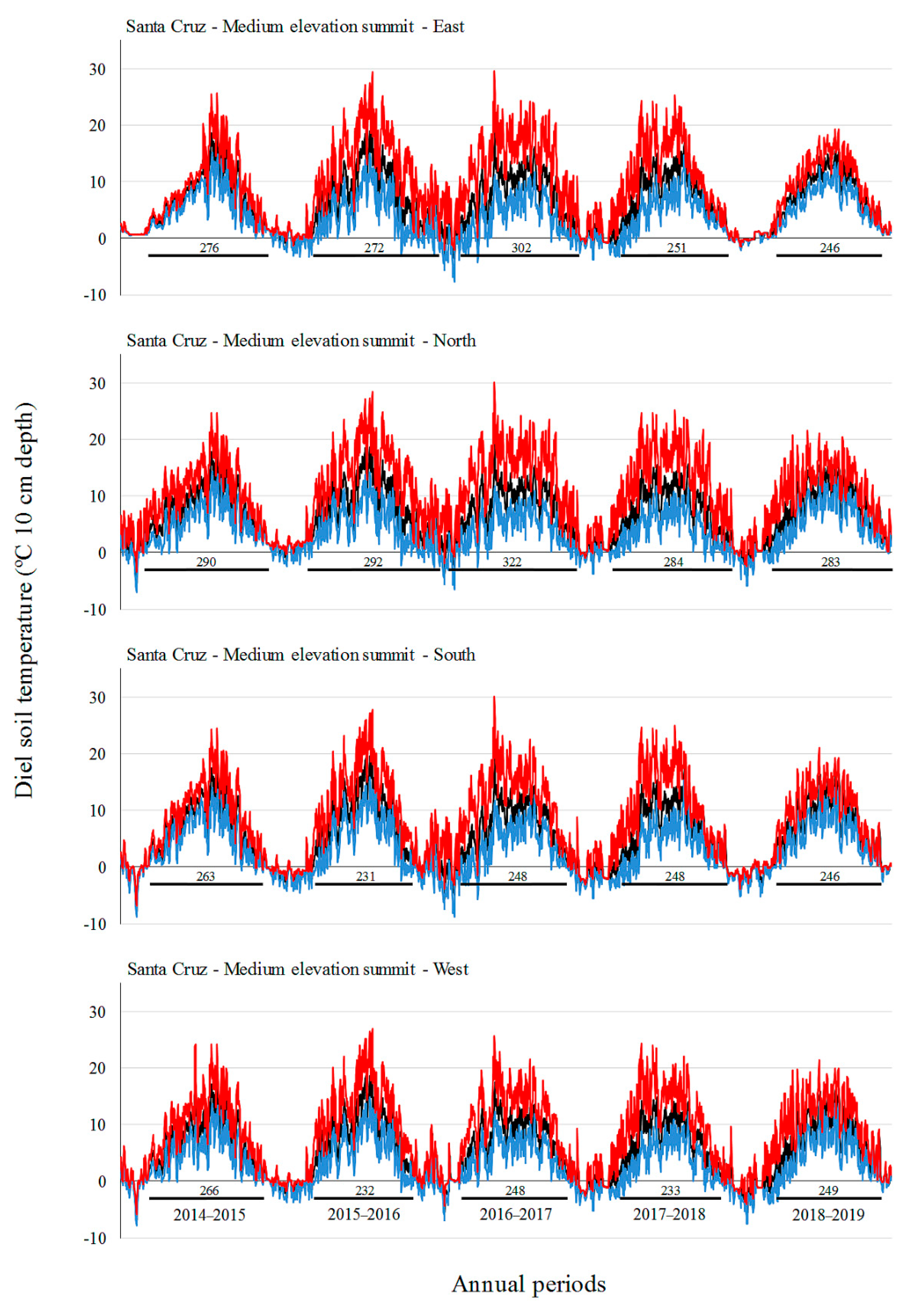
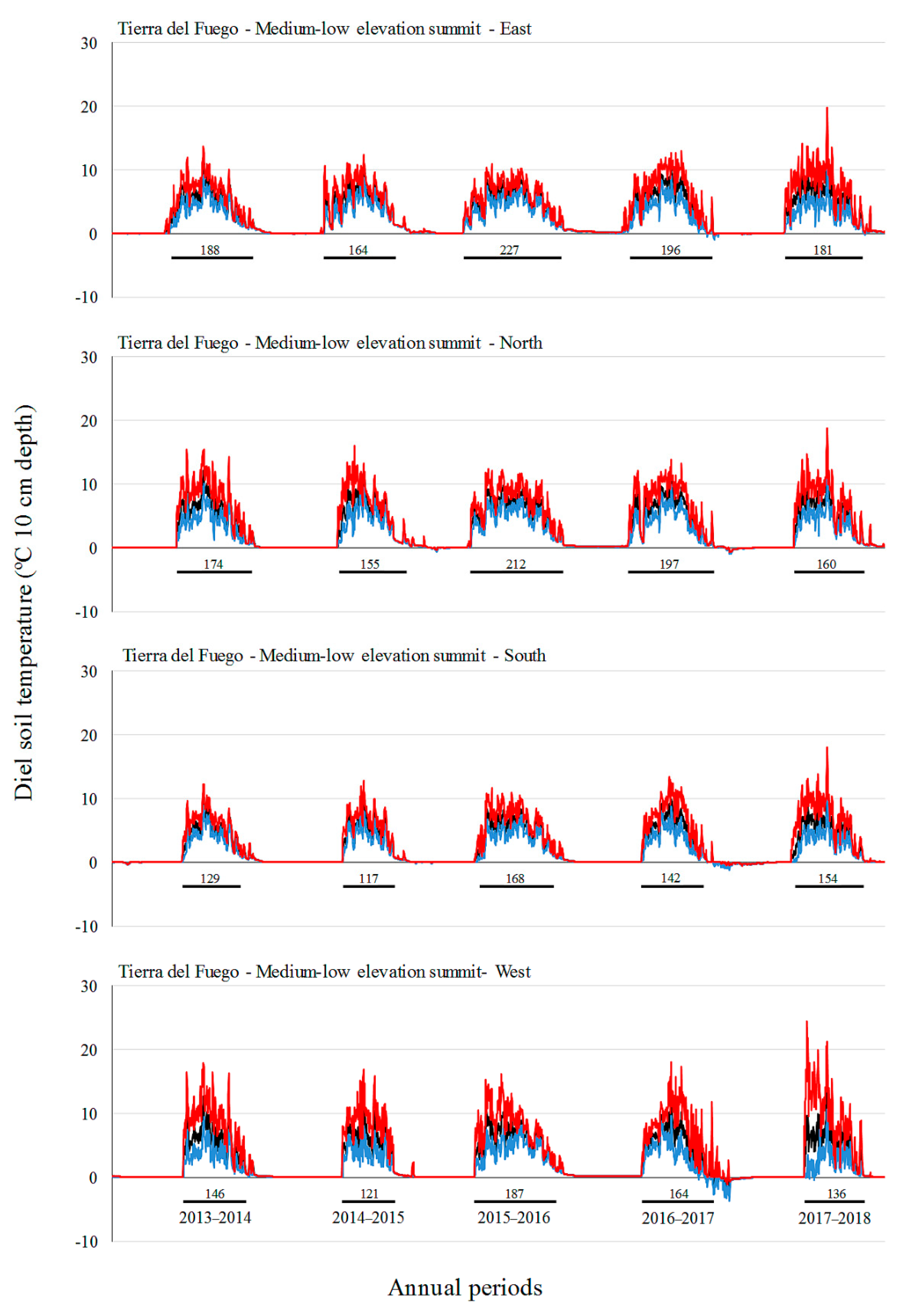
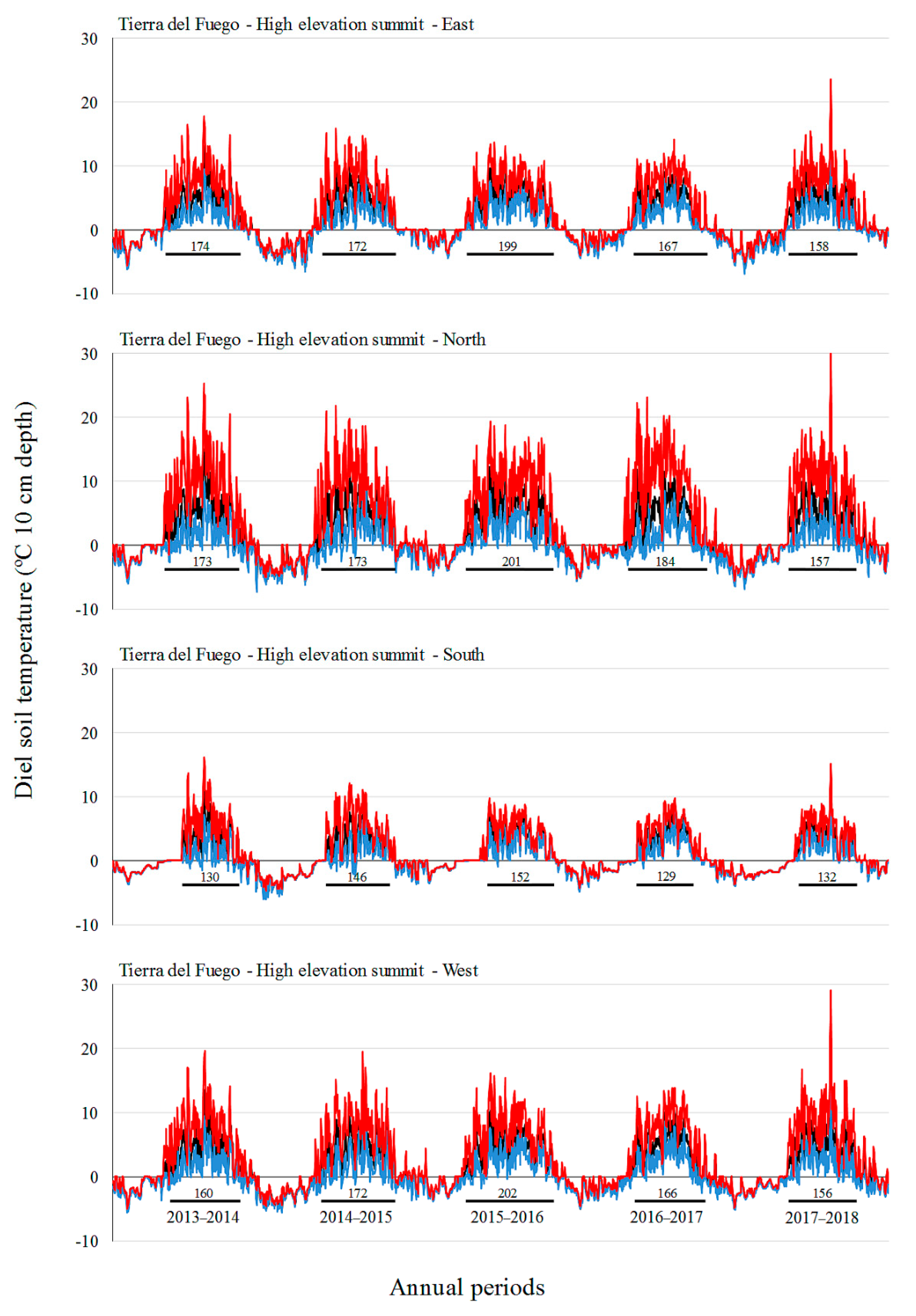
Monthly mean and absolute maximum and minimum temperatures did not increase over time in our study, with the highest values in the middle annual periods (2015–2016 and 2016–2017 for SC, 2016–2017 for TF). In the period 2016–2017, SC showed the longest growing season. Ref. [19] also did not observe a gain in soil temperatures over a seven-year period at a GLORIA pilot site off the southern coast of Australia, but they did find an increase in species richness. These authors argue that the increase in species richness in those Australian alpine areas could be explained by the influence of other environmental factors (e.g., rainfall, microsite availability, species interactions, and dispersal/recruitment potential in the regional species pool) rather than climate warming. The influence of ENSO has already been demonstrated in South American alpine environments [17]. We found contrasting effects of ENSO in soil temperature and growing season in the two sites of the present study, that found inverse trends (e.g., higher soil temperatures in SC, but lower soil temperatures in TF during a La Niña event). How ENSO affects mountain climate in South Patagonia should be studied in greater depth. Additionally, the observed increase in alpine species richness could be a delayed expression of vegetation changes [58], which could start and be sustained by greater warming rates that occurred many years ago (e.g., during the 70s decade), as is commonly observed in lags in tree regeneration advances above established treelines [59]. In this sense, long-term studies in remote places like Patagonia are important to better understand the effect of climate change on plant richness and vegetation cover in alpine areas across the southern hemisphere.
Elevation had an important influence on vegetation and soil temperature in SC and TF, as it was expected based on other mountain studies (e.g., [8,
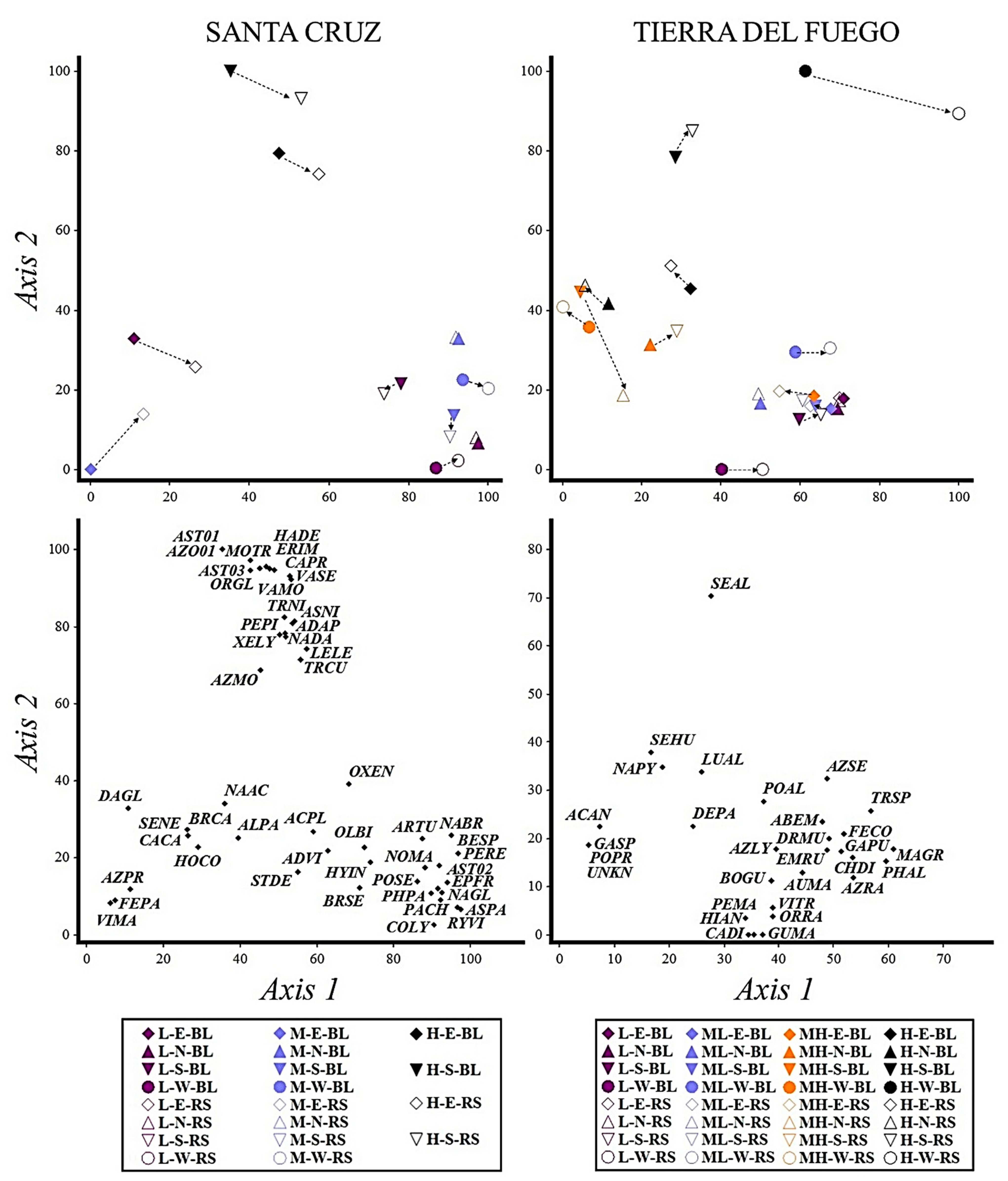
10], richness, cover, and mean temperatures generally decrease with elevation). In contrast to TF, the highest summit of SC contained the highest amount of exclusive species (Figure 1). Species whose distribution was restricted to the highest summit have a particularly strong tolerance for high mountain extreme climatic conditions (e.g., [60,61]), more adaptations to the cold [62], and low competition abilities [63]. It is likely that the continuity of high Andean mountain peaks (>1000 m a.s.l.) favors the colonization of mountain areas in SC, from northern to southern latitudes, by species with particular requirements typically found in the mountains of the central Argentinean Andes (Río Negro and Mendoza provinces) up to 2000 m a.s.l. [39]. Some of these species include A. aphanantha, Astragalus nivicola, and Leucheria leontopodioides. In contrast, the continuity of high mountain peaks is interrupted to the south by a low, hilly area near the Magellan Strait, generating a division between the continent and the high mountain chains of TF (Cordillera Darwin). In addition to the change in direction of the Andes from north-south to west-east direction in TF, this division increases the distance to other alpine islands and disrupts alpine plant species dispersion, as has also been observed in the mountains of central Mexican [50]. Many other species, mentioned as characteristic of and exclusive to high elevation mountains in SC and TF (e.g., Moschopis rosulata, Baccharis nivalis) [39], were not found in our study. This could be due to the restricted dispersal abilities of plants in alpine environments, where there is a high prevalence of barochory [64]. However, other authors have suggested that species present in the upper limit of vegetation are controlled by the availability of safe sites for colonization, survival, and growth among rocky substrate [47]. Concerning soil temperature, the snow cover on the higher summits was highly variable and likely depended on micro-topography (e.g., slopes on the steepest peaks are windswept and snow does not persist very long there even in the winter), as other alpine studies have reported (e.g., [45,65,66,67]).
At lower summits on both sites, plant species composition was highly influenced by the surrounding vegetation. Lowland species, with few specific requirements and a high tolerance for mountain temperatures and soil conditions, were able to expand their distribution to the lower summits at both studied landscapes. These species included F. pallescens in grasslands and A. ranunculus in forests. Other species inhabiting mountains were also common in lowland ecosystems (e.g., xeric steppes, peat bogs), species such as A. prolifera, V. magellanica and Senecio neaei in SC, and Austrolycopodium magellanicum and Gaultheria pumila var. pumila in TF. The species that occurred at all elevations (9 in SC and 4 in TF, Figure 1 and Appendix A), had broad habitat ranges, morphological variability, and latitudinal distributions (e.g., A. monantha, Azorella selago, Nardophyllum bryoides, E. rubrum, Luzula alopecurus), including several dwarf shrubs and cushions with adaptations to survive under different climatic conditions. Regarding soil temperatures, we registered a long series of values around 0 °C in the lowest summits on both sites, due to deep snow cover in wintertime (from May to October) that removes diurnal temperature variations (e.g., [45,65,66,67]).
The cardinal aspect also had a strong influence on vegetation assemblages and length of the growing season both in SC and in TF and was more important than the elevation factor in defining plant assemblages on some summits. This trend was also observed in European mountains by [11,55]. Particularly, northern and western aspects on the highest summit of SC contained only two species (Oxalis loricata and Nassauvia sp.), with very low cover for each (less than 0.1%). The high exposure of these aspects to the cold, dry, and strong (up to 200 km per h) glacial winds, a lack of well-developed soil on very steep slopes, and proximity to icefields (5 km closer than lower summits), reduced plant species establishment and the species pool able to tolerate these conditions. This wind-induced distribution pattern of vegetation in the alpine belt was also observed in the Himalayas [68], where temperatures below 0 °C and the absence of snow protection restricts and limits plant establishment (e.g., on steep slopes).
On the other hand, the significantly different plant assemblages on eastern aspects of the low and medium elevation summits of SC are likely explained by better soil and hydrological conditions, allowing for the growth of species less tolerant to xeric environments (e.g., F. pallescens). Plant species assemblages on eastern aspects were more similar to those of surrounding lowland grasslands exposed to continuous grazing [69]. In contrast, vegetation on north, south, and west-facing plots can be affected by soil erosion and limited water availability for plant growth. This could favor the establishment of prostrated shrubs with taproot systems (e.g., N. bryoides). Conversely, in deeper soils, erosion produces organic matter and nutrient loss in the superficial horizons, generating a sandy texture that favors psamophilic species (e.g., P. chrysophylla var. chrysophylla) [70]. On the other hand, northern slopes were warmer, with earlier snow-melt and longer growing season (Appendix B), probably resulting in earlier vegetation sprouting, and an increased livestock preference for grazing and sleeping when compared to colder and snowier southern aspects [69]. The favorable growing conditions produced by earlier snowmelt and higher summer temperatures on sunnier exposures (south-facing in the northern hemisphere) at low elevations have been documented previously in other alpine habitats across Europe [65] and Asia [45]. Likewise, the significant dominance of xerophilous species, as well as some woody dwarf shrubs (e.g., E. chilensis) and cushion plants (e.g., N. glomerulosa), shows that mountain species in grassland landscapes of South Patagonia are not only associated with temperature but also with water availability, as has been observed in other mountain ecosystems [19,71]. Pits and mounds, as well as rock outcroppings, may also influence soil moisture distribution and stocking. These relationships should be better studied in South Patagonia alpine environments.
In TF, aspect had a stronger influence on vegetation and soil temperature, particularly in high and medium-high elevation summits. Similar to the results obtained in SC, two aspects of the highest elevation summit in TF (southern and western) showed a clear different plant assemblage that had highly reduced richness and cover. The unique species that can survive there (e.g., S. alloeophyllus var. alloeophyllus) are likely those adapted to live on rocks and screes [8]. On the other hand, the species assemblages on north and east-facing plots at the high elevation summit, which were similar to those on northern, southern, and western facing plots at the medium-high summit, consisted of species adapted to receive abundant meltwater or to live in flooded areas (e.g., A. antarctica). Likewise, plant assemblages on the east aspect at medium-high summit exhibited similar composition and cover as those on lower summits. Different aspects on the lower summit showed little variation because of the flat topography, and similar exposure to conditioning factors. In addition, the highest maximum and the lowest minimum temperature in the northern aspect of the highest summit can be explained by the fact that these areas are always free of snow, even during the coldest months, because of their exposure to strong winds. These winds cause winter temperatures to drop very low, while during the growing season they become warmer than other aspects, due to strong insolation [45]. Although temperatures in the favorable growth period are important, a thermal condition in the unfavorable period and days with freezing temperatures are significant as well [66]. Additional studies are required to better understand temperature-related limitations in South Patagonia.

5. Conclusions

This work contributes to the understanding of temporal variations in alpine vegetation and soil temperatures as they relate to topography factors like elevation and cardinal aspects in a predominantly oceanic region. Results suggest that factors other than warming (e.g., surrounding landscape features and ENSO) influence vegetation diversity and temperature variations. Deeper knowledge about the effect of climate change on the southern extreme of the South American continent should have great value to our collective understanding of climate change’s effects on both hemispheres. However, more studies are needed to determine the geographic distribution, population dynamics, and dispersal of high elevation alpine plant species, and to clarify the relation between soil temperature and growing-season length variations, thermal niches of the species, and magnitude of temperature changes in the mountains of South Patagonia.

Author Contributions

Conceptualization, M.V.L., P.L.P. and G.J.M.P.; methodology, M.V.L., R.S., J.M.C. and G.J.M.P.; acquisition of data, M.V.L., R.S., J.M.C., H.B., M.P.F., L.M., G.J.M.P. and P.L.P.; formal analysis, M.V.L., R.S., J.M.C.; data curation, M.V.L., R.S., J.M.C.; writing—original draft preparation, M.V.L.; writing—review and editing, M.V.L., R.S., J.M.C., H.B., M.P.F., L.M., G.J.M.P. and P.L.P.; visualization, M.V.L., R.S. and J.M.C.; supervision, M.V.L., P.L.P. and G.J.M.P.; project administration, M.V.L. and P.L.P.; funding acquisition, M.V.L., G.J.M.P. and P.L.P. All authors have read and agreed to the published version of the manuscript.

Funding

This work was conducted with funds provided by PICT2012–1028 and PICT2016–1968, both from ANPCyT-Argentina and from the binational program BMWF-MINCyT 2013–2015.

Institutional Review Board Statement

Not applicable.

Informed Consent Statement

Not applicable.

Data Availability Statement

The datasets are available from the corresponding author on reasonable request.

Acknowledgments

We would like to thank Stefan Schindler, Sabine Rumpf, Leonardo Huertas, Ayelén Alberti, Francisco Mattenet, Horacio Ivancich, John Henn, and other volunteers for their help in the field fieldwork and downloading data loggers. We also thank Matthew Ruggirello for his helpful comments to improve the English language. MVL, GMP, RS, MPF, and JMC acknowledge logistical support by the Ministry of Science and Technology of Tierra del Fuego during re-sampling in 2018.

Conflicts of Interest

The authors declare no conflict of interest.

Appendix A

Table A1. Occurrence frequency (%) of alpine vascular plant species in summits (L = low, M = medium, ML = medium-low, MH = medium-high, H = high) of South Patagonian sites, immersed in grassland (SC = Santa Cruz), or forest (TF = Tierra del Fuego). Data are differentiated by base line (BL) or re-sampling (RS). Life-form (LF) as S = shrub, SS = sub-shrub, EH = erect herb, PH = prostrate herb, CG = caespitose grass, RG = rhizomatous grass, CU = cushions, F = fern), origin as N = native, NE = native endemic of South Patagonia and/or southern regions of Chile; E = exotic, and elevation range (m a.s.l.), are also provided. Species are ordered alphabetically by Family.
FamilySpeciesCodeLFOriginElevationL-SCM-SCH-SCL-TFML-TFMH-TFH-TF
(m a.s.l.)BLRSBLRSBLRSBLRSBLRSBLRSBLRS
AlstroemeriaceaeAlstroemeria patagonica Phil. 1896ALPAEHN0–130019 31
AmaryllidaceaeTristagma nivale Poepp. 1833TRNIEHN300–3200 3844
ApiaceaeAzorella 01AZO01CUN- 6
ApiaceaeAzorella lycopodioides Gaudich. 1825AZLYCUN0–2500 253838381313
ApiaceaeAzorella monantha Clos 1848AZMOCUN0–3000192525255050
ApiaceaeAzorella prolifera (Cav.) G.M. Plunkett & A.N. Nicolas 2017AZPRSN0–1500 66
ApiaceaeAzorella ranunculus d’Urv. 1826AZRAPHN0–900 56
ApiaceaeAzorella selago Hook. f. 1847AZSECUN0–1000 2561931251966
ApiaceaeBolax gummifera (Lam.) Spreng. 1818BOGUCUNE0–3500 889475751919
AsteraceaeAbrotanella emarginata (Gaudich.) Cass. 1825ABEMCUNE0–1000 697569815044
AsteraceaeAsteraceae 01AST01EHN- 13
AsteraceaeAsteraceae 02AST02EHN-13444450
AsteraceaeAsteraceae 03AST03EHN- 3119
AsteraceaeChiliotrichum diffusum (G. Forst.) Kuntze 1898CHDISN0–2700 66
AsteraceaeErigeron imbricatus Vierh. 1916ERIMEHN0–1000 1925
AsteraceaeGamochaeta spiciformis (Sch. Bip.) Cabrera 1961GASPEHN200–1500 6
AsteraceaeHieracium antarcticum d’Urv. 1826HIANEHN0–2000 25256196
AsteraceaeHypochaeris incana (Hook. & Arn.) Macloskie var. incana 1906HYINEHN0–1500 6
AsteraceaeLeucheria leontopodioides (Kuntze) K. Schum. 1900LELEEHN0–1500 619
AsteraceaeNardophyllum bryoides (Lam.) Cabrera 1954NABRCUN0–120062550504419
AsteraceaeNassauvia 01NAS01PHN- 13
AsteraceaeNassauvia aculeata (Less.) Poepp. & Endl. var. azorelloides (Speg.) Cabrera 1982NAACPHN0–1000505025254431
AsteraceaeNassauvia darwinii (Hook. & Arn.) O. Hoffm. & Dusén 1901NADASSN0–1000 1338
AsteraceaeNassauvia glomerulosa (Lag. ex Lindl.) D. Don 1832NAGLCUN0–150075818881
AsteraceaeNassauvia pygmaea (Cass.) Hook. f. var. pygmaea 1847NAPYEHN0–1000 6
AsteraceaePerezia magellanica (L. f.) Lag. 1811PEMAEHN200–1400 2525
AsteraceaePerezia pilifera (D. Don) Hook. & Arn. 1835PEPIPHN0–4300 13
AsteraceaePerezia recurvata (Vahl) Less. 1830PEREEHN0–10003131312566
AsteraceaeSenecio alloeophyllus O. Hoffm. var. alloeophyllus 1971SEALEHNE1300–1800 3169
AsteraceaeSenecio humifusus (Hook. f.) Cabrera 1969SEHUEHNE900–1000 66505019
AsteraceaeSenecio neaei DC. 1838SENESN0–260038381325316
BrassicaceaeNoccaea magellanica (Comm. ex Poir.) Holub 1998NOMAEHN0–40006135044631
BrassicaceaeXerodraba lycopodioides (Speg.) Skottsb. 1916XELYCUNE0–1400 66
CalceolariaceaeCalceolaria polyrrhiza Cav. 1799CAPOEHN500–2000 136
CalyceraceaeMoschopis trilobata Dusén 1907MOTREHNE500–1500 3813
CaryophyllaceaeColobanthus lycopodioides Griseb. 1854COLYCUN0–230031251325
CaryophyllaceaePhilippiella patagonica Speg. 1897PHPACUN0–500 63844
CaryophyllaceaeStellaria debilis d’Urv. 1825STDEPHN0–350013253131
EmpetraceaeEmpetrum rubrum Vahl ex Willd. 1806EMRUSSN0–2800 100100757563693131
EphedraceaeEphedra chilensis C. Presl 1845EPCHCUN0–420019252525
EricaceaeGaultheria pumila (L. f.) D.J. Middleton var. pumila 1990GAPUSSN0–1000 9410075753131
FabaceaeAdesmia aphanantha Speg. 1902ADAPPHN200–1500 2531
FabaceaeAdesmia villosa Hook. f. 1845ADVIPHN0–24006315031
FabaceaeAstragalus nivicola Gómez-Sosa 1977ASNIPHN1000–2000 638
FabaceaeAstragalus palenae (Phil.) Reiche 1897ASPAPHN500–20003113
FabaceaeVicia magellanica Hook. f. 1846VIMAPHN0–50013 1913
GunneraceaeGunnera magellanica Lam. 1789GUMAPHN0–1800 66
IridaceaeOlsynium biflorum (Thunb.) Goldblatt 1990OLBIEHNE0–100025 256
JuncaceaeMarsippospermum grandiflorum L. f.) Hook. f. 1843MAGRCGN0–1000 1919
JuncaceaeLuzula alopecurus Desv. 1808LUALCGN0–1600 13253844312566
LycopodiaceaeAustrolycopodium magellanicum (P. Beauv.) Holub 1991AUMAFN0–1600 31315656
MontiaceaeCalandrinia caespitosa Gillies ex Arn. 1831CACAEHN300–4000 6
OxalidaceaeOxalis enneaphylla Cav.1799OXENEHN0–26001313 256
OxalidaceaeOxalis loricata Dusén 1901OXLOEHNE0–1500 3125
PoaceaeBromus catharticus Vahl 1791BRCACGN0–1000 13
PoaceaeBromus setifolius J. Presl var. setifolius 1830BRSECGN0–50069696338196
PoaceaeDactylis glomerata L. 1753DAGLCGE0–20006
PoaceaeDeschampsia parvula (Hook. f.) E. Desv. 1854DEPACGNE0–1100 38 19
PoaceaeFestuca contracta Kirk 1895FECOCGN200–1100 7588566931311313
PoaceaeFestuca pallescens (St.-Yves) Parodi 1953FEPACGN0–180025252531
PoaceaeHordeum comosum J. Presl 1830HOCOCGN0–4300383166
PoaceaeOrtachne rariflora (Hook. f.) Hughes 1923ORRACGN0–1300 56505038
PoaceaePappostipa chrysophylla E. Desv.) Romasch. var. chrysophylla 2008PACHCGN500–430013503150
PoaceaePhleum alpinum L. 1753PHALCGN0–500 6
PoaceaePoa alopecurus (Gaudich. ex Mirb.) Kunth subsp. fuegiana (Hook. f.) D.M. Moore & Dogg. 1976POALCGN0–1300 6 31382525
PoaceaePoa pratensis L. 1753POPRRGE0–3800 6
PoaceaePoa secunda J. Presl 1830POSECGNE0–60094698188 50
PoaceaeRytidosperma virescens (E. Desv.) Nicora 1973RYVICGN0–34006
PoaceaeTrisetum (L.) K. Richt. subsp. cumingii (Nees ex Steud.) Finot 1890TRCUCGN0–1100 13 6
PoaceaeTrisetum spicatum (L.) K. Richt. subsp. spicatum 1890TRSPCGN0–4700 6631338
RanunculaceaeCaltha dioneifolia Hook. f. 1843CADICUNE0–1100 1313
RanunculaceaeHamadryas delfinii Phil. ex Reiche 1984HADEEHN0–1100 1325
RosaceaeAcaena antarctica Hook. f. 1846ACANPHN1000–1600 1919
RosaceaeAcaena platyacantha Speg. 1897ACPLPHN900–200038503844
RubiaceaeOreopolus glacialis (Poepp.) Ricardi 1963ORGLCUN300–3500 3819
SchoepfiaceaeArjona tuberosa Cav. var. tuberosa 1799ARTUEHN0–150061363751919
SolanaceaeBenthamiella spegazziniana A. Soriano 1948BESPCUNE1000–1500 3844
ThymelaceaeDrapetes muscosus Lam. 1792DRMUCUN0–1000 69813838256
ValerianaceaeValeriana moyanoi Speg. 1897VAMOEHN1000–2500 19 25
ValerianaceaeValeriana sedifolia d’Urv. 1825VASECUNE500–1500 6
ViolaceaeViola tridentata Sm. 1819VITRPHN0–1000 38441919
UnknownUnknown 01UNKNCUN- 13

Appendix B

Figure A1. Diel soil temperature (°C) variation at 10 cm depth during the five studied annual periods (2014–2015 to 2018–2019) on low elevation summit in Santa Cruz, showing separately different cardinal aspects (east, north, south, west). The length of the growing season is also indicated with horizontal black bars (numbers represent days). Black = mean temperature; blue = minimum temperature, and red = maximum temperature.
Diversity 13 00310 g0a1
Figure A2. Diel soil temperature (°C) variation at 10 cm depth during the five studied annual periods (2014–2015 to 2018–2019) on medium elevation summit in Santa Cruz, showing separately different cardinal aspects (east, north, south, west). The length of the growing season is also indicated with horizontal black bars (numbers represent days). Black = mean temperature; blue = minimum temperature, and red = maximum temperature.
Diversity 13 00310 g0a2
Figure A3. Diel soil temperature (°C) variation at 10 cm depth during the five studied annual periods (2014–2015 to 2018–2019) on high elevation summit in Santa Cruz, showing separately different cardinal aspects (east, north, south, west). The length of the growing season is also indicated with horizontal black bars (numbers represent days). Black = mean temperature; blue = minimum temperature, and red = maximum temperature.
Diversity 13 00310 g0a3
Figure A4. Diel soil temperature (°C) variation at 10 cm depth during the five studied annual periods (2013–2014 to 2017–2018) on low elevation summit in Tierra del Fuego, showing separately different cardinal aspects (east, north, south, west). The length of the growing season is also indicated with horizontal black bars (numbers represent days). Black = mean temperature; blue = minimum temperature, and red = maximum temperature.
Diversity 13 00310 g0a4
Figure A5. Diel soil temperature (°C) variation at 10 cm depth during the five studied annual periods (2013–2014 to 2017–2018) on medium-low elevation summit in Tierra del Fuego, showing separately different cardinal aspects (east, north, south, west). The length of the growing season is also indicated with horizontal black bars (numbers represent days). Black = mean temperature; blue = minimum temperature, and red = maximum temperature.
Diversity 13 00310 g0a5
Figure A6. Diel soil temperature (°C) variation at 10 cm depth during the five studied annual periods (2013–2014 to 2017–2018) on medium-high elevation summit in Tierra del Fuego, showing separately different cardinal aspects (east, north, south, west). The length of the growing season is also indicated with horizontal black bars (numbers represent days). Black = mean temperature; blue = minimum temperature, and red = maximum temperature.
Diversity 13 00310 g0a6
Figure A7. Diel soil temperature (°C) variation at 10 cm depth during the five studied annual periods (2013–2014 to 2017–2018) on high elevation summit in Tierra del Fuego, showing separately different cardinal aspects (east, north, south, west). The length of the growing season is also indicated with horizontal black bars (numbers represent days). Black = mean temperature; blue = minimum temperature, and red = maximum temperature.
Diversity 13 00310 g0a7

References

  1. Grytnes, J.A.; Kapfer, J.; Jurasinski, G.; Birks, H.H.; Henriksen, H.; Klanderud, K.; Odland, A.; Ohlson, M.; Wipf, S.; Birks, H.J.B. Identifying the driving factors behind observed elevational range shifts on European mountains. Glob. Ecol. Biogeogr. 2014, 23, 876–884. [Google Scholar] [CrossRef] [Green Version]
  2. Aalto, J.; le Roux, P.C.; Luoto, M. Vegetation Mediates Soil Temperature and Moisture in Arctic-Alpine Environments. Arct. Antarct. Alp. Res. 2013, 45, 429–439. [Google Scholar] [CrossRef] [Green Version]
  3. Pauli, H.; Gottfried, M.; Lamprecht, A.; Niessner, S.; Rumpf, S.; Winkler, M.; Steinbauer, K.; Grabherr, G. The GLORIA Field Manual—Standard Multi-Summit Approach, Supplementary Methods and Extra Approaches, 5th ed.; GLORIA-Coordination, Austrian Academy of Sciences & University of Natural Resources and Life Sciences: Vienna, Austria, 2015. [Google Scholar]
  4. Körner, C. Alpine Plant Life: Functional Plant Ecology of High Mountain Ecosystems, 2nd ed.; Springer: Heidelberg, Germany, 2003. [Google Scholar]
  5. Raupach, M.R.; Finnigan, J.J. The influence of topography on meteorological variables and surface-atmosphere interactions. J. Hydrol. 1997, 190, 182–213. [Google Scholar] [CrossRef]
  6. Löffler, J. Snow cover dynamics, soil moisture variability and vegetation ecology in high mountain catchments of central Norway. Hydrol. Process. 2005, 19, 2385–2405. [Google Scholar] [CrossRef]
  7. Scherrer, D.; Körner, C. Topographically controlled thermal-habitat differentiation buffers alpine plant diversity against climate warming. J. Biogeogr. 2011, 38, 406–416. [Google Scholar] [CrossRef]
  8. Kazakis, G.; Ghosn, D.; Vogiatzakis, I.N.; Papanastasis, V.P. Vascular plant diversity and climate change in the alpine zone of the Lefka Ori, Crete. Biodiv. Conserv. 2007, 16, 1603–1615. [Google Scholar] [CrossRef]
  9. Gottfried, M.; Pauli, H.; Futschik, A.; Akhalkatsi, M.; Barančok, P.; Benito Alonso, J.L.; Coldea, G.; Dick, J.; Erschbamer, B.; Fernández Calzado, M.R.; et al. Continent-wide response of mountain vegetation to climate change. Nat. Clim. Chang. 2012, 2, 111–115. [Google Scholar] [CrossRef]
  10. Salick, J.; Ghimire, S.K.; Fang, Z.; Dema, S.; Konchar, K.M. Himalayan alpine vegetation, climate change and mitigation. J. Ethnobiol. 2014, 34, 276–293. [Google Scholar] [CrossRef] [Green Version]
  11. Winkler, M.; Lamprecht, A.; Steinbauer, K.; Hulber, K.; Theurillat, J.P.; Breiner, F.; Choler, P.; Ertl, S.; Gutierrez Giron, A.; Rossi, G.; et al. The rich sides of mountain summits—A pan-European view on aspect preferences of alpine plants. J. Biogeogr. 2016, 43, 2261–2273. [Google Scholar] [CrossRef]
  12. Chen, I.C.; Hill, J.K.; Ohlemüller, R.; Roy, D.B.; Thomas, C.D. Rapid range shifts of species associated with high levels of climate warming. Science 2011, 333, 1024–1026. [Google Scholar] [CrossRef] [PubMed]
  13. Lenoir, J.; Svenning, J.C. Climate-related range shifts—A global multidimensional synthesis and new research directions. Ecography 2015, 38, 15–28. [Google Scholar] [CrossRef]
  14. Steinbauer, M.J.; Grytnes, J.A.; Jurasinski, G.; Kulonen, A.; Lenoir, J.; Pauli, H.; Rixen, C.; Winkler, M.; Bardy-Durchhalter, M.; Barni, E.; et al. Accelerated increase in plant species richness on mountain summits is linked to warming. Nature 2018, 556, 231–234. [Google Scholar] [CrossRef]
  15. Cuesta, F.; Muriel, P.; Llambí, L.D.; Halloy, S.; Aguirre, N.; Beck, S.; Carilla, J.; Meneses, R.I.; Cuello, S.; Grau, A.; et al. Latitudinal and altitudinal patterns of plant community diversity on mountain summits across the tropical Andes. Ecography 2017, 40, 1381–1394. [Google Scholar] [CrossRef]
  16. Cuesta, F.; Tovar, C.; Llambí, L.D.; Gosling, W.D.; Halloy, S.; Carilla, J.; Muriel, P.; Meneses, R.I.; Beck, S.; Ulloa-Ulloa, C.; et al. Thermal niche traits of high alpine plant species and communities across the tropical Andes and their vulnerability to global warming. J. Biogeogr. 2020, 47, 408–420. [Google Scholar] [CrossRef] [Green Version]
  17. Carilla, J.; Halloy, S.; Cuello, S.; Grau, A.; Malizia, A.; Cuesta, F. Vegetation trends over eleven years on mountain summits in NW Argentina. Ecol. Evol. 2018, 8, 11554–11567. [Google Scholar] [CrossRef] [PubMed]
  18. Fadrique, B.; Báez, S.; Duque, A.; Malizia, A.; Blundo, C.; Carilla, J.; Osinaga-Acosta, O.; Malizia, L.; Silman, M.; Farfán-Ríos, W.; et al. Widespread but heterogeneous responses of Andean forests to climate change. Nature 2018, 564, 207–212. [Google Scholar] [CrossRef] [PubMed]
  19. Venn, S.; Pickering, C.; Green, K. Short-term variation in species richness across an altitudinal gradient of alpine summits. Biodiv. Conserv. 2012, 21, 3157–3186. [Google Scholar] [CrossRef]
  20. Philander, S.G.H. El Niño Southern Oscillation phenomena. Nature 1983, 302, 295–301. [Google Scholar] [CrossRef]
  21. Rintoul, S.R.; Hughes, C.; Olbers, D. The Antarctic Circumpolar Current System. In Ocean Circulation and Climate; Siedler, G., Church, J., Gould, J., Eds.; Academic Press: New York, NY, USA, 2001. [Google Scholar]
  22. Mohtadi, M.; Romero, O.E.; Kaiser, J.; Hebbeln, D. Cooling of the southern high latitudes during the Medieval Period and its effect on ENSO. Quat. Sci. Rev. 2007, 26, 1055–1066. [Google Scholar] [CrossRef]
  23. Lencinas, M.V.; Martínez Pastur, G.; Rivero, P.; Busso, C.A. Conservation value of timber quality versus associated non-timber quality stands for understory diversity in Nothofagus forests. Biod. Conserv. 2008, 17, 2579–2597. [Google Scholar] [CrossRef]
  24. Peri, P.L.; Lencinas, M.V.; Martínez Pastur, G.; Wardell-Johnson, G.W.; Lasagno, R. Diversity patterns in the steppe of Argentinean Southern Patagonia: Environmental drivers and impact of grazing. In Steppe Ecosystems: Biological Diversity, Management and Restoration; Morales Prieto, M.B., Traba Díaz, J., Eds.; NOVA Science Publishers Inc.: New York, NY, USA, 2013; pp. 73–95. [Google Scholar]
  25. Golluscio, R.A.; Deregibus, V.; Paruelo, J.M. Sustainability and range management in the Patagonian steppe. Ecol. Aust. 1998, 8, 265–284. [Google Scholar]
  26. Martínez Pastur, G.; Peri, P.L.; Lencinas, M.V.; García-Llorente, M.; Martín-López, B. Spatial patterns of cultural ecosystem services provision in Southern Patagonia. Landsc. Ecol. 2016, 31, 383–399. [Google Scholar] [CrossRef]
  27. Correa, M.N. Flora Patagónica. In Colección Científica INTA. Partes II, III, IVb, V, VI y VII; Ediciones INTA: Buenos Aires, Argentina; pp. 1969–1998.
  28. Moore, D.M. The alpine flora of Tierra del Fuego. An. Inst. Bot. Cavanilles 1975, 32, 419–440. [Google Scholar]
  29. Moore, D.M. Flora of Tierra del Fuego; Anthony Nelson: Oswestry, Shropshire, UK; Missouri Botanical Garden: St. Louis, MO, USA, 1983. [Google Scholar]
  30. Boelcke, O.; Moore, D.M.; Roig, F.A. Transecta Botánica de la Patagonia Austral; CONICET: Buenos Aires, Argentina; Royal Society: London, UK; Instituto de la Patagonia: Punta Arenas, Chile, 1985. [Google Scholar]
  31. León, R.J.; Bran, D.; Collantes, M.; Paruelo, J.M.; Soriano, A. Grandes unidades de vegetación de la Patagonia extra andina. Ecol. Aust. 1998, 8, 125–144. [Google Scholar]
  32. Mark, A.F.; Dickinson, K.J.M.; Allen, J.; Smith, R.; West, C.J. Vegetation patterns, plant distribution and life forms across the alpine zone in southern Tierra del Fuego, Argentina. Aust. Ecol. 2001, 26, 423–440. [Google Scholar] [CrossRef]
  33. Brancaleoni, L.; Strelin, J.; Gerdol, R. Relationships between geomorphology and vegetation patterns in subantarctic Andean tundra of Tierra del Fuego. Polar Biol. 2003, 26, 404–410. [Google Scholar] [CrossRef]
  34. Peri, P.L.; Lencinas, M.V.; Bousson, J.; Lasagno, R.; Soler, R.; Bahamonde, H.; Martínez Pastur, G. Biodiversity and ecological long-term plots in Southern Patagonia to support sustainable land management: The case of PEBANPA network. J. Nat. Conserv. 2016, 34, 51–64. [Google Scholar] [CrossRef]
  35. Oliva, G.; González, L.; Rial, P.; Livraghi, E. El Ambiente en la Patagonia Austral. Ganadería Ovina Sustentable en la Patagonia Austral. 2001, pp. 17–80. Available online: https://www.researchgate.net/profile/Gabriel-Oliva/publication/313631051_Areas_ecologicas_de_Santa_Cruz_y_Tierra_del_Fuego/links/594a7f82458515225a82f296/Areas-ecologicas-de-Santa-Cruz-y-Tierra-del-Fuego.pdf (accessed on 30 May 2021).
  36. Beck, H.E.; Zimmermann, N.E.; McVicar, T.R.; Vergopolan, N.; Berg, A.; Wood, E.F. Present and future Köppen-Geiger climate classification maps at 1-km resolution. Sci. Data 2018, 5, 180214. [Google Scholar] [CrossRef] [Green Version]
  37. Kreps, G.; Martínez Pastur, G.; Peri, P. Cambio Climático en Patagonia sur. Escenarios Futuros en el Manejo de los Recursos Naturales; Ediciones INTA: Buenos Aires, Argentina, 2012. [Google Scholar]
  38. Gea, G.; Martínez Pastur, G.; Cellini, J.M.; Lencinas, M.V. Forty years of silvicultural management in southern Nothofagus pumilio (Poepp. et Endl.) Krasser primary forests. For. Ecol. Manag. 2004, 201, 335–347. [Google Scholar]
  39. Zuloaga, F.O.; Belgrano, M.J.; Zanotti, C.A. Actualización del Catálogo de las Plantas Vasculares del Cono Sur. Darwiniana Nueva Ser. 2019, 7, 208–278. [Google Scholar] [CrossRef]
  40. Wolter, K.; Timlin, M.S. Measuring the strength of ENSO events: How does 1997/98 rank? Weather 1998, 53, 315–324. [Google Scholar] [CrossRef]
  41. Pielou, E.C. Mathematical Ecology; John Wiley and Sons Inc.: New York, NY, USA, 1975. [Google Scholar]
  42. Dufrêne, M.; Legendre, P. Species assemblages and indicator species: The need for a flexible asymmetrical approach. Ecol. Monogr. 1997, 67, 345–366. [Google Scholar] [CrossRef]
  43. McCune, B.; Grace, J.B. Analysis of Ecological Communities; MjM Software: Gleneden Beach, OR, USA, 2002. [Google Scholar]
  44. Zimmerman, G.M.; Goetz, H.; Mielke, P.W. Use of an improved statistical-method for group comparisons to study effects of prairie fire. Ecology 1985, 66, 606–611. [Google Scholar] [CrossRef]
  45. Noroozi, J.; Körner, C. A bioclimatic characterization of high elevation habitats in the Alborz mountains of Iran. Alp. Bot. 2018, 128, 1–11. [Google Scholar] [CrossRef] [Green Version]
  46. McCune, B.; Mefford, M.J. PC-ORD. Multivariate Analysis of Ecological Data. Version 5.0; MjM Software: Gleneden Beach, OR, USA, 1999. [Google Scholar]
  47. Sklenář, P.; Ramsay, P.M. Diversity of zonal páramo plant communities in Ecuador. Div. Distr. 2001, 7, 113–124. [Google Scholar] [CrossRef]
  48. Pauchard, A.; Alaback, P.B. Influence of elevation, land use, and landscape context on patterns of alien plant invasions along roadsides in protected areas of South-Central Chile. Conserv. Biol. 2004, 18, 238–248. [Google Scholar] [CrossRef]
  49. McDougall, K.L.; Morgan, J.H.; Walsh, N.G.; Williams, R.J. Plant invasions in treeless vegetation of the Australian Alps. Perspect. Plant Ecol. Evol. Syst. 2005, 7, 159–171. [Google Scholar] [CrossRef]
  50. Steinmann, V.W.; Arredondo-Amezcua, L.; Hernández-Cárdenas, R.A.; Ramírez-Amezcua, Y. Diversity and origin of the Central Mexican alpine flora. Diversity 2021, 13, 31. [Google Scholar] [CrossRef]
  51. Speed, J.D.M.; Austrheim, G.; Hester, A.J.; Mysterud, A. Elevational advance of alpine plant communities is buffered by herbivory. J. Veg. Sci. 2012, 23, 617–625. [Google Scholar] [CrossRef]
  52. Vásquez, D.L.A.; Balslev, H.; Sklenář, P. Human impact on tropical-alpine plant diversity in the northern Andes. Biod. Conserv. 2015, 24, 2673–2683. [Google Scholar] [CrossRef]
  53. Grabherr, G.; Gottfried, M.; Pauli, H. Climate effects on mountain plants. Nature 1994, 369, 448. [Google Scholar] [CrossRef] [PubMed]
  54. Pauli, H.; Gottfried, M.; Reiter, K.; Klettner, C.; Grabherr, G. Signals of range expansions and contractions of vascular plants in the high Alps: Observations (1994–2004) at the GLORIA master site Schrankogel, Tyrol, Austria. Glob. Chang. Biol. 2007, 13, 146–156. [Google Scholar] [CrossRef]
  55. Kazakis, G.; Ghosn, D.; Remoundou, I.; Nyktas, P.; Talias, M.A.; Vogiatzakis, I.N. Altitudinal vascular plant richness and climate change in the alpine zone of the Lefka Ori, Crete. Diversity 2021, 13, 22. [Google Scholar] [CrossRef]
  56. Lenoir, J.; Gégout, J.-C.; Guisan, A.; Vittoz, P.; Wohlgemuth, T.; Zimmermann, N.E.; Dullinger, S.; Pauli, H.; Willner, W.; Svenning, J.-C. Going against the flow: Potential mechanisms for unexpected downslope range shifts in a warming climate. Ecography 2010, 33, 295–303. [Google Scholar] [CrossRef]
  57. Rumpf, S.B.; Hülber, K.; Klonner, G.; Moser, D.; Schütz, M.; Wessely, J.; Willner, W.; Zimmermann, N.E.; Dullinger, S. Range dynamics of mountain plants decrease with elevation. Proc. Natl. Acad. Sci. USA 2018, 115, 1848–1853. [Google Scholar] [CrossRef] [Green Version]
  58. Essl, F.; Dullinger, S.; Rabitsch, W.; Hulme, P.E.; Pyšek, P.; Wilson, J.R.U.; Richardson, D.M. Delayed Biodiversity Change: No Time to Waste. Trends Ecol. Evol. 2015, 30, 375–378. [Google Scholar] [CrossRef]
  59. Davis, E.L.; Brown, R.; Daniels, L.; Kavanagh, T.; Gedalof, Z. Regional variability in the response of alpine treelines to climate change. Clim. Chang. 2020, 162, 1365–1384. [Google Scholar] [CrossRef]
  60. Larcher, W.; Kainmüller, C.; Wagner, J. Survival types of high mountain plants under extreme temperatures. Flora 2010, 205, 3–18. [Google Scholar] [CrossRef]
  61. Neuner, G.; Huber, B.; Plangger, A.; Pohlin, J.M.; Walde, J. Low temperatures at higher elevations require plants to exhibit increased freezing resistance throughout the summer months. Env. Exp. Bot. 2020, 169, 103882. [Google Scholar] [CrossRef]
  62. Billings, W.D. Adaptations and origins of alpine plants. Arct. Alp. Res. 1974, 6, 129–142. [Google Scholar] [CrossRef]
  63. Alexander, J.M.; Diez, J.M.; Levine, J.M. Novel competitors shape species’ responses to climate change. Nature 2015, 525, 515–518. [Google Scholar] [CrossRef] [PubMed]
  64. Tovar, C.; Melcher, I.; Kusumoto, B.; Cuesta, F.; Cleef, A.; Meneses, R.I.; Halloy, S.; Llambí, L.D.; Beck, S.; Muriel, P.; et al. Plant dispersal strategies of high tropical alpine communities across the Andes. J. Ecol. 2020, 108, 1910–1922. [Google Scholar] [CrossRef]
  65. Jonas, T.; Rixen, C.; Sturm, M.; Stoeckli, V. How alpine plant growth is linked to snow cover and climate variability. J. Geophys. Res. 2008, 113, G03013. [Google Scholar] [CrossRef] [Green Version]
  66. Choler, P. Winter soil temperature dependence of alpine plant distribution: Implications for anticipating vegetation changes under a warming climate. Per. Plant Ecol. Evol. Syst. 2018, 30, 6–15. [Google Scholar] [CrossRef]
  67. Trask, J.C.; Devine, S.M.; Fogg, G.E. Soil temperature survey in a mountain basin. Geoderma 2020, 367, 114202. [Google Scholar] [CrossRef]
  68. Miehe, G. Vegetation patterns on Mount Everest as influenced by monsoon and föhn. Vegetatio 1989, 79, 21–32. [Google Scholar] [CrossRef]
  69. Borrelli, P.; Oliva, G. Efectos de los Animales Sobre los Pastizales. Ganadería Ovina Sustentable en la Patagonia Austral. 2001, pp. 99–128. Available online: https://www.researchgate.net/profile/Gabriel-Oliva/publication/242658835_Efectos_de_los_animales_sobre_los_pastizales/links/00b4952c5fc16b9b44000000/Efectos-de-los-animales-sobre-los-pastizales.pdf (accessed on 30 May 2021).
  70. Roig, F.; Anchorena, J.; Dollenz, A.; Faggi, A.; Méndez, E. Las comunidades vegetales de la transecta botánica de la Patagonia Austral. Primera parte. La vegetación del área continental. In Transecta Botánica de la Patagonia Austral; Boelcke, O., Moore, D.M., Roig, F., Eds.; CONICET: Buenos Aires, Argentina; Royal Society: London, UK; Instituto de la Patagonia: Punta Arenas, Chile, 1985. [Google Scholar]
  71. Crimmins, S.M.; Dobrowski, S.Z.; Greenberg, J.A.; Abatzoglou, J.T.; Mynsberge, A.R. Changes in climatic water balance drive downhill shifts in plant species’ optimum elevations. Science 2011, 331, 324–327. [Google Scholar] [CrossRef] [PubMed]
Figure 1. Overlapping graph of richness in the studied alpine vascular plant assemblages, including the entire survey information (baseline and re-sampling data), showing shared and exclusive species at different elevations (L = low, M = medium, ML = medium-low, MH = medium-high, H = high) in South Patagonia sites, immersed in (a) grassland landscape (Santa Cruz); and (b) forest landscape (Tierra del Fuego). Non-shown combinations (shared species only between ML and H, or between MH and L) have 0 species.
Diversity 13 00310 g001
Figure 2. Interaction graphs of elevation × cardinal aspect including the entire survey information (baseline and re-sampling data), for richness (number of species), cover (%), and diversity indices (Shannon-Wiener, Pielou evenness) of alpine vascular plants in South Patagonia mountain sites, immersed in grassland (Santa Cruz) or forest (Tierra del Fuego) landscapes, according to a three-way ANOVA results shown in Table 2 (n = 8; N = 96 for Santa Cruz and N = 124 for Tierra del Fuego). Elevation: L = low, M = medium, ML = medium-low, MH = medium-high, H = high; cardinal aspect: north, east, south, west. Some very low values are slightly exaggerated to improve the visual representation of the data. Error bars represent ± standard error. Different letters in each graph indicate significant differences (p < 0.05) by the Tukey test.
Diversity 13 00310 g002
Figure 3. Non-metrical multidimensional scaling (NMS) for alpine vascular plant species assemblages in South Patagonian sites, immersed in grassland (Santa Cruz) or forest (Tierra del Fuego) landscapes. Plots (in the upper panels) are identified by summit according to their elevation (L = low, M = medium, ML = medium-low, MH = medium-high, H = high), cardinal aspect (E = east, N = north, S = south, W = west) and sampling date (BL = base line, RS = re-sampling). Species (in the lower panels), are identified by codes (see Appendix A).
Diversity 13 00310 g003
Figure 4. Interaction graphs of elevation × cardinal aspect including the entire five annual period data, for monthly absolute minimum (Tmin) and maximum (Tmax) temperatures (°C) in the South Patagonian mountain site immersed in forest landscape (Tierra del Fuego), according to three-way ANOVA results shown in Table 5 (n = 12; N = 720 for Santa Cruz and N = 960 for Tierra del Fuego). Elevation: L = low, ML = medium-low, MH = medium-high, H = high; cardinal aspect: north, east, south, west. Error bars represent ± standard error. Different letters in each graph indicate significant differences (p < 0.05) by the Tukey test.
Diversity 13 00310 g004
Table 1. Average cover (%) and total richness (number of species in parentheses) of families of alpine vascular plants, including the entire survey information (baseline and re-sampling data), in two South Patagonia mountain sites, immersed in grassland (Santa Cruz) or forest (Tierra del Fuego) landscapes. The summits are classified by their maximum elevation (L = low, M = medium, ML = medium-low, MH = medium-high, H = high).
FamilySanta CruzTierra del Fuego
LMHLMLMHH
Alstroemeriaceae<0.01 (1)<0.01 (1)
Amaryllidaceae 0.03 (1)
Apiaceae0.3 (1)0.3 (1)1.7 (2)12.2 (4)8.8 (3)3.7 (3)0.2 (1)
Asteraceae18.7 (7)12.3 (6)2.6 (11)1.3 (3)2.8 (4)0.8 (5)1.5 (2)
Brassicaceae<0.01 (1)0.1 (1)0.02 (2)
Calceolariaceae 0.01 (1)
Calyceraceae <0.01 (1)
Caryophyllaceae1.0 (3)0.3 (3)
Empetraceae 64.3 (1)45.9 (1)20.0 (1)6.6 (1)
Ephedraceae0.02 (1)0.5 (1)
Ericaceae 3.2 (1)3.3 (1)1.4 (1)
Fabaceae0.08 (3)0.6 (3)0.3 (2)
Gunneraceae 0.09 (1)
Iridaceae<0.01 (1)<0.01 (1)
Juncaceae 1.0 (2)0.1 (1)0.09 (1)0.09 (1)
Lycopodiaceae 0.4 (1)1.1 (1)
Montiaceae0.01 (1)
Oxalidaceae0.2 (1) 0.1 (2)
Poaceae10.2 (9)18.9 (5)0.6 (3)11.3 (5)5.1 (5)0.9 (4)0.2 (1)
Ranunculaceae 0.07 (1)0.08 (1)
Rosaceae0.7 (1)0.4 (1) 1.0 (1)
Rubiaceae 0.2 (1)
Schoepfiaceae0.01 (1)0.1 (1)0.03 (1)
Solanaceae 0.9 (1)
Thymelaceae 1.0 (1)0.7 (1)0.2 (1)
Valerianaceae <0.01 (1)0.4 (2)
Violaceae 0.3 (1)0.08 (1)
Unknown family <0.01 (1)
Total31.2 (31)34.3 (26)6.0 (30)95.0 (21)67.8 (18)28.0 (18)8.6 (6)
Table 2. Three-way ANOVAs for mean richness (number of species), cover (%), and diversity indices xxx(Shannon-Wiener, Pielou evenness) of alpine vascular plants in South Patagonia mountain sites, immersed in grassland (Santa Cruz; N = 96) or forest (Tierra del Fuego; N = 128) landscapes. Main factors were: (A) elevation (L = low, M = medium, ML = medium-low, MH = medium-high, H = high); (B) cardinal aspect (north, east, south, west); (C) sampling date (BL = baseline, RS = re-sampling). Interactions (A × B, A × C, B × C and A × B × C) were also evaluated.
SiteFactorLevelRichness (n° sp.)Cover (%)xxxShannon-Wiener (SW)Pielou (J)
Santa CruzA: ElevationL7.4 b31.2 b1.11 b0.56 b
M9.0 c34.3 b1.10 b0.50 ab
H5.6 a6.0 a0.84 a0.44 a
F (p)36.59 (<0.01)123.83 (<0.01)8.33 (<0.01)3.31 (0.04)
B: AspectNorth4.4 a16.1 a0.62 a0.39 a
East8.8 c33.6 c1.17 c0.53 bc
South9.1 c19.1 a1.37 d0.63 c
West7.2 b26.6 b0.93 b0.45 ab
F (p)45.16 (<0.01)23.70 (<0.01)31.18 (<0.01)8.58 (<0.01)
C: Sampling dateBL7.0 a22.30.94 a0.44 a
RS7.7 b25.41.10 b0.55 b
F (p)4.28 (0.04)3.8 (0.06)8.15 (0.01)9.62 (<0.01)
A × BF (p)50.48 (<0.01)22.70 (<0.01)34.61 (<0.01)11.56 (<0.01)
A × CF (p)0.1 (0.90)0.17 (0.84)0.7 (0.50)3.82 (0.03)
B × CF (p)1.73 (0.17)2.59 (0.06)1.29 (0.28)0.05 (0.98)
A × B × CF (p)1.58 (0.17)3.26 (<0.01)0.59 (0.74)1.94 (0.09)
Tierra del FuegoA: ElevationL8.6 d94.6 d0.82 c0.39 ab
ML7.3 c67.8 c0.82 c0.44 b
MH3.9 b28.0 b0.54 b0.33 ab
H1.1 a8.6 a0.21 a0.25 a
F (p)101.64 (<0.01)135.83 (<0.01)14.26 (<0.01)2.9 (0.04)
B: AspectNorth5.8 b50.0 ab0.66 ab0.34
East4.0 a64.7 c0.39 a0.30
South5.6 b50.1 b0.66 ab0.40
West5.6 b37.7 a0.67 b0.37
F (p)6.25 (<0.01)11.56 (<0.01)3.61 (0.02)1.02 (0.40)
C: Sampling dateBL4.9 a50.30.650.40 b
RS5.6 b49.30.540.30 a
F (p)4.85 (0.03)0.09 (0.77)2.26 (0.14)5.21 (0.03)
A × BF (p)12.29 (<0.01)5.18 (<0.01)5.72 (<0.01)5.91 (<0.01)
A × CF (p)1.06 (0.37)0.35 (0.79)0.19 (0.91)0.18 (0.91)
B × CF (p)0.42 (0.74)0.26 (0.86)0.84 (0.48)0.87 (0.46)
A × B × CF (p)0.6 (0.79)0.31 (0.97)0.55 (0.83)0.85 (0.56)
F (p) = Fisher test, with significance level in parentheses. Different letters in a column indicate significant differences (p < 0.05) by the Tukey test.
Table 3. Multi-response permutation procedure (MRPP) results comparing differences in the composition of alpine vascular plants in South Patagonia mountain sites, immersed in grassland (Santa Cruz) or forest (Tierra del Fuego) landscapes, according to groups defined by elevation (L = low, M = medium, ML = medium-low, MH = medium-high, H = high), cardinal aspect (north, east, south, west), and sampling date (BL = baseline, RS = re-sampling).
SiteFactorGroup ComparisonMRPP Statistics
TAp
Santa CruzElevationOverall−5.630.16<0.01
L vs. M−1.680.050.07
L vs. H−4.590.19<0.01
M vs. H−4.560.18<0.01
AspectOverall−4.610.17<0.01
East vs. North−3.610.19<0.01
East vs. South−3.130.11<0.01
East vs. West−4.180.21<0.01
North vs. South−0.970.050.16
North vs. West−0.140.010.34
South vs. West−0.120.050.12
Sampling dateOverall = BL vs. RS1.64−0.031.00
Tierra del FuegoElevationOverall−7.950.21<0.01
L vs. ML−0.880.030.18
L vs. MH−4.800.17<0.01
L vs. H−8.270.29<0.01
ML vs. MH−2.570.090.03
ML vs. H−6.420.21<0.01
MH vs. H−2.590.070.02
AspectOverall−2.530.070.02
East vs. North−0.830.030.17
East vs. South−0.590.030.21
East vs. West−5.110.15<0.01
North vs. South0.36−0.010.55
North vs. West−1.500.040.08
South vs. West−1.070.030.14
Sampling dateOverall = BL vs. RS1.57−0.021.00
T is the statistic of MRPP, A is the chance-corrected within-group agreement, and p is the probability associated with T.
Table 4. Indicator Value analysis results showing indicator value (IndVal, %) and probability (p) for the studied alpine vascular plant species in South Patagonia mountain sites, immersed in grassland (Santa Cruz) or forest (Tierra del Fuego) landscapes, according to groups defined by elevation (L = low, M = medium, ML = medium-low, MH = medium-high, H = high), cardinal aspect (N = north, E = east, S = south, W = west), and sampling date (BL = baseline, RS = re-sampling).
SiteFactorGroupSpeciesIndValp
Santa CruzElevationLBromus setifolius var. setifolius64.80.022
Nassauvia glomerulosa58.60.015
MBenthamiella spegazziniana75.0<0.001
Nardophyllum bryoides59.30.046
Arjona tuberosa var. tuberosa57.90.019
Philippiella patagonica45.30.036
HOxalis loricata50.00.019
Adesmia aphanantha50.00.021
Astragalus nivicola50.00.021
Asteraceae 0350.00.021
Nassauvia darwinii50.00.021
Perezia pilifera50.00.021
Tristagma nivale50.00.021
AspectESenecio neaei81.8<0.001
Nassauvia aculeata var. azorelloides79.00.002
Azorella monantha79.00.001
Festuca pallescens66.50.005
Hordeum comosum56.50.21
Vicia magellanica50.00.038
N---
WColobanthus lycopodioides64.80.015
Perezia recurvata49.70.039
SOxalis enneaphylla66.70.007
Noccaea magellanica60.60.033
Sampling dateBL---
RS---
Tierra del FuegoElevationLOrtachne rariflora71.10.004
Bolax gummifera61.90.002
Drapetes muscosus51.50.007
Empetrum rubrum47.00.002
MLAbrotanella emarginata68.9<0.001
Austrolycopodium magellanicum54.60.002
MHSenecio humifusus52.90.009
HSenecio alloeophyllus var. alloeophyllus87.5<0.001
AspectEEmpetrum rubrum40.60.048
N---
S---
W---
Sampling dateBL---
RSDeschampsia parvula37.50.017
Table 5. Three-way ANOVAs for the monthly mean (Tmean), and absolute minimum (Tmin) and maximum (Tmax) temperatures (°C) recorded in South Patagonia mountain sites, immersed in grassland (Santa Cruz; N = 720) or forest (Tierra del Fuego; N = 960) landscapes. Main factors were: (A) elevation (L = low, M = medium, ML = medium-low, MH = medium-high, H = high); (B) cardinal aspect (north, east, south, west); and (C) annual period (2014–2015 to 2018–2019 in Santa Cruz, and 2013–2014 to 2017–2018 in Tierra del Fuego). Interactions (A × B, A × C, B × C, and A × B × C) were also evaluated.
SiteFactorLevelTmin (°C)Tmean (°C)Tmax (°C)
Santa CruzA: ElevationL0.2 b6.8 b16.5 b
M−0.1 b5.8 ab14.7 ab
H−0.9 a4.9 a13.8 a
F (p)7.30 (<0.01)7.93 (<0.01)6.53 (<0.01)
B: AspectNorth0.16.416.4
East0.06.014.6
South−0.65.414.2
West−0.55.614.9
F (p)2.34 (0.07)1.34 (0.26)2.26 (0.08)
C: Annual period2014–20150.35.913.6 a
2015–2016−0.16.115.4 ab
2016–2017−0.86.117.1 b
2017–2018−0.65.414.9 ab
2018–2019−0.15.714.1 a
F (p)2.35 (0.05)0.48 (0.75)3.69 (<0.01)
A × BF (p)1.90 (0.08)0.18 (0.98)0.87 (0.51)
A × CF (p)1.49 (0.16)0.02 (>0.99)0.76 (0.64)
B × CF (p)0.66 (0.79)0.02 (>0.99)0.21 (0.99)
A × B × CF (p)0.31 (0.99)0.01 (>0.99)0.16 (>0.99)
Tierra del FuegoA: ElevationL1.0 c2.8 c6.0 ab
ML0.8 c2.5 bc5.8 a
MH−1.2 b1.9 ab7.8 c
H−2.3 a1.3 a7.3 bc
F (p)30.22 (<0.01)11.89 (<0.01)6.15 (<0.01)
B: AspectNorth−0.22.37.3 b
East−0.52.26.7 ab
South−0.51.75.5 a
West−0.62.27.5 b
F (p)2.32 (0.07)1.78 (0.15)5.13 (<0.01)
C: Annual period2013–2014−0.8 a1.6 a6.2
2014–2015−0.6 ab2.1 ab6.9
2015–2016−0.8 a1.9 a6.6
2016–20170.2 c2.8 b7.4
2017–2018−0.3 b2.3 ab6.6
F (p)12.05 (<0.01)4.05 (<0.01)0.94 (0.44)
A × BF (p)8.72 (<0.01)0.42 (0.93)2.07 (0.03)
A × CF (p)0.63 (0.81)0.02 (>0.99) 0.23 (0.99)
B × CF (p)0.19 (0.99)0.20 (0.91) 0.08 (>0.99)
A × B × CF (p)0.25 (0.99)0.01 (>0.99) 0.08 (>0.99)
F (p) = Fisher test with significance level in parentheses. Different letters in a column indicate significant differences (p < 0.05) by the Tukey test.
Publisher’s Note: MDPI stays neutral with regard to jurisdictional claims in published maps and institutional affiliations.

